Multi-band SAR intercomparison study in the Antarctic Peninsula for sea ice and iceberg detection

Synthetic aperture radar (SAR) systems are one of the best resources to gather information in polar environments, but the detection and monitoring of sea ice types and icebergs using them is still a challenge. Limitations using single-frequency images in sea ice characterization are well known, and using different SAR bands has been revealed to be useful. In this paper, we present the quantitative results of an intercomparison experiment conducted by the Argentine Naval Hydrographic Service (SHN) using X-, C-, and L-bands from COSMO-SkyMed, Sentinel-1, and SAOCOM satellites, respectively. The aim of the experiment was to evaluate SAOCOM for its use on SHN products. There were 25 images with different SAR parameters that were analyzed, incorporating the diversity in the information that everyday Ice Services attend to. Particularly, iceberg detections, fast first-year ice, and belts and strips were studied in the Antarctic Sound, the surroundings of Marambio Island, and Erebus and Terror Gulf. The results show that the HV polarization channel of the L-band provides useful information for iceberg detection and fast first-year ice surface feature recognition and is a promising frequency for the study of strip identification under windy sea conditions and snow accumulation on first-year ice.

1 Introduction

In a climate change context, Ice Services are facing new challenges for operational monitoring, with unusual dynamics and changes in old regimes of sea ice and icebergs. This scenario reveals the significance of having the most updated information available in operational times, in which any source is valuable, either provided by satellite imagery or, less frequently, from in situ observations. The capability of synthetic aperture radar (SAR) systems to monitor the polar environments is known; nevertheless, the complexity of sea ice forms, the different properties and surface features of the ice, the variability in environmental conditions, and the great diversity in SAR parameters still make its use a challenge (Onstott and Shuchman, 2004; Dierking, 2013).

The broad scientific literature use SAR for sea ice characterization and iceberg detection (Dierking, 2013; Lyu et al., 2022); however, the incidence angles used are generally bounded to a few degrees of variability or its effect is not considered (Lyu et al., 2022), the image acquisition modes are the ones with the best spatial resolution or only one type of acquisition mode are used (Zakhvatkina et al., 2012; Casey et al., 2016; Johansson et al., 2018; Wang and Li, 2021), full polarization SAR images are considered (Drinkwater et al., 1991; Johansson et al., 2017; Singha et al., 2018), and the few multifrequency analyses that exist are commonly done using the same remote platform, without the limitation of the time gaps between the acquisitions (Matsuoka et al., 2001; Lyu et al., 2022).

Since the launch of the SAR SAOCOM (Satélite Argentino de Observación COn Microondas) in 2018, the Argentine Naval Hydrographic Service (Servicio de Hidrografía Naval, SHN) has incorporated the L-band in its ice charts (Scardilli et al., 2022). Studies with SAOCOM have been done for calibration (Azcueta et al., 2022), surface deformation (Roa et al., 2021; Viotto et al., 2021; De Luca et al., 2022), digital surface model generation (Seppi et al., 2021), soil salinity and moisture estimation (MaChado and Solorza, 2020; Anconitano et al., 2022), forest biomass retrieval (Blomberg et al., 2018), and glacial movement (Ferreyra et al., 2021). However, there were not published results of SAOCOM for sea ice and iceberg conditions (Lyu et al., 2022).

The synergistic use of multifrequency SAR systems has been proven beneficial for ice charting and iceberg detection (Drinkwater et al., 1991; Singha et al., 2018; Dierking, 2021; Dierking et al., 2022). Analysis of multiple SAR frequencies contributes additional information on the observed target due to the different interaction between the ice surface and the signal, with the scattering mechanism and the penetration depth depending on the length scales of the radar waves (Onstott and Shuchman, 2004; Dierking, 2013). The C-band operates in wavelengths of 3.8–7.5 cm, and it is the accepted frequency for all-season sea ice monitoring in the scientific literature and at the Ice Services (Maillard et al., 2005; Arkett et al., 2007; Flett et al., 2008; Dierking, 2013; Scardilli et al., 2022). It was widely studied for sea ice concentration, characterization, drift, thickness, and melt detection, and for iceberg detection (Kwok et al., 2003; Zakhvatkina et al., 2012; Dierking, 2013; Wang and Li, 2021; Lyu et al., 2022).

The X-band, with a wavelength of 2.4–3.8 cm, is less used to Ice Services in daily ice charts because of its similar response to the C-band, although it was suggested that it is more sensitive to the ice surface’s properties (Dierking, 2013; Han et al., 2020). In regard to the L-band, a wavelength of 15–30 cm, it was mentioned that it shows superior performance for iceberg detection in rough seas and inside a sea ice field in HV polarization, showing a brighter response (Dierking et al., 2022). Furthermore, it showed a greater distinction between deformed and smooth sea ice, with higher sensitivity to the surface topography such as ridges, hummocks, and rubble fields (Dierking and Busche, 2006; Dierking et al., 2022), and the use of the L-band during the melt season was proposed since it is less sensitive to the first stages of melting (Arkett et al., 2008; Casey et al., 2016).

In 2020, the SHN carried out an Intercomparison Experiment (IE-2020) using different SAR frequencies to test the L-band for its inclusion in daily products and ice advisory. The experiment used the L-band from SAOCOM, the C-band from Sentinel-1, and the X-band from COSMO-SkyMed (“COnstellation of small Satellites for the Mediterranean basin Observation”) in the north of Peninsula Antarctica. Ice analysts from the SHN interpreted the images in each frequency making deductions, along with meteorological data and sea ice information from the Argentine Antarctic stations at the time of the SAR image acquisition. Conclusions to the IE-2020 were presented at the 21st meeting of the International Ice Charting Working Group and published in Salvó et al. (2022).

From an operational and maritime point of view, the SHN identified different ice conditions that are relevant for the generation of products of safety at sea. Among them are mentioned the following: (i) the amount of iceberg in an area, which is to date manually identified by ice analysts in the iceberg chart (Scardilli et al., 2022); (ii) fast ice features that can be sensitive to the SAR response but not operationally relevant for the ice chart production, making the information in the images difficult to interpret by the ice analyst; and (iii) the belts and strips that represent a hazard to the vessels that navigate in polar waters and are a challenge to monitor by SAR since they can be formed in a couple of hours from not detectable disperse brash ice and camouflage in windy sea ice condition with only one SAR polarization.

In this paper, we present a quantitative study, a less subjective approach, to the qualitative results found in the SHN IE-2020. The information presented in the following sections is divided into the three typical sea ice and iceberg operational conditions relevant to the ice charting production: (i) icebergs, (ii) fast ice features, and (iii) belts and strips.

2 Materials and methods

2.1 Study area and data

The study area corresponds to the north of the Antarctic peninsula (Figure 1), site where the SHN IE-2020 took place, and zone of strategic relevance in the operational tasks of the SHN. Two main areas of interest were analyzed: the first site was the Antarctic Sound with open water and a sea ice regime arranged in strips and belts, and the second area was in Marambio Island and Erebus and Terror Gulf where different stages of development and forms of sea ice occurred, with a high density of icebergs. All the sea ice and iceberg dynamics and characteristics in the study area were known from the monitoring and information of the SHN.

FIGURE 1

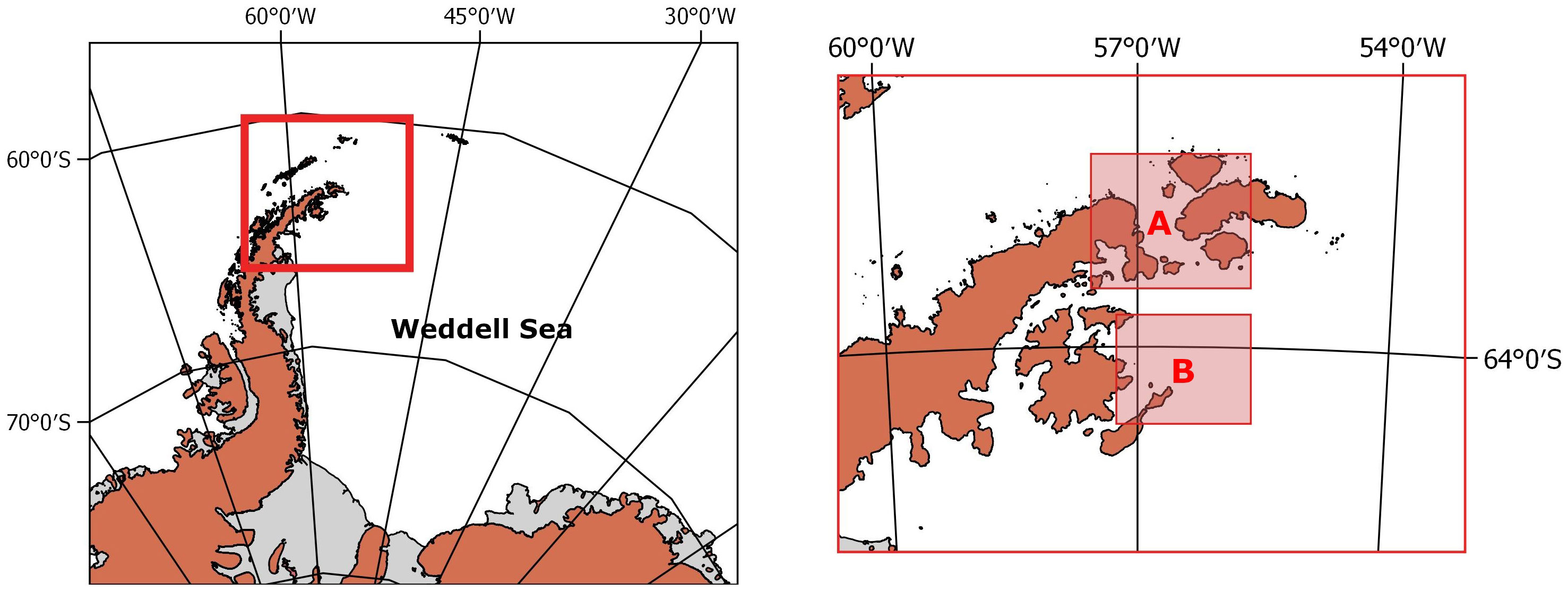
Figure 1 Study area in the north of the Antarctic peninsula (left) and detailed representation (right), showing the (A) Antarctic Sound and (B) Marambio Island and Erebus and Terror Gulf.

There were 25 images in the X-, C-, and L-bands that were analyzed corresponding to the COSMO-SkyMed, Sentinel-1, and SAOCOM satellites (Table 1). The center frequency in which the satellites operate is 9.6 GHz, 5.405 GHz, and 1.275 GHz, respectively. The images were acquired between May and September 2020. Sentinel-1 images were downloaded from the Copernicus Open Access Hub from the European Space Agency (ESA) https://scihub.copernicus.eu/dhus/. SAOCOM images were requested by the SAOCOM catalog from the Comisión Nacional de Actividades Espaciales (CONAE) https://catalog.saocom.conae.gov.ar/catalog/, and the COSMO-SkyMed images were acquired by the Agenzia Spaziale Italiana (ASI) and provided to the SHN by CONAE. The level of processing of the SAR images was in High-Resolution Ground Range Detected for Sentinel-1, Detected Image for SAOCOM, and Single-look Complex Slant for COSMO-SkyMed. For the intercomparison analysis, the dataset was divided into five groups based on an acceptable time gap between acquisitions concerning the ice regimes under study (Table 1). The use of the different groups is detailed in the next subsections.

TABLE 1

Table 1 Description of SAR image acquisitions.

The SAR images were processed using the Python Snappy module of ESA’s Sentinel Application Platform (SNAP) version 8 http://step.esa.int. Orbit correction was applied to Sentinel-1 data, and then Sentinel-1 and COSMO-SkyMed images were radiometrically calibrated to sigma naught. The exception with SAOCOM in the calibration step was because the images were obtained in Detected Image Level-1B (data projected to ground range, radiometrically calibrated, and georeferenced). Multi-looking was applied to all the images, and looks in range and azimuth were calculated using the higher range and azimuth spacing of the dataset. Subsequently, an ellipsoid correction was applied and the final projection used was the Antarctic Polar Stereographic (EPSG: 3031). To afford a comparable dataset in space resolution for the intercomparison, each image was resampled to a square pixel, the final pixel size corresponded to the largest of all the images (58.4 meters). At last, the backscatter coefficient values were converted into decibels (dB).

Meteorological data provided by the Argentine Meteorological Service (Servicio Meteorológico Nacional SMN) was used to validate the sea ice conditions. The observations were acquired from three Antarctic stations: Esperanza station (63°23′50″S 56°59′54″W) situated in the Antarctic Sound, Marambio station (64°14′50.6″S 56°37′39.3″W) in Marambio Island, and Carlini station (62°14′27.4″S 58°40′01.1″W) located in the north of the Peninsula. These stations provided measurements of air temperature, wind speed, wind direction, and precipitation (liquid or solid state) every 3 h in order to accredit the synoptic atmospheric situation.

2.2 Icebergs

The SAR response to the density of icebergs in a given area was analyzed in different SAR frequencies. All the SAR images of groups 1, 4, and 5 were used (Table 1). Particularly from group 2, the Sentinel-1 and SAOCOM images were selected, and for group 3, only the Sentinel-1 ones. The icebergs were counted in polygons of 1 km² in a fast first-year ice using the Sentinel-2 image of the 30th August 2020 near the Marambio station as a reference (Figure 2). The polygons were distributed in the fast ice covering a wide range of iceberg density, from 0 to 48 in the highest-density areas. The Sentinel-2 image, downloaded from the Copernicus Open Access Hub from the ESA, was the only optical image available in the area of high resolution and cloud-free for the period of study. Since the icebergs were trapped in fast sea ice and part of them are in a grounded area, corroborated by the SHN in the Argentine Antarctic Summer Campaign 2019-2020, the Sentinel-2 optical image was considered as a reliable source of validation.

FIGURE 2

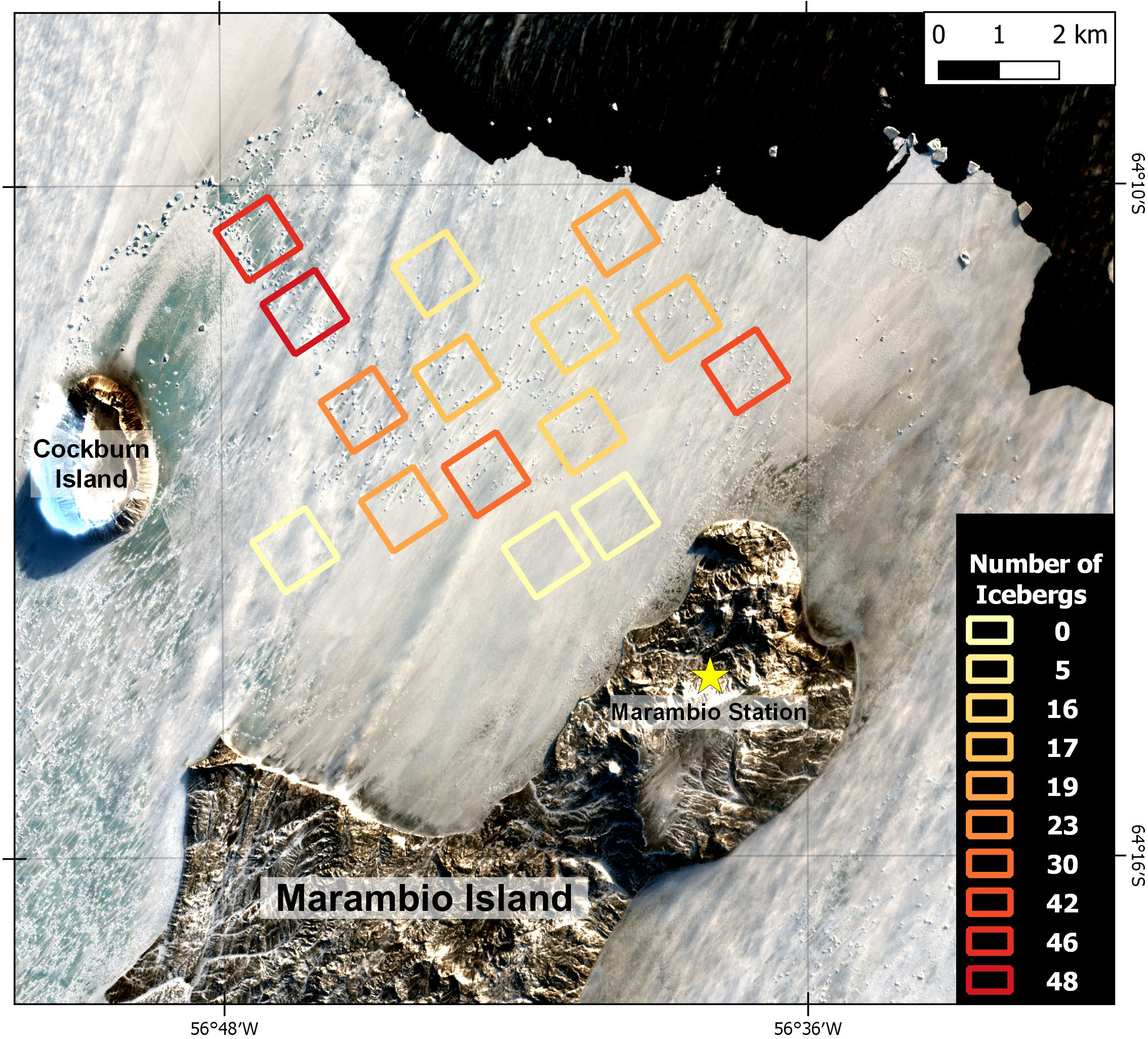
Figure 2 Iceberg sampled in the fast ice near the Marambio station. Sentinel-2 MSI 30th August 2020, bands 4-3-2. Copernicus Sentinel data 2020.

The mean and standard deviation values of the X-, C-, and L-band backscattering coefficients for HH and HV polarization were extracted from the polygons. Explanatory analysis was performed to examined the correlation among the data using the Pearson’s correlation coefficient (Equation 1).

$\begin{array}{ll}r =\frac{\sum \left((x-\overline{x})(y-\overline{y})\right)}{\surd (\sum {(x-\overline{x})}^2\ast \sum {(y-\overline{y})}^2)}& (1)\end{array}$

where r represents the Pearson correlation coefficient, x and y are the number of icebergs and the backscatter coefficient in each polygon, $\overline{\text{x}}$ is the mean of the x-values, and $\overline{\text{y}}$ is the mean of the y- values. The standard deviations of the x-values and y-values are represented in the denominator of the equation. The influence of the incidence angle in the samples was also extracted and examined. In every SAR frequency, to each SAR acquisition, a linear least-square regression model was applied to obtain the relationship between the number of icebergs and the mean backscatter values (Equation 2).

$\begin{array}{ll}\text{Y }= b_0 + b_1\text{X}& (2)\end{array}$

where Y is the dependent variable to predict, represented here as the backscatter coefficient, b₀ and b₁ are the intercept and the slope of the regression line, and X is the independent variable representing the number of icebergs per 1 km².

2.3 Fast ice features

In view of what was seen in SHN IE-2020, where spatial patterns were recognized in the different SAR frequencies, the fast ice’s features were studied at each sensor to quantify this variability. First, the hole fast ice area was jointly analyzed considering all the sea ice features together in the platform without differentiation ice characteristics. Second, the presence of snow on the fast ice and its differences observed in the SAR images were analyzed.

The analysis of the hole fast sea ice around Marambio Island was analyzed using all the SAR images of groups 1, 4, and 5 (Table 1). Specifically, from group 2 the Sentinel-1 and SAOCOM images were selected, and for group 3, only the Sentinel-1 ones. The fast ice was delineated to its minimum extent covering all the dates present in the images mentioned. For delineating the polygon, photointerpretation of the SAR images was performed and optical imagery was used as validation when available from the Sentinel-2 or MODIS (Moderate Resolution Imaging Spectroradiometer). Sentinel-2 was obtained as mentioned in Section 2.2, and MODIS was consulted on NASA (National Aeronautics and Space Administration) Worldview application https://worldview.earthdata.nasa.gov, part of NASA’s Earth Observing System Data and Information System (EOSDIS). After the delimitation of the fast ice area, values were extracted to all the images and the frequency distribution of the data was analyzed.

The analysis of the presence of the snow cover on the fast ice was done comparing the backscatter of bare and snow-covered first-year ice near Cockburn Island in the Erebus and Terror Gulf. From the Sentinel-2 image of the 30th August 2020, snow-covered and bare sea ice were identified and circular samples were collected with a 50 m radius (Figure 3). Mean values were calculated to each sample; afterward, to each SAR image, mean values for the snow-covered areas and bare ice were evaluated, and the difference of the same were performed following Equation 3:

FIGURE 3

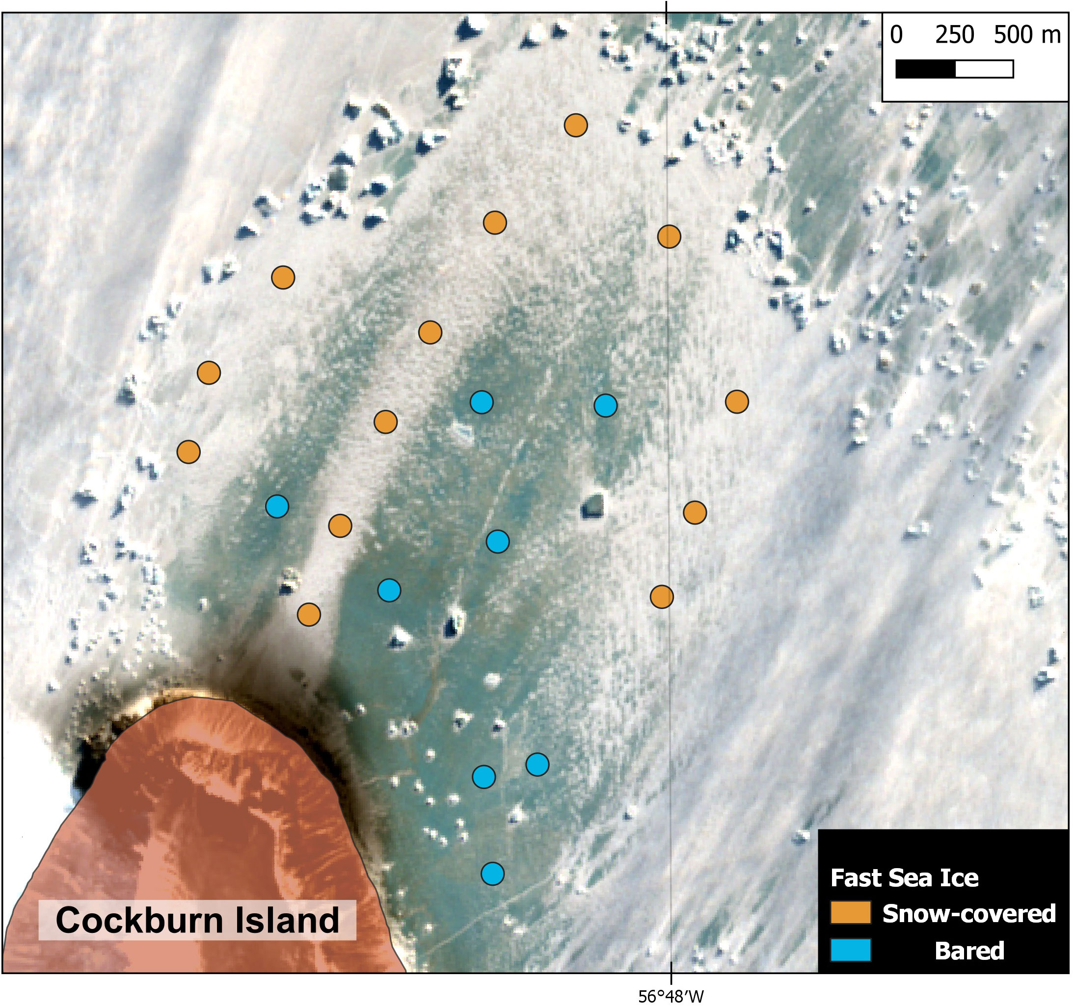
Figure 3 Snow-covered and bare samples on the fast ice north of Cockburn Island. Sentinel-2 MSI 30th August 2020, bands 4-3-2. Copernicus Sentinel data 2020.

$\begin{array}{ll}\text{Dif}{\text{f}}_{\text{s}-\text{b}}={10}^{*}{\text{log}}_{10}({\sigma }_{\text{s}}-{\sigma }_{\text{b}})& (3)\end{array}$

where Diff_s-b is the difference between the snow-covered and bare ice areas as the difference of the power per unit area of the snow-covered ice σ_s and the power per unit area of the bare ice σ_b, converted in decibels. The SAR images used to calculate this difference were from the 21st August to 13th September corresponding to groups 4 and 5 (Table 1). Meteorological data were used to validate the use of optical imagery as ground truth. Meteorological observations were taken from the Marambio station with 51 days of accumulated days of precipitation registered, showing 102.1 mm of snow recorded since the formation of the fast ice. Maximum and minimum temperatures were below 0°C with a prevailing wind direction from the south to southwest, accumulating 48% of the daily observations in that direction. Patterns in the snow cover to the north of Cockburn Island were visualized in the Sentinel-2 image, confirming the recorded observations (Figure 3).

2.4 Belts and strips

Strips and belts present in the Antarctic Sound were analyzed, and the images used correspond to groups 2 and 3. In order to compare backscatter values for sea and water around, strip and water samples were selected at similar incidence angles (Figure 4). The samples were determined visually using HH and HV polarization of each band. Boxplots were plotted for each pair of samples (strips and water) and for each band so as to facilitate the comparison between samples (comparison of backscatter values and standard deviation). To ensure a detailed analysis of the backscatter values of strips and water, the wind speed and direction data were taken from the Esperanza station, corresponding to the dates of image acquisition (Table 1).

FIGURE 4

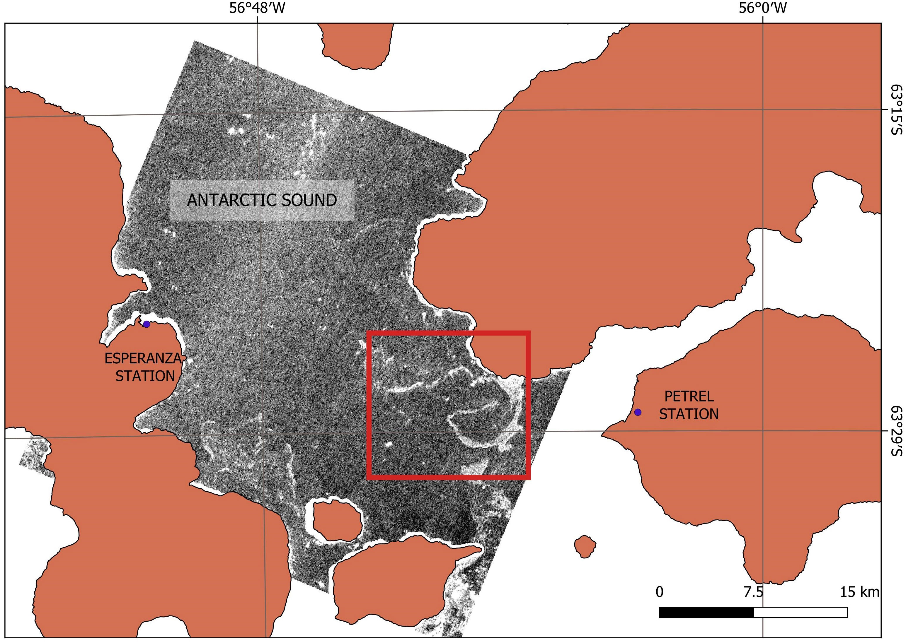
Figure 4 The study area for the analysis of strips and belts. The red box shows the area where the samples of ice and water were taken. The satellite image correspond to the SAOCOM image of 15th May 2020. SAOCOM® Product – ©CONAE – 2020. All Rights Reserved.

3 Results and discussion

3.1 Icebergs

The Pearson correlation coefficients were low for all the SAR frequencies and above zero, determining a positive weak relation between the number of icebergs and the backscattering coefficients in the X-, C-, and L-bands for each polarization (Figure 5). The C- and L-bands showed a wider value range in the backscattering coefficient since more image acquisition was analyzed in those frequencies.

FIGURE 5

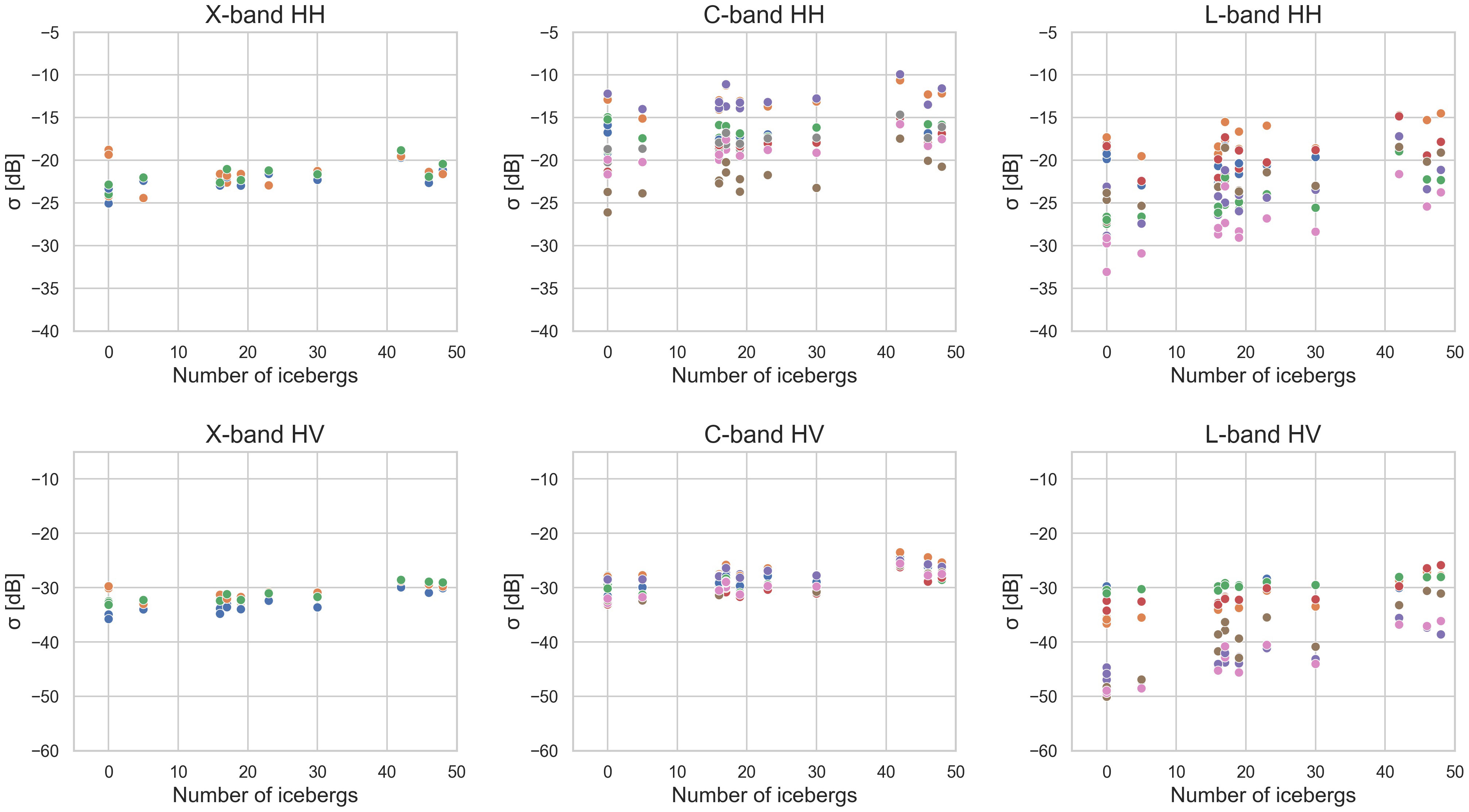
Figure 5 X-, C-, and L-band backscattering coefficients in dB for HH (top) and HV (bottom) polarization vs. different numbers of icebergs in 1 km². Different colors identify different SAR acquisitions.

To quantify the nature of the relationship between the number of icebergs per km² and the backscatter coefficient in different SAR frequencies, linear regression models were performed. The coefficient of determination of the models (R²) was low for most of the acquisition in HH polarization in all the frequencies and with p-values that were only significant to 0.05 for two images of three in the X-band, five images of eight in the C-band, and six images of seven in the L-band (Table 2). HV polarization showed higher R² values than HH polarization with only one image in the X-band, three in the C-band, and one in the L-band with lower values than 0.7; all p-values were significant (Table 2). The slope for the linear model was higher in the L-band than in the X- and C-bands.

TABLE 2

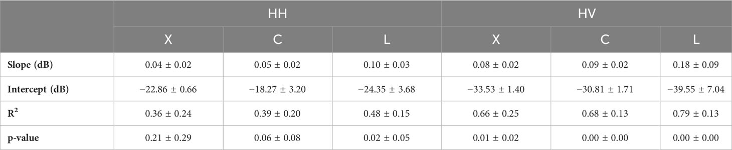
Table 2 Mean and standard deviation for each linear regression per image acquisition in each SAR frequency.

The incidence angle where the polygons were located was contrasted with its response in the HH and HV channels. The difference in the backscatter coefficient for areas with low vs. high amounts of icebergs increases with the incidence angle in both polarizations (Figure 6). Because the availability in C- and L-band imagery was larger than the X-band, a broader range of incidence angles was presented in the dataset for those frequencies, making the analysis of the X-band inconclusive for evaluating the effect of the incidence angle. The L-band showed a large interval between the minimum and maximum of backscatter values in HV polarization. The standard deviation range obtained for the backscattering coefficient in HH polarization was 1.24–1.6 dB for the X-band, 1.14–2.07 dB for the C-band, and 1.75–3.03 dB for the L-band; meanwhile, for HV, polarization was 1.33–1.78 dB for the X-band, 1.13–2.08 dB for the C-band, and 2.5–6.18 dB for the L-band.

FIGURE 6

Figure 6 X-, C-, and L-band backscattering coefficients in dB for HH and HV polarization vs. incidence angle in degrees. Each color represents one SAR image, and the saturation corresponds to the increase in the number of icebergs sampled.

The higher variability of the L-band in HV polarization evidences greater sensitivity of the L-band to the presence of icebergs than the C- and X-bands, with the exception of one TOPSAR Narrow image, in which thermal noise was observed on one of the sub-swaths, the position in which the samples were taken. Additional analysis of the TOPSAR Narrow mode is required to ameliorate the effect or reduce the thermal noise in the sub-swath.

3.2 Fast ice features

The fast ice around Marambio Island contains multiyear ice, north of Marambio station, which was grounded prior to freezing (Figure 7). Of all the frequencies, the L-band was the one that showed a closer representation of HH polarization to the optical images, accurately following the fast sea ice composition and evolution, highlighting the variety of features in the ice (Figure 7).

FIGURE 7

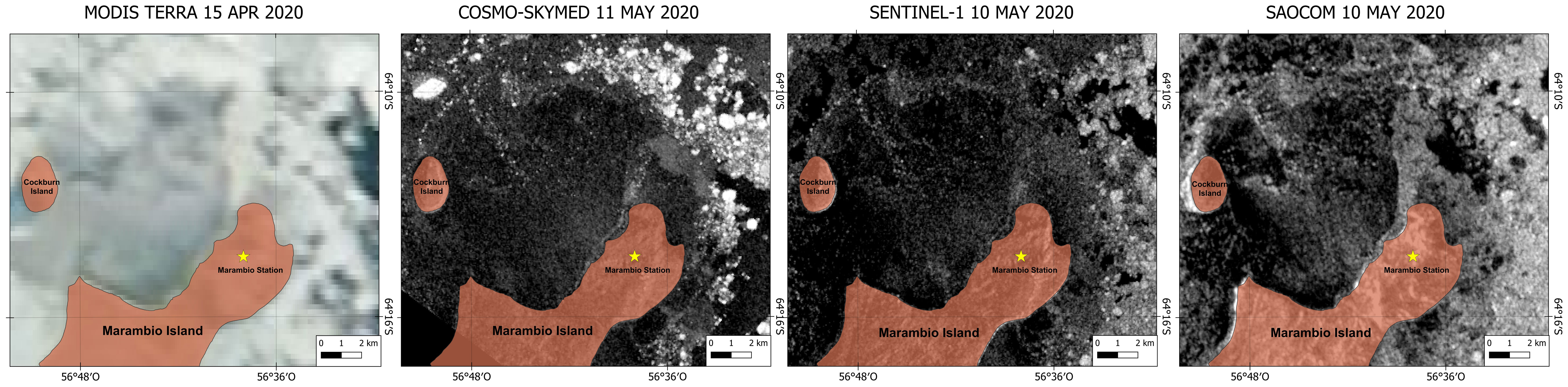
Figure 7 Fast ice’s formation near Marambio Island on MODIS Terra. The same area in the X-, C-, and L-band images, backscattered in dB for HH polarization. Copernicus Sentinel data 2020. SAOCOM® Product – © CONAE – 2020, All Rights Reserved. COSMO-SkyMed Product – ^© ASI 2020 processed under license from ASI – Agenzia Spaziale Italiana, All Rights Reserved, and distributed by CONAE.

The distribution of the backscattering response in dB was analyzed for each intercomparison group in the fast ice area (Figure 8). Conclusions about the range of the backscattering coefficient cannot be done because of the wide range in the incidence angles present in the dataset. In HH polarization, the L-band from SAOCOM showed higher variability in the backscatter values as can be seen in the histograms for all the intercomparison dates (Figure 8). The standard deviation in dB obtained for HH polarization in the first group was 3.58 for the X-band, 3.58 for the C-band, and 3.61 for the L-band. For the second and third groups, it was 3.21–3.28 for the C-band and 4.48 for the L-band. Lastly, in the fourth group, the standard deviation was 3.29–3.47 for the C-band and 4.31–5.6 for the L-band, and for the fifth group it was 3.93–4.13 for the X-band and 3.18–4.36 and 4.1–5.26 for the L-band.

FIGURE 8

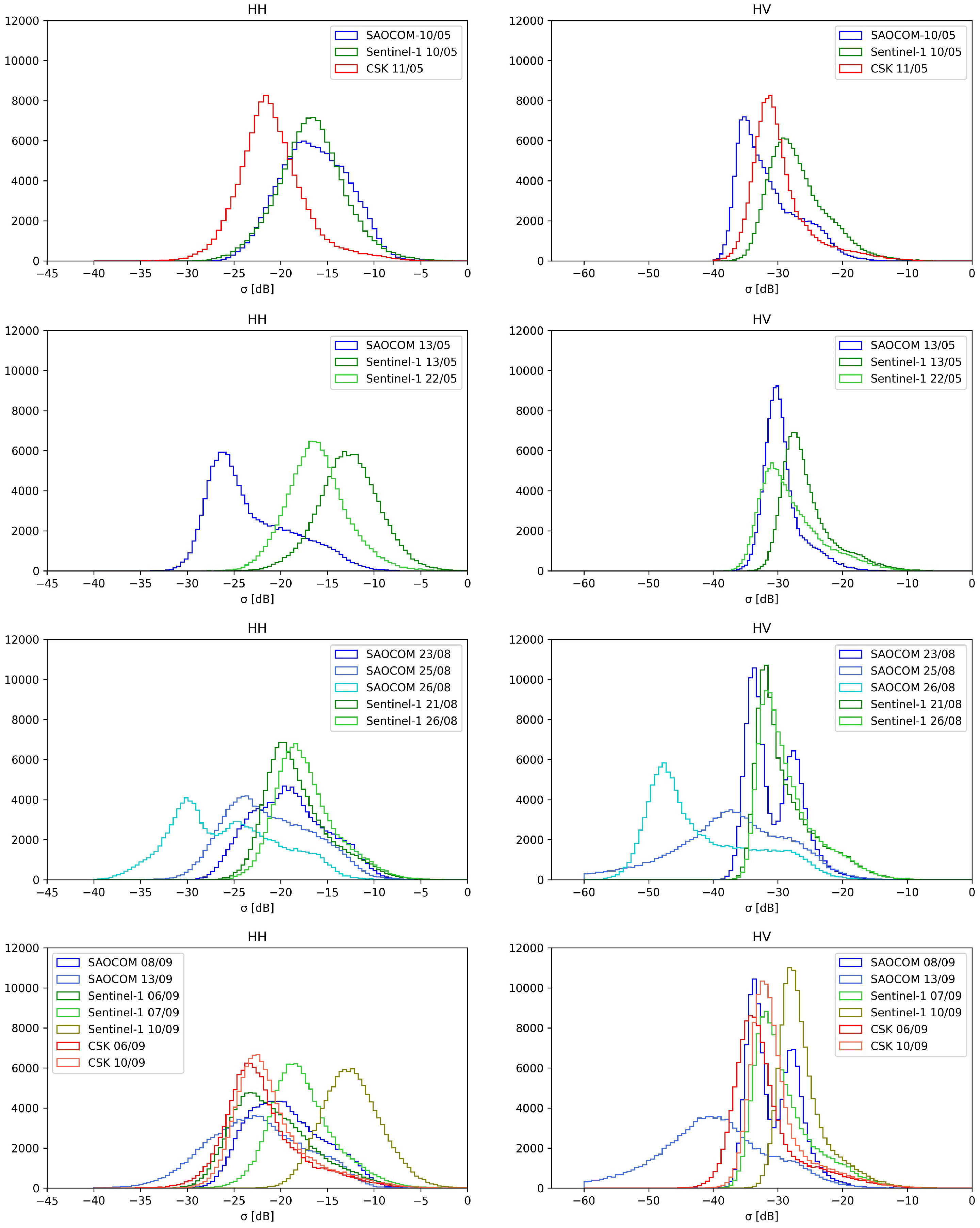
Figure 8 Histogram distribution of SAR images in the X-, C-, and L-bands for (from top to bottom) groups 1, 2 and 3, 4, and 5. HH polarization is represented to the left and HV to the right.

HV polarization presented less variability in the data distribution than HH polarization, with similar curves for each frequency, with the exception of SAOCOM images from the fourth and fifth intercomparison groups, corresponding to two images with incidence angles upper 33°, Stripmap and TOPSAR Narrow mode, and a TOPSAR Wide image with a nominal incidence angle of 25.5° in the fast ice area. SAOCOM images from 23rd August and 8th September showed a bimodal distribution that was caused by the thermal noise in one of the sub-swaths of the TOPSAR Narrow Mode, as it was explained in the previous subsection.

For the analysis of the snow presence on the fast ice, the SAR frequency did not show a distinction between the backscatter coefficient of bare and snow-covered first-year ice, and the variability observed in the results was attributed to differences in the SAR parameters. However, the polarization channel showed an impact on the snow detection with all the differences between the bare and snow-covered positive in HH polarization, 75% of the images above 2 dB of difference (Figure 9). In HV polarization, the differences were lower, with three images from SAOCOM and from COSMO-SkyMed below zero (Figure 9). Patterns in the variability presented in the results considering the SAR frequency, incidence angle, resolution of the image, direction of the antenna in relation to the area sampled, and weather conditions were studied; nonetheless, causes cannot be attributed because the differences in the dataset and more images need to be included to reach conclusions.

FIGURE 9

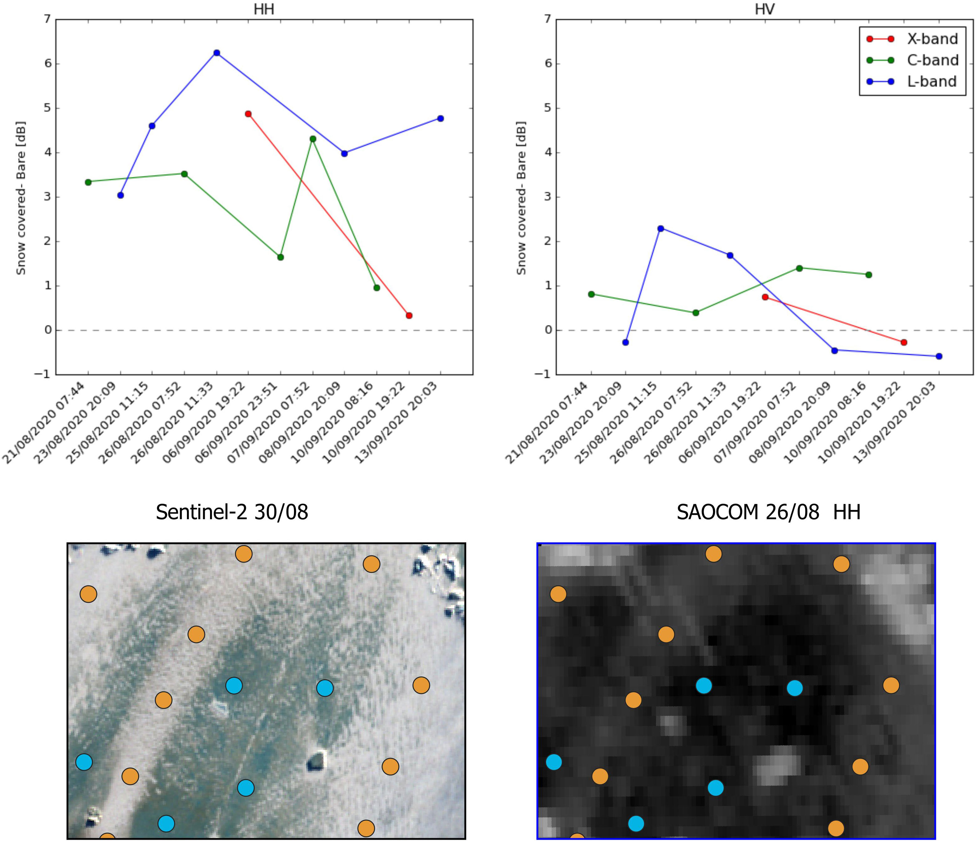
Figure 9 Difference between snow-covered and bare samples mean on the fast ice north of Cockburn Island for HH and HV polarization in the X-, C-, and L-bands. Copernicus Sentinel data 2020. SAOCOM® Product – © CONAE – 2020, All Rights Reserved.

In HH polarization, SAOCOM showed an increase in the bare and snow-covered difference between 23rd and 26th August, a period in which snowfalls occurred, and a similarity in the bare and snow-covered difference from 8th to 13th September, a date interval without precipitation (Figure 9). Further research needs to be done on the L-band, since the results revealed a sensitivity to snow precipitation but the dataset is not large enough to conclude.

3.3 Belts and strips

Figure 10 shows the images analyzed on the Antarctic Sound; the backscatter values of strips and water were compared, and the result is shown in Figure 11.

FIGURE 10

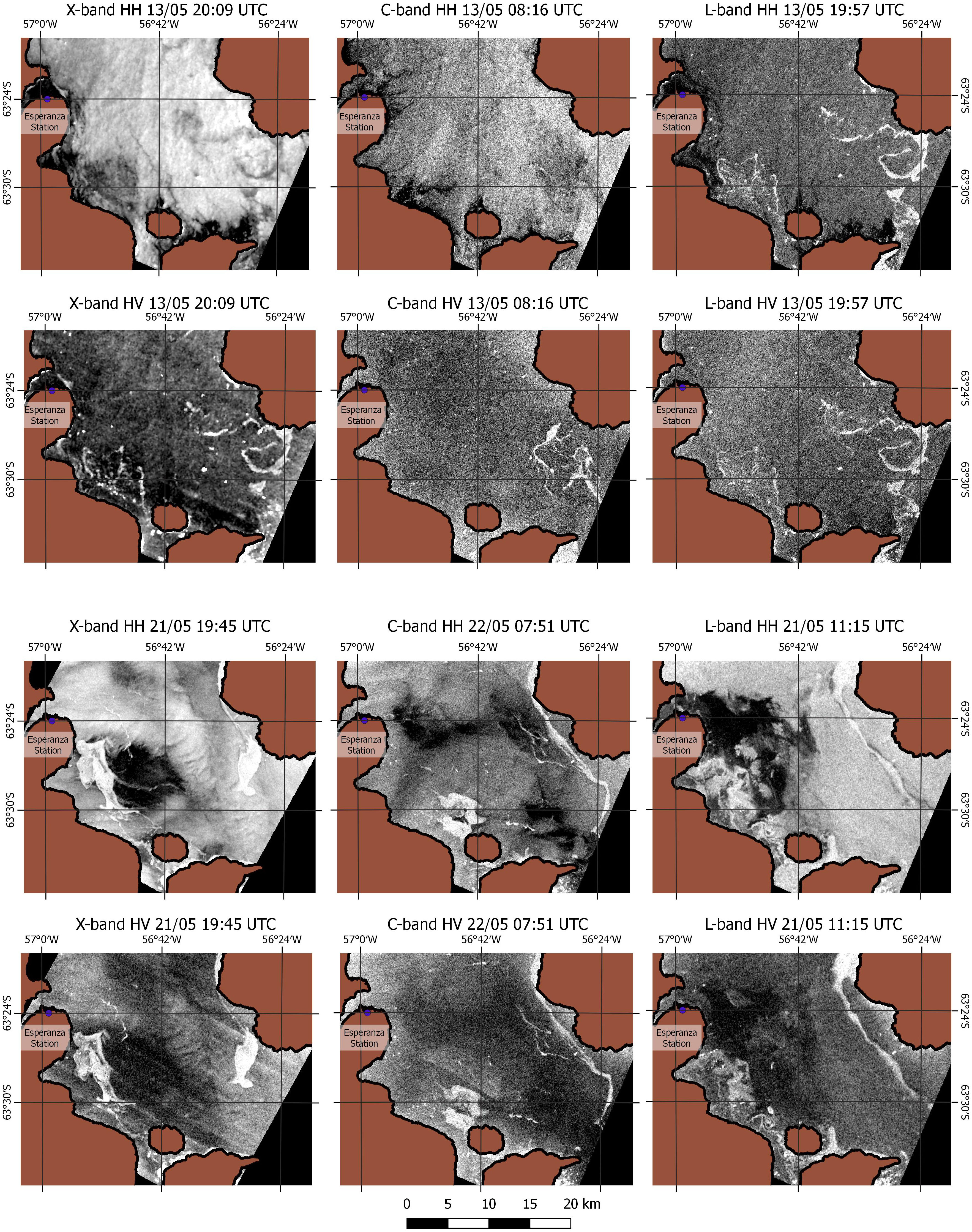
Figure 10 X-, C-, and L-band backscattering coefficients in dB for HH and HV polarization. Copernicus Sentinel data 2020. SAOCOM® Product – © CONAE – 2020, All Rights Reserved. COSMO-SkyMed Product – © ASI 2020 processed under license from ASI – Agenzia Spaziale Italiana, All Rights Reserved, and distributed by CONAE.

FIGURE 11

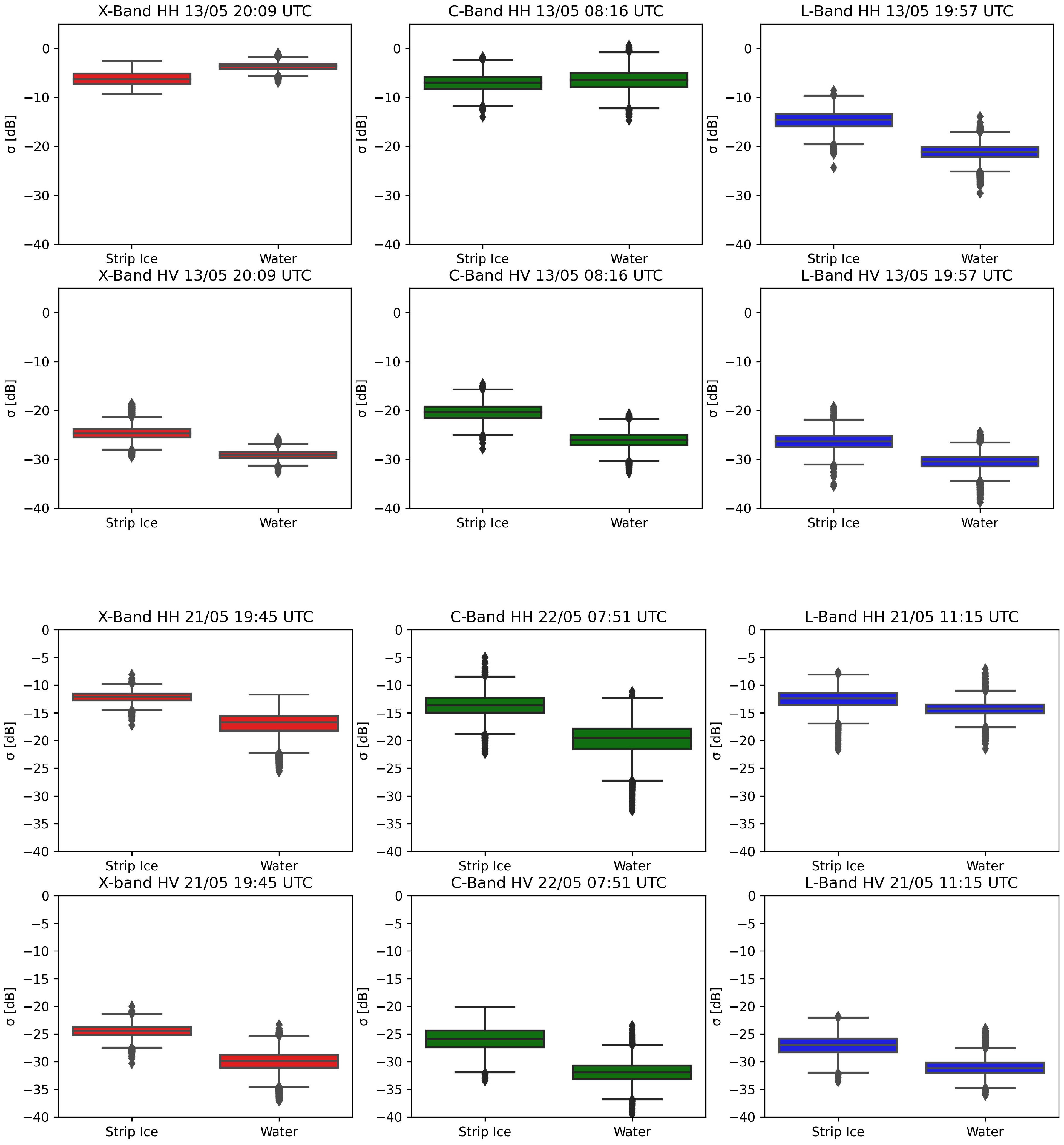
Figure 11 Boxplots of backscatter at X-, C-, and L-bands for open water and strips.

For most of the analyzed cases, the HV polarization showed an advantage for strip detection with respect to HH polarization; this result was noted in the visual and quantitative analyses (Figure 11) where the backscatter values for the water box were below the values for the strip ice box. A clear example was found in the C-band image from 13th May, where it was not possible to distinguish the presence of ice in HH (both samples had similar backscatter values), whereas in HV the presence of strips was observed. This advantage of HV polarization may be due to a higher sensitivity of HH polarization to the wind effect on the ocean surface. This result is consistent with previous studies where the water backscatter values in HV are lower than those of HH even under wind roughened conditions (Shuchman and Flett, 2003; Arkett et al., 2007).

In some cases, the sea surface presented more backscattering than sea ice like X-band image from 13th May, where sea ice had dark tones and the backscatter values for the strip ice box were below the values for the water box. This could be a result of a greater roughness of the sea surface with respect to the ice surface. The dark tones for sea ice in SAR images must be taken into account by the ice analysts when the presence of sea ice is analyzed. This effect was reported previously in the ice edge zone by Onstott and Shuchman (2004) and by Arkett et al. (2007).

In the inter-band analysis, it was observed that in the case of group 2, in the C-band image with HH polarization, it was not possible to identify and differentiate the sea ice from the water around it, unlike the X- and C-band images with HH polarization. According to the wind measurements reported at the closest meteorological station to the study area, there was a decrease of approximately 60% in the intensity of the wind between the acquisition of the C-band and X- and L-band images (Figure 12). An increase in the intensity of the wind over the sea produces a growth in the roughness of the sea surface, in turn increasing the backscattering of the surface. This results in sea surface roughness, and its response could be limiting the detection of sea ice at HH polarization.

FIGURE 12

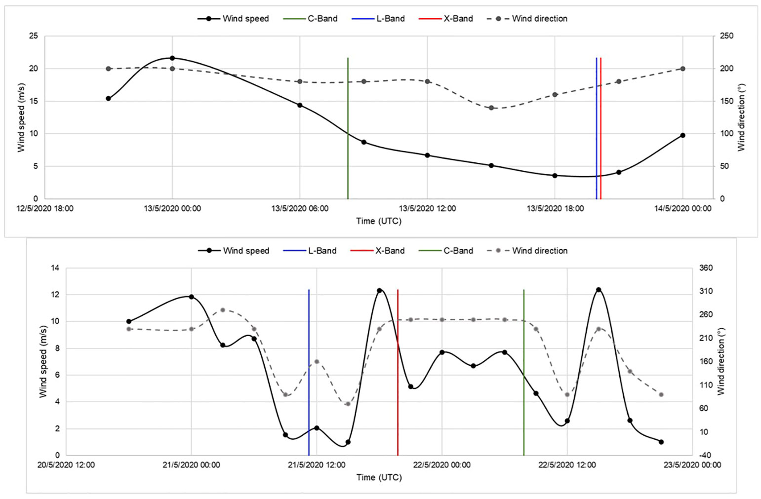
Figure 12 Evolution for wind parameters in Esperanza station during May.

The X- and L-band images of group 2 were acquired within 12 min apart, and no evidence was found that the meteorological conditions were significantly modified in that time period. However, a better distinction was noted for L-band both visually and in the boxplots, with a greater difference between samples. The differences between X- and L-band could be due to the intrinsic characteristics of each band. This would represent an advantage for the L-band in distinguishing sea ice strips from water, being L-band less sensitive to the wind or the sea state compared with X-band as Dierking et al., 2022 indicated in their study. However, differences in the incidence angles of each acquisition make it difficult to determine a conclusive cause.

For the acquisition dates of group 3, no significant variations in wind intensity (Figure 12) or a particular pattern in wind behavior were found. In all the bands, it was possible to identify and differentiate the water from the strips. The differences between bands may be due to the characteristics of each image acquisition (space resolution and incidence angle).

4 Conclusion

This paper presents the quantitative results obtained from a detailed previous Intercomparison Experiment carried out in 2020 (IE-2020) by the Argentine Naval Hydrographic Service using the X-, C-, and L-bands from the COSMO-SkyMed, Sentinel-1, and SAOCOM, respectively. The analysis was performed following typical sea ice and iceberg operational conditions: (i) icebergs, (ii) fast ice features, and (iii) belts and strips.

The results found with the HV polarization of SAOCOM suggested the L-band as a convenient frequency for the detection of areas with a high density of icebergs surrounded by first-year ice. The number of icebergs showed positive but weak correlations with the backscatter coefficient in HH polarization for all the sensors; however, significant results were obtained in HV polarization, even under different SAR parameters such as image acquisition and different incidence angles. The linear regressions presented showed the L-band as the frequency with a higher slope and coefficient of determination, being significant in HV polarization, with good results even under spatial resolutions of around 100 m for the TOPSAR Wide Quad polarization mode.

As it was seen from visual interpretation in the IE-2020, the analysis of the fast first-year ice near Marambio Island revealed a higher sensitivity to the surface features of the L-band, consistent with the evolution and composition of the fast ice. No influence in the backscattering coefficient was observed on the different SAR frequencies in relation to the snow layer on the first-year ice; nevertheless, polarization was important in its detections, with measurable differences in the HH channel.

The identification of strips and belts in seawater depended on the sea state and wind conditions in the area. The HV polarization represented an advantage in the identification in relation to HH polarization because of the lower sensitivity to the surface water roughness. The L-band showed to be less sensitive to the roughness of the sea surface; however, further analysis is needed to determine a benefit in the detection of strips with the L-band. Additionally, future research has to be done to incorporate in the SAOCOM image processing workflow the reduction in sub-swath thermal noise, as was seen in two TOPSAR Narrow images from our dataset.

In addition to the limitation in part of the results found, the dataset used in this intercomparison showed the typical operational situation in the Ice Services, where any SAR acquisition is valuable to approach the last most updated condition of the sea ice and icebergs. Further research still needs to be developed in view of incorporating the broad variability in SAR parameters, such as diversity in acquisition modes, resolution, polarization, incidence angle, different environmental conditions, and season of the year to generate useful outcomes for decision-making.

Data availability statement

The raw data supporting the conclusions of this article will be made available by the authors, without undue reservation.

Author contributions

CS: Writing – original draft, Writing – review & editing. LG: Writing – original draft, Writing – review & editing. JA: Writing – original draft, Writing – review & editing.

Funding

We would like to thank the World Meteorological Organization (WMO) for all the support that has been provided to the Argentine Hydrographic Service over the years, and for the financial support that has made this publication possible and open to the scientific community and operational users.

Acknowledgments

We would like to thank the Comisión Nacional de Actividades Espaciales (CONAE) for the provision of the SAOCOM® Product – © CONAE – 2020 All Rights Reserved, and to all personnel that helped us during the process of incorporating the SAOCOM satellite in our Ice Service, especially Laura Frulla, Mario Camuyrano, and Marcela Jauregui, and the great support from the technical support team with the SAOCOM catalog. We acknowledge Copernicus Sentinel data 2020, and COSMO-SkyMed Product – © ASI 2020 processed under license from ASI – Agenzia Spaziale Italiana, All Rights Reserved, distributed by CONAE. We acknowledge the use of imagery from the Worldview Snapshots application (https://wvs.earthdata.nasa.gov), part of the Earth Observing System Data and Information System (EOSDIS). Finally, we are grateful to the reviewers whose comments contributed to the readability and clarity of this paper.

Conflict of interest

The authors declare that the research was conducted in the absence of any commercial or financial relationships that could be construed as a potential conflict of interest.

Publisher’s note

All claims expressed in this article are solely those of the authors and do not necessarily represent those of their affiliated organizations, or those of the publisher, the editors and the reviewers. Any product that may be evaluated in this article, or claim that may be made by its manufacturer, is not guaranteed or endorsed by the publisher.

References

Anconitano G., Acuña M. A., Guerriero L., Pierdicca N. (2022). “Analysis of multi-frequency SAR data for evaluating their sensitivity to soil moisture over an agricultural area in Argentina,” in IGARSS 2022 - 2022 IEEE International Geoscience and Remote Sensing Symposium, Kuala Lumpur, Malaysia, pp. 5716–5719. doi: 10.1109/IGARSS46834.2022.9884232

CrossRef Full Text | Google Scholar

Arkett M., Flett D. G., Abreu R. D. (2007). “B-band multiple polarization SAR for ice monitoring - What can it do for the Canadian ice Service,” in Proceedings of the Envisat Symposium 2007 Montreux, Switzerland (ESA SP-636, July 2007). pp. 23–27.

Google Scholar

Arkett M., Flett D., Abreu R. D., Clemente-Colon P., Woods J., Melchior B. (2008). “Evaluating ALOS-PALSAR for ice monitoring—What can L-band do for the North American ice service?” in IGARSS 2008 - 2008 IEEE International Geoscience and Remote Sensing Symposium, Boston, MA, USA, pp. V-188–V-191. doi: 10.1109/IGARSS.2008.4780059

CrossRef Full Text | Google Scholar

Azcueta M., Gonzalez J. P. C., Zajc T., Ferreyra J., Thibeault M. (2022). "External calibration results of the SAOCOM-1A commissioning phase,". IEEE Trans. Geosci. Remote Sens. 60, 1–8. doi: 10.1109/TGRS.2021.3075369. 2022, Art no. 5207308.

CrossRef Full Text | Google Scholar

Blomberg E., Ferro-Famil L., Soja M. J., Ulander L. M. H., Tebaldini S. (2018). "Forest biomass retrieval from L-band SAR using tomographic ground backscatter removal,". IEEE Geosci. Remote Sens. Lett. 15 (7), 1030–1034. doi: 10.1109/LGRS.2018.2819884

CrossRef Full Text | Google Scholar

Casey J. A., Howell S. E. L., Tivy A., Haas C. (2016). Separability of sea ice types from wide swath C- and L-band synthetic aperture radar imagery acquired during the melt season. Remote Sens. Environ. 174, 314–328. doi: 10.1016/j.rse.2015.12.021

CrossRef Full Text | Google Scholar

De Luca C., Roa Y., Bonano M., Casu F., Manunta M., Manzo M., et al. (2022). “On the first results of the DInSAR-3M project: A focus on the interferometric exploitation of saocom SAR images,” in IGARSS 2022 - 2022 IEEE International Geoscience and Remote Sensing Symposium, Kuala Lumpur, Malaysia, pp. 4502–4505. doi: 10.1109/IGARSS46834.2022.9884715

CrossRef Full Text | Google Scholar

Dierking W. (2013). Sea ice monitoring by synthetic aperture radar. Oceanography 26 (2), 100–111. doi: 10.5670/oceanog.2013.33

CrossRef Full Text | Google Scholar

Dierking W., Busche T. (2006). Sea ice monitoring by L-band SAR: an assessment based on literature and comparisons of JERS-1 and ERS-1 imagery. IEEE Trans. Geosci. Remote Sens. 44 (4), 957–970. doi: 10.1109/TGRS.2005.861745

CrossRef Full Text | Google Scholar

Dierking W. (2021). “Synergistic use of L- and C-band SAR satellites for sea ice monitoring,” in 2021 IEEE International Geoscience and Remote Sensing Symposium IGARSS, Brussels, Belgium, pp. 877–880. doi: 10.1109/IGARSS47720.2021.9554359

CrossRef Full Text | Google Scholar

Dierking W., Iannini L., Davidson M. (2022). “Joint use of L-and C-band spaceborne SAR data for sea ICE monitoring,” in IGARSS 2022 - 2022 IEEE International Geoscience and Remote Sensing Symposium, Kuala Lumpur, Malaysia, pp. 4711–4712. doi: 10.1109/IGARSS46834.2022.9884133

CrossRef Full Text | Google Scholar

Drinkwater M. R., Kwok R., Winebrenner D. P., Rignot E. (1991). Multi-frequency polarimetric synthetic aperture radar observations of sea ice. J. Geophys. Res. 96 (C11), 20,679–20,698. doi: 10.1029/91JC01915

CrossRef Full Text | Google Scholar

Ferreyra J., Solorza R., Teverovsky S., Soldano A. (2021). “Estimación de dirección y velocidad superficial en glaciares de la Patagonia Austral utilizando datos de la constelación SIASGE.” in 2021 XI Congreso Argentino Tecnología Espacial, pp. 7–9.

Google Scholar

Flett D., De Abreu R., Arkett M., Gauthier M.-F. (2008). “Initial evaluation of Radarsat-2 for operational sea ice monitoring,” in IGARSS 2008 - 2008 IEEE International Geoscience and Remote Sensing Symposium, Boston, MA, USA, pp. I-9–I-12. doi: 10.1109/IGARSS.2008.4778779

CrossRef Full Text | Google Scholar

Han H., Kim J. I., Hyun C. U., Kim S. H., Park J. W., Kwon Y. J., et al. (2020). Surface roughness signatures of summer arctic snow-covered sea ice in X-band dual-polarimetric SAR. GIScience Remote Sens. 57 5, 650–669. doi: 10.1080/15481603.2020.1767857

CrossRef Full Text | Google Scholar

Johansson A. M., Brekke C., Spreen G., King J. A. (2018). X-, C-, and L-band SAR signatures of newly formed sea ice in Arctic leads during winter and spring. Remote Sens. Environ. 204, 162–180. doi: 10.1016/j.rse.2017.10.032

CrossRef Full Text | Google Scholar

Johansson A. M., King J. A., Doulgeris A. P., Gerland S., Singha S., Spreen G., et al. (2017). Combined observations of Arctic sea ice with near-coincident colocated X-band, C-band, and L-band SAR satellite remote sensing and helicopter-borne measurements. J. Geophysical Research: Oceans 122 (1), 669–691. doi: 10.1002/2016JC012273

CrossRef Full Text | Google Scholar

Kwok R., Cunningham C. F., Nghiem. S. V. (2003). A study of the onset of melt over the Arctic Ocean in RADARSAT synthetic aperture radar data. J. Geophysical Res. 108, 3363. doi: 10.1029/2002JC001363

CrossRef Full Text | Google Scholar

Lyu H., Huang W., Mahdianpari M. (2022). “A meta-analysis of sea ice monitoring using spaceborne polarimetric SAR: advances in the last decade,” in IEEE Journal of Selected Topics in Applied Earth Observations and Remote Sensing, 15, 6158–6179. doi: 10.1109/JSTARS.2022.3194324

CrossRef Full Text | Google Scholar

MaChado F., Solorza R. (2020). “Feasibility of the inversion of electromagnetic models to estimate soil salinity using SAOCOM data,” in 2020 IEEE Congreso Bienal de Argentina (ARGENCON), Resistencia, Argentina, pp. 1–8. doi: 10.1109/ARGENCON49523.2020.9505383

CrossRef Full Text | Google Scholar

Maillard P., Clausi D. A., Deng H. (2005). Operational map-guided classification of SAR sea ice imagery IEEE Trans. Geosci. Remote Sens. 43 (12), 2940–2951. doi: 10.1109/TGRS.2005.857897

CrossRef Full Text | Google Scholar

Matsuoka T., Uratsuka S., Satake M., Kobayashi T., Nadai A., Umehara T., et al. (2001). CRL/NASDA airborne SAR (Pi-SAR) observations of sea ice in the Sea of Okhotsk. Ann. Glaciology 33, 115–119. doi: 10.3189/172756401781818734

CrossRef Full Text | Google Scholar

Onstott R. G., Shuchman R. A. (2004). “SAR measurements of sea ice,” in Synthetic Aperture Radar:Marine User's Manual. Eds. Jackson C. R., Apel J. R. (Washington, DC: Synthetic Aperture Radar MarineUser's Manual. NOAA), 81–115.

Google Scholar

Roa Y., Rosell P., Solarte A., Euillades L., Carballo F., García S., et al. (2021). First assessment of the interferometric capabilities of SAOCOM-1A: New results over the Domuyo Volcano, Neuquén Argentina. J. South Am. Earth Sci. 106, 102882. doi: 10.1016/j.jsames.2020.102882. ISSN 0895-9811.

CrossRef Full Text | Google Scholar

Salvó C. S., Gómez Saez L., Scardilli A., Salgado H. (2022). “Incorporación del Sar Saocom para el monitoreo operativo del hielo marino y témpanos,” in Centro de Estudios de Prospectiva Tecnológica Militar TEC 1000 / 1a ed. (Ciudad Autónoma de Buenos Aires: Universidad de la Defensa Nacional), 216, 173–182. Available at: https://www.fie.undef.edu.ar/ceptm/wp-content/uploads/2022/10/TEC1000-2021-Digital.pdf.

Google Scholar

Scardilli A. S., Salvó C. S., Gomez Saez L. (2022). Southern Ocean ice charts at the Argentine Naval Hydrographic Service and their impact on safety of navigation. Front. Mar. Sci. 9. doi: 10.3389/fmars.2022.971894

PubMed Abstract | CrossRef Full Text | Google Scholar

Seppi S. A., Casanova E. S., Roa Y. L. B., Euillades L., Gaute M. (2021). On the feasibility of applying orbital corrections to SAOCOM-1 data with free open source software (foss) to generate digital surface models: a case study in Argentina. Int. Arch. Photogrammetry Remote Sens. Spatial Inf. Sci. 46, 167–174. doi: 10.5194/isprs-archives-XLVI-4-W2-2021-167-2021

CrossRef Full Text | Google Scholar

Shuchman R. A., Flett D. G. (2003). “SAR measurement of sea ice parameters: sea ice session overview paper”. in Proceedings of the Second Workshop on Coastal and Marine Applications of SAR (CMASAR), 8 – 12 September 2003, Svalbard, Norway (ESA SP-565, June 2004). p. 151–160.

Google Scholar

Singha S., Johansson M., Hughes N., Hvidegaard S., Skourup H. (2018). Arctic sea ice characterization using spaceborne fully polarimetric L-, C- and X-band SAR with validation by airborne measurements. IEEE Trans. Geosci. Remote Sens. 56 (7), 3715–3734. doi: 10.1109/TGRS.2018.2809504

CrossRef Full Text | Google Scholar

Viotto S., Bookhagen B., Toyos G., Torrusio S. (2021). “Assessing ground deformation in the Central Andes (NW Argentina) with Interferometric Synthetic Aperture Radar analyses: First results of SAOCOM data and Sentinel-1 data,” in EGU General Assembly 2021, online, 19–30 Apr 2021, EGU21–12474. doi: 10.5194/egusphere-egu21-12474

CrossRef Full Text | Google Scholar

Wang Y. R., Li X. M. (2021). Arctic sea ice cover data from spaceborne synthetic aperture radar by deep learning. Earth Syst. Sci. Data 13, 2723–2742. doi: 10.5194/essd-13-2723-2021

CrossRef Full Text | Google Scholar

Zakhvatkina N. Y., Alexandrov V. Y., Johannessen O. M., Sandven S., Frolov I. Y. (2012). Classification of sea ice types in ENVISAT synthetic aperture radar images. Geosci. RemoteSensing 51 (5), 2587–2600. doi: 10.1109/TGRS.2012.2212445

CrossRef Full Text | Google Scholar