Assessing ocean ensemble drift predictions by comparison with observed oil slicks

Geophysical models are cornerstone pieces in marine forecasting of floating objects and pollution, such as marine surface oil slicks. Trajectory forecasts of oil spills inherit the uncertainties from the underlying geophysical forcing. In this work we compare the forecast capabilities of an ocean ensemble prediction system (EPS) to those from a higher resolution deterministic model on the representation of oil slick drift. As reference, we use produced water (PW) slicks detected and delineated from 41 C–band Sentinel-1A/B satellite synthetic aperture radar images between April and December, 2021. We found that the EPS provided at least equivalent member-wise results relative to simulations forced with the deterministic model. Ensemble verification through rank histograms and spread-error relationship showed that including the ocean fields is necessary to address model uncertainties. Whether considering the ocean field or not, the modeled slicks were counterclockwise rotated between 20° and 30° relative to the ones observed in the satellite images, and these were deflected about 45° to the right of the observed wind direction.

1 Introduction

Ocean, wave and atmospheric model products are routinely used by research institutes and state agencies as backbones in oil drift models for real time prediction and contingency plans (e.g. Sutherland et al., 2020). Despite their paramount importance in modeling oil slick drift, geophysical circulation models exhibit uncertainty and hence the modeled variables might not accurately reflect the environmental state (Jacobs et al., 2021; Röhrs et al., 2023a).

Numerical prediction systems are naturally chaotic, meaning that they are highly sensitive to initial conditions. By slightly perturbing the initial conditions of a deterministic dynamical system, Lorenz (1963) showed that non-periodic solutions are unstable and these can evolve into considerably distinct states. Uncertainties also arise from the model physics, truncation errors and imposed boundary conditions. These intrinsic limitations present in the prediction process resulted in development of ensemble forecasting, where equally probable ensemble members are generated by perturbing the model configuration and initialization to assess the uncertainty and address the most likely leading scenarios of the system’s state (Buizza, 2019).

In trajectory forecasts, ocean currents, waves and the wind fields are necessary to predict the future positions of a target of interest, and as such, modeled trajectories inherit errors of the underlying forcings. The basic oil drift model states that the oil particle velocity $\left(V_{oil}\right)$ at the ocean surface is composed as a combination of ocean motions $\left(V_o\right)$, in which the tidal currents, geostrophic currents, Ekman transport etc. are included, a fraction of the wind speed ($\alpha$ $V_w$), where $\alpha$ represents the wind drift factor, and the Stokes drift $\left(V_s\right)$ as follows:

$\begin{array}{ll}{\mathit{V}}_{oil}=\underset{\text{Ocean}}{\underbrace{{\mathit{V}}_o}}+\underset{\text{Wind}}{\underbrace{(\alpha {\mathit{V}}_w)}}+\underset{\text{Stokes\hspace{0.17em}Drift}}{\underbrace{{\mathit{V}}_s}}& (1)\end{array}$

Based on Eq. 1, oil drift ensemble modeling can be performed as Monte Carlo simulations to cover ranges of possible scenarios by randomly varying the initial position, the releasing time within a period of interest and the wind drag factor term (Nordam et al., 2017; Röhrs et al., 2018; Villalonga et al., 2020; de Aguiar et al., 2022). Despite its implementation simplicity, this approach is widely used in environmental risk assessments as they might indicate regions potentially impacted and possible oil pathways in case of a real oil spill accident takes place (Olita et al., 2019; Sepp Neves et al., 2020). Nonetheless, as pointed out by Barker et al. (2020), the outputs result essentially in a greater diffusion of the trajectories since the ocean dynamic system is fundamentally the same.

To overcome this drawback, multi-model ensembles have increasingly been used as multiple distinct models are freely available in web-platforms, e.g., the Copernicus Marine Environment Monitoring Service (CMEMS). By integrating existing national models with products available at CMEMS, Zodiatis et al. (2016) developed the Mediterranean Decision Support System for Marine Safety (MEDESS-4MS) service, a decision system designed to support the European and Mediterranean emergency centers in oil spill response. Connected to 14 ocean models, 7 atmospheric models and 7 wave models, De Dominicis et al. (2016) used MEDESS-4MS on the reproduction of an oil slick detected in the Western Mediterranean Sea and trajectories of drifters subject to distinct wind and wave exposure. The authors highlight superior forecast accuracy of higher resolution ocean models. Conversely, Dagestad and Röhrs (2019) reports that mesoscale ocean features resolved by a high-resolution model (2.4 x 2.4 km) might actually be seen as degrading noise due to its low predictive skill. As independent models are used, the multi-model approach provides distinct leading states of the ocean and atmosphere, but perturbed single model ensembles are required to statistically access model uncertainty (Frogner et al., 2022).

Ocean models at submesoscale permitting range (1 -10 km) have been implemented to improve the representation of the kinetic energy cascade, thus theoretically enhancing ocean model results towards more realistic dynamics. Large amounts of data are necessary to constrain circulation at these scales, and as the pace of observation systems’ implementation does not follow the rapid advances in computational capability, forecasts provided by such models might actually degrade faster than predictions issued by the coarser ones (Jacobs et al., 2021).

While constraining initial conditions in eddy-resolving ocean models remains a challenge, ensemble models are considered a valuable tool to provide estimates of uncertainty and equally probable ocean leading states. Thoppil et al. (2021) showed that a lower resolution (1/12.5°) ensemble forecast system extends the predictability of ocean mesoscale features with wavelengths greater than 150 km to between 20 and 40 days, outperforming its higher resolution (1/25°), deterministic version. By modeling drifter trajectories, Melsom et al. (2012) found that the ensemble average trajectories are generally more accurate than the corresponding results from a deterministic model. In a similar study, Khade et al. (2017) also highlighted better agreement of the ensemble mean trajectory to particle drifts in comparison to single deterministic simulations, despite that no independent observations were used for validation.

Less attention has been paid to the uncertainties in ocean models compared to wind forecasts due to its perceived secondary role in marine pollutant modelling (Li et al., 2019; Kampouris et al., 2021), though Jones et al. (2016) showed that the oil slick drift modeling was improved when ocean current data retrieved from drogued buoys were included in the drift modelling. Additionally, other studies have also shown that poorly resolved mesoscale features (Jorda et al., 2007) and inertial oscillations (Brekke et al., 2021) impact the modeled drift of slicks, thus misrepresenting the predicted trajectory if not taken into account.

Three research questions are addressed in this work: (1) We compare the forecast capabilities of an operational ocean ensemble prediction system to a higher resolution deterministic model on the simulation of produced water (PW) drift, (2) we assess the ability of EPS to estimate model uncertainties and (3) we investigate the role of the wind field on PW drift.

PW is a byproduct mixture consisting largely of saline water and low concentrations of oil which when being released result in thin mineral oil slicks. Here we utilize continuously released PW from the operational oil extraction platform Norne, located in the Norwegian Sea about 100 km offshore. The PW release occurs at 12 m depth and the oil plume rises through the water column within minutes to the surface. PW releases represent the general case of a coherent thin oil film, and thin oil films have been found to make up approximately 90% of the area and volume of accidental oil spill releases (Svejkovsky et al., 2016), which underscores the importance of correctly modeling slicks for oil spill risk assessments. Such films are difficult to model given their ephemeral nature on the sea surface, and development of improved models is currently hampered by limited experimental data under a wide range of oceanic conditions. Skrunes et al. (2019) and Johansson et al. (2021) showed that PW slicks may be satisfactorily detected and characterized using Synthetic Aperture Radar (SAR) for wind speeds ranging between 1 - 12 ms⁻¹.

This work is structured as follows: Section 2 describes the PW slicks observations, geophysical models, the Lagrangian particle tracking model, simulation setups and the metrics used to assess the simulations. Section 3 presents the results obtained in this work and these are discussed in Section 4. Finally, Section 5 summarizes the key results.

2 Data and methods

2.1 SAR images and PW masks

SAR remote sensed data is a cornerstone in environmental monitoring for surface oil detection due to its all-weather capabilities, i.e., neither lack of daylight nor cloud coverage inhibit its data acquisition. Due to its viscous and dielectric properties, oil slicks might be identified in satellite SAR images, as its presence at the ocean surface attenuates capillary waves and consequently results in a decrease of the backscatter energy received by the radar (normalized radar cross section, NRCS) within the slick area relative to the surrounding water. Thus the oil slicks is observed as a dark region in SAR images.

NRCS damping is typically observed in the range between 5 and 12 dB (Alpers et al., 2017), but varies depending on the radar incident angle and its polarization (HH, VV, HV and VH), where the letters indicate the transmitted and received signal orientation, respectively. It should be highlighted that the reduction of NRCS does not necessarily indicate the presence of a mineral oil slick since the observation of dark regions in SAR images might also be related to look-alikes, i.e., biogenic films and areas of low wind speed. In addition, oil slick detection by SAR is also hindered at high wind speeds due to the increase of the ocean roughness, thus essentially limiting its detection for wind speeds within the range between 1.5 - 2 ms ⁻¹ and 10 - 14 ms ⁻¹ (Fingas and Brown, 2018).

Covering the period between April and December 2021, 41 Sentinel-1 scenes obtained in Interferometric Wide (IW) Ground Range Detected (GRD) mode (VV/VH) were used here. The Sentinel-1 mission is composed by two polar-orbiting satellites, Sentinel-1A (2014-ongoing) and Sentinel-1B (2016-2022), operating in C-band (5.405 GHz), with pixel spacing of 10 m x 10 m in the azimuth and range directions, and incidence angles between 32.9° - 43.1° in this acquisition mode. The scenes were calibrated, speckle-noise filtered and georeferenced in the European Space Agency’s (ESA) SNAP toolbox. The PW slicks were manually delineated using the processed scenes in QGIS, see Figure 1. The width of the slicks varied between 85 m and 200 m, while their length ranged from 1 km to 15 km. Slicks were detected in all of the considered months apart from June, when the platform was not operational due to maintenance procedures. August had the highest number of observed PW slicks (12), and November and December the lowest, with 1 slick each.

FIGURE 1

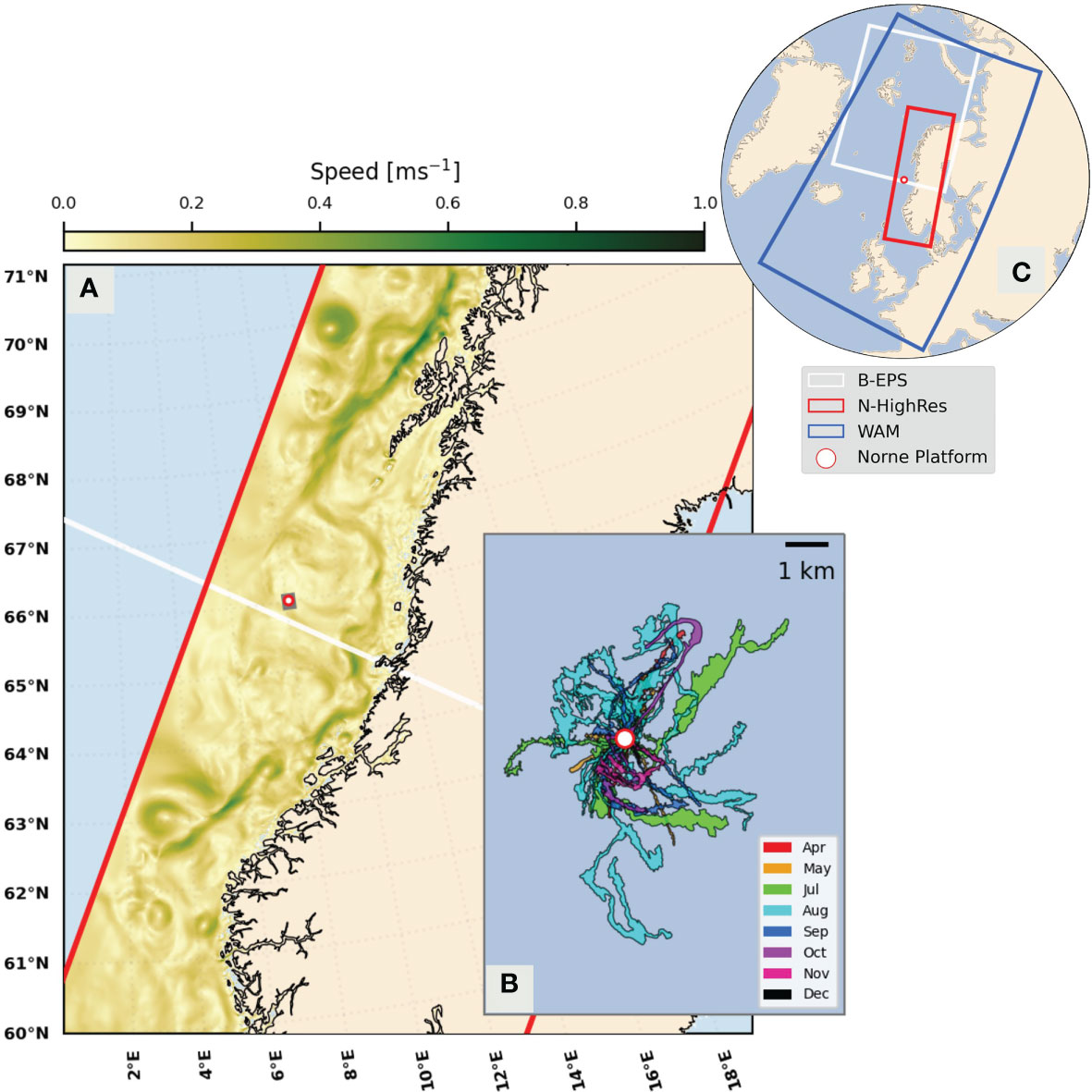
Figure 1 Overview of the area of study. (A) Location of the Norne platform (dot) offshore the Norwegian coast. The colormap in represents the N-HighRes ocean current speed (ms ⁻¹) averaged between the 1st and 14th of April, 2021. The grey polygon around the platform is zoomed-in in (B), with the delineated PW slicks for each month. Red and white lines depicts the grid domain of N-HighRes and B-EPS. Their full extent, including the WAM domain (blue), can be seen in (C).

2.2 Produced water and in situ wind data

According to the national regulations, PW discharge on the Norwegian shelf is legal provided that the monthly average oil concentration does not exceed 30 gm⁻³ (Miljørapport, 2019). When the platform is operational PW is continuously released from a sub-surface pipe from which the oil rises to the surface. The release volume and concentration vary over time, though the variability is on a bi-weekly to monthly time scale. Release data from the Norne platform in 2021 was provided by the operator and the average daily PW oil release was 253 kg, average water release was 19754 m³, with an average oil concentration of ∼ 10.85 gm⁻³ and an average flux of 0.23 m³ s ⁻¹. The oil volume percentage of 0.013% means that it is classified as an oil-in-water type of emulsion (Lu et al., 2020), though such low concentrations put the releases close to the oil free water surfaces. Damping ratio, relative thickness, estimates of produced water slicks indicates low variability and hence confirm the assessment of thin surface slicks (Skrunes et al., 2019; Johansson et al., 2021).

Wind speed and direction are recorded every 3 hours at Norne. Observations between April and December 2021 were used to assess the modeled winds of Barents 2.5-EPS and NorKyst-800 through the Root Mean Square Error (RMSE), bias and Willmott skill score (Willmott, 1981, WS). The alignment between observed wind direction and the PW bearing angle was also verified in order to evaluate the role of winds on the transport of the PW slicks. The findings are presented in Section 3.1.2.

2.3 Geophysical forcing

Norne is located in the Norwegian continental shelf, bordered by the Norwegian Coastal Current (NCC) flowing northward alongshore and by the Norwegian Atlantic Slope Current (NwASC) along the continental slope. The region is generally considered mesoscale eddy rich, with stable dynamic boundaries on the continental slope preventing cross-shelf transport (Dong et al., 2021). The abundance of eddies can also be observed in Figure 1A. The existence of density fronts in the region is known (Dong et al., 2021), and turbulent baroclinic instabilities might affect the PW drift.

2.3.1 Ocean model ensemble

Ocean currents are provided by two regional setups of the Regional Ocean Modeling System (ROMS, (Shchepetkin and McWilliams, 2005)): The Barents 2.5-EPS (B-EPS) ocean model provides a 6-member ensemble with 2.5 km horizontal resolution (B-EPS), and the NorKyst-800 (N-HighRes) ocean model provides deterministic forecasts at higher resolution of 800 m (Figure 1). B-EPS is a coupled ocean-ice system for the Barents Sea and Northern Norway and N-HighRes is a regional model for the entire coast of Norway. The model domains overlap at the experiment site and provide daily forecasts with 66 hrs lead time.

B-EPS is initialized each day from the forecast of the previous day, with update increments provided by an Ensemble Kalman filter data assimilation scheme (Sakov and Oke, 2008). While sea surface temperature and in-situ hydrography are assimilated to constrain the density fields, no data that directly constrains the velocity fields is being assimilated. Details on the configuration for B-EPS model are given in (Röhrs et al., 2023b). In principle, ensemble spread in B-EPS is maintained by forcing of the ocean model with an atmospheric ensemble. The first is forced by a high-resolution weather forecast model AromeArctic (Müller et al., 2017a) (2.5 km x 2.5 km), while the subsequent members are forced by random members of the ECMWF-ENS forecast (ECMWF, 2012). In addition, each ensemble member retains their identity from the previous forecast cycle. Consequently, as the current field develops independently in each member the B-EPS ensemble permits various realizations of mesoscale circulation across the members. While ensemble spread of SST is validated in Röhrs et al. (2023b), spread in surface circulation and the ability of the ensemble to represent uncertainties in currents are the subject of ongoing investigations.

N-HighRes is a regional ocean model covering the whole Norwegian coast at an eddy-resolving resolution. The model is forced by the atmospheric forecast model Arome-MEPS (Müller et al., 2017a). Details of N-HighRes are provided in Asplin et al. (2020) and references therein.

While B-EPS assimilates sea surface temperature and sparse in-situ data, neither of the two ocean models exhibits constraint of mesoscale ocean circulation that directly provides forecast skill in surface currents. A degree of predictive skill in ocean surface currents may however arise by the relatively high degree of predictability in the used wind forcing.

Both model setups include the major tidal constituents provided by TPXO 7.2, and receive lateral boundary conditions from the TOPAZ4 hydrodynamic model (Xie et al., 2017). TOPAZ4 has a horizontal resolution of about 10 km, it is based on the Hybrid Coordinate Ocean model and is part of the Copernicus Marine Environment Monitoring Service for the Arctic domain.

2.3.2 Atmospheric forcing ensemble

While each of the used ocean model representations receives different atmospheric forcing, the wind from the respective model is also a direct input for the oil drift simulations, as surface slicks become direct subject to atmospheric drag.

AROME-Arctic and Arome-MEPS (hereinafter AROME) are the regional high-resolution weather prediction models for the Barents Sea and Norway, respectively. Both systems issue weather forecasts 66 hrs ahead with multiple update cycles each day. AROME is based on the HARMONIE-AROME model configuration of the ALADIN-HIRLAM system (Bengtsson et al., 2017), with boundary conditions obtained from ECMWF’s IFS.

2.3.3 Wave prediction model

A prognostic model for the evolution of the wave energy spectrum, WAM (Komen et al., 1994), is used to calculate Stokes drift and wave entrainment rate of surface oil. The used implementation of WAM at MET Norway has a horizontal resolution of 4 km, resolving the wave energy spectrum in 36 directions and 36 frequencies (Gusdal and Carrasco, 2012). The Stokes drift is calculated from significant wave height, peak period and the wave direction according to Breivik et al. (2014), hence taking into account both wind sea and swell contributions to the depth-dependent Stokes drift profile. While surface oil slick is advected by the surface Stokes drift, submerged oil particles are moved by the Stokes drift at the respective particle depth.

2.4 Oil drift model - OpenOil

The open-source oil transport and weathering Lagrangian framework, OpenOil, is used to perform the drift simulations (Röhrs et al., 2018). Embedding tabulated oil information provided by the Norwegian Clean Seas Association for Operating Companies (NOFO) and linked to the ADIOS oil library (https://github.com/NOAA-ORR-ERD/PyGnome), OpenOil is part of the OpenDrift Lagrangian particle tracking model (Dagestad et al., 2018).

Oil surface transport in OpenOil is formulated as presented in Eq. 1. The wind drift factor (α) was fixed at 3%. The releasing point is located at 12 m depth and it takes around four minutes for the PW to reach the ocean surface. We initialise the drift simulations at the ocean surface.

OpenOil distinguishes between submerged droplets and elements that are part of a surface slick. Redistribution between these reservoirs is controlled by buoyancy, wave entrainment and vertical mixing (Nordam et al., 2019). Buoyancy depends on oil droplet density and the particle size. The droplet radius distribution depends on the viscosity, interfacial tension and wave dissipation as parameterized according to Li et al. (2017). Entrainment of surface particles is parameterized as function of wave energy dissipation from the wave model, using empirical relationships provided by Li et al. (2017). Further details on the implementation of surface interaction of particles and their behavior in the turbulent water column are given in Röhrs et al. (2018).

2.5 Simulation setup and evaluation

For each PW delineated from the SAR scenes, simulations were started 6 hrs before the acquisition time and ran for this same time interval. The ensemble simulations were performed using the ocean and atmospheric fields provided by the B-EPS, while N-HighRes forcing was used for the deterministic runs. In both cases, Stokes drift was imported from WAM, where the e-folding depth decay is calculated according to (Breivik et al., 2016). Two setups were defined in this work: (Setup 1) Simulations including ocean forcing, Stokes drift and the wind fields, and (Setup 2) Simulations forced solely by the wind fields. Weathering processes were not considered in the simulations.

The evaluation is divided into three different approaches, namely Member-wise Assessment, Model Comparison and Ensemble Verification. These are described below.

2.5.1 Member-wise assessment

The 656 model results (41 scenes, 8 simulations per scene and 2 setups) were evaluated against their respective PW observations (member-wise assessment). As these are simple snapshots and not time series of PW displacement, commonly used skill scores (e.g. the normalized cumulative Lagrangian separation (SS), Liu and Weisberg (2011)) are not applicable. We therefore considered two recently proposed metrics by Dearden et al. (2022) for instantaneous observations, the Centroid Skill Score $\left({\text{C}}_{SS}\right)$ and Area Skill Score $\left(A_{SS}\right)$:

$\begin{array}{ll}{C}_I=\frac{\Delta x}{L_{OBS}}& (2)\end{array}$

where Δx is the distance between predicted and observed centroids at a given time instance and L_OBS is the length of the observed oil spill. The C_SS is defined as:

$\begin{array}{ll}{\mathcal{C}}_{\mathcal{S}\mathcal{S}}=\{\begin{array}{ll}1-\frac{C_I}{C_{thr}},\hfill & \text{for\hspace{0.17em}}{C}_I<C_{thr}\hfill \\ 0,\hfill & \text{for\hspace{0.17em}}{C}_I>C_{thr}\hfill \end{array}& (3)\end{array}$

where ${\text{C}}_{thr}$ is a tolerance threshold defined by the user. The ${\text{A}}_{SS}$ is defined similarly as:

$\begin{array}{ll}{A}_I=\frac{\left|A_{PR}-A_{OBS}\right|}{A_{OBS}}& (4)\end{array}$

which is simply the absolute difference between the predicted and observed oil spill areas, normalized by the observed area. The area skill score is then defined as:

$\begin{array}{ll}{\mathcal{A}}_{\mathcal{S}\mathcal{S}}=\{\begin{array}{ll}1-\frac{A_I}{A_{thr}},\hfill & \text{for\hspace{0.17em}}{A}_I<C_{thr}\hfill \\ 0,\hfill & \text{for\hspace{0.17em}}{A}_I>C_{thr}\hfill \end{array}& (5)\end{array}$

A ${\text{C}}_{thr}$ value of 1, adopted in Eqs. 3 and 5, means that the model to present any skill, the predicted parameter must not exceed the magnitude of its observed counterpart. One would obtain a perfect skill score if both ${\text{C}}_{SS}$ and ${\text{A}}_{SS}$ = 1.

Setting the tolerance threshold is not trivial and it was previously shown to being sensible to the forecast horizon (Révelard et al., 2021) and region under investigation (de Aguiar et al., 2022). For this reason, two other metrics were applied, namely the centroid distance error ($\text{Δ}x$ in Eq. 2) and offset angle (OA). The latter is the angle between modeled and observed centroids, ranging from $0^{\circ }$ to $\pm$ ${180}^{\circ }$.

Figure 2 illustrates the verification approach. Each color represents trajectories forced by one of the eight different forcing fields, and the highlighted points are their respective centroids. Considering N-HighRes output as an example, the distance error between observed (red dot) and modeled (white) centroids is depicted as the solid black line ($\text{Δ}x$, centroid distance error) whereas the angle between the two orange lines represents the offset angle.

FIGURE 2

Figure 2 Example of PW slick simulation. The solid yellow area represents the SAR derived PW slick. Outputs forced by the different ocean-atmospheric models are shown with different colors (see legend). The white ellipse represents the 2 std confidence ellipse (CE) for N-HighRes, and modeled centroids are shown as highlighted dots. The mean B-EPS CE is shown as the pale green ellipse. The solid black line represents the distance error between the PW centroid (solid red dot) and the N-HighRes centroid (white dot), and the offset angle between them is represented by the solid black sector. Simulations are initialized at the Norne location (white-cross purple dot). Note that the N-HighRes covers only a segment of the delineated PW slick (solid red shape).

2.5.2 Model comparison and ensemble verification

The member-wise metrics ($C_{SS}$, $A_{SS}$, centroid distance error and offset angle) do not provide information of the quality of the ensemble system. Confidence ellipses (CE) are often used in ensemble modeling as a proxy of spread. We therefore consider CEs as follows: the cloud of particles follow a two-dimensional Gaussian distribution. Two-standard deviation ellipses were fitted for each of the model outputs, and the area of these were used in $A_{SS}$ (Eqs. 4 and 5). An additional CE was fitted considering all ensemble members (mean EPS). This is illustrated in Figure 2 as ellipses enclosing each forcing with their respective colors, and a pale-green ellipse representing the mean EPS.

As the mean ensemble CE can be inflated to the point that it will likely cover the observed PW slick, we also evaluated the performance of the EPS by counting the number of observed centroids that fall within the mean EPS CE domain (hit). The relation between the area of the latter and the separation distance between modeled and observed centroids was also inspected.

For a model with statistical skill, the forecast results and the observed true state – the verification – ought to be independent draws from the same probability distribution, which may be evaluated in terms of a model and observation value histogram. In addition, the spread in forecast results among a $N$-member EPS is supposed to reflect the actual uncertainty in forecasts. Rank histograms and the spread-error relation are used to determine the ensemble spread. By definition, a rank histogram is built on $N+1$ bins (Hamill, 2001). For each observed centroid position, its longitude and latitude is verified against the ranked ensemble members coordinates. A well-calibrated ensemble system evaluated at many independent cases ought to provide a uniform rank histogram, while overdispersive (underdispersive) systems will present a concave (convex) distribution. For 2D rank histograms, these distributions are seen as homogeneous, centered and clustered in the corners, respectively.

Spread (s) and error ($ϵ$) are hereby defined as the square root of the average ensemble variance and the root mean square error of the ensemble mean ($\overline{X}$) (Eckel and Mass, 2005), respectively. The latter is simply the ensemble mean position and it is defined as:

$\begin{array}{ll}\overline{X}=(\frac{1}{N_{x,y}}){\displaystyle \sum _{n=1}^N{X}_{x,y}}& (6)\end{array}$

where N is the number of ensemble members and x,y represents all the longitude and latitude positions of the virtual particles (X). The spread s is given by:

$\begin{array}{ll}s=\sqrt{\frac{1}{M}{\displaystyle \sum _{m=1}^M\left(\frac{1}{N-1}{\displaystyle \sum _{n=1}^N{({\overline{X}}_{N_{x,y}}-\overline{X})}^2}\right)}}& (7)\end{array}$

where ${\overline{X}}_{N_{x,y}}$ is the mean position of a given ensemble member and M is the number of observations. The error ($ϵ$) is then defined as:

$\begin{array}{ll}ϵ=\sqrt{\left(\frac{N}{N+1}\right)\frac{1}{M}{\displaystyle \sum _{m=1}^M{(\overline{X}-P{W}_{x,y})}^2}}& (8)\end{array}$

where ${\text{PW}}_{x,y}$ is the observed PW centroid. Similarly to the rank histogram, the spread-error relationship also indicates if the EPS addresses uncertainties correctly ($ϵ\approx$ s), if it overestimates ($ϵ<<$ ts) or underestimates them ($ϵ>>$ s). To examine the role of the wind field on the modeled PW slick drift, we conducted the same analysis on simulations solely wind-forced (Setup 2). The work design is illustrated in Figure 3.

FIGURE 3

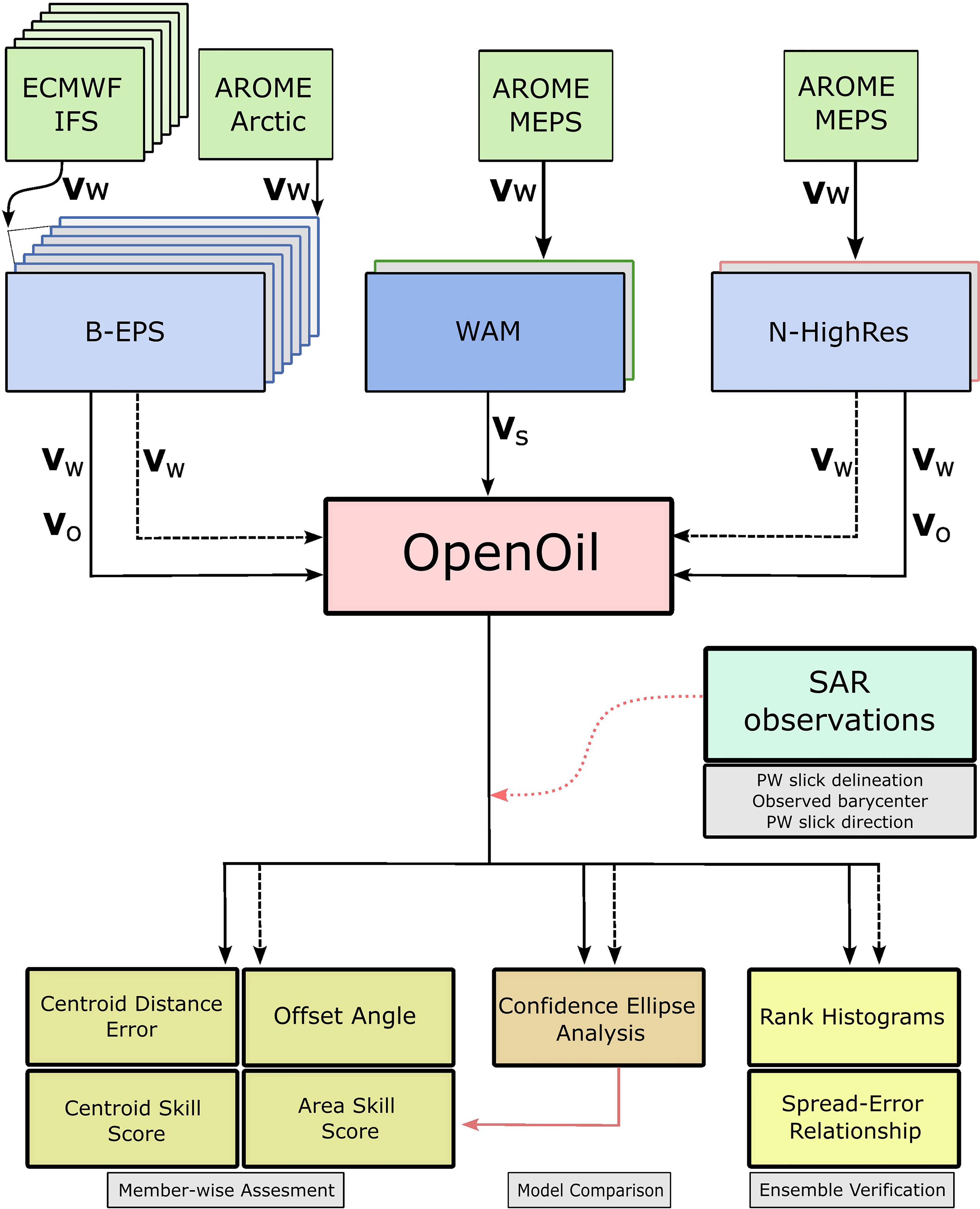
Figure 3 Flow chart representing the work design. Blue blocks: the three model products considered in this study as inputs. Dashed arrows represent simulations wind forced $({\text{V}}_w$, Setup 2) while the solid lines symbolize a combination of ocean currents $({\text{V}}_o$), Stokes drift $({\text{V}}_s$) and the wind field (Setup 1). Red block: OpenOil, the Lagrangian modeling framework. Green block: Observed PW slicks, their centroids and drift direction obtained from Sentinel-1A/1Bscenes. Yellow blocks: Evaluation (Member-wise Assessment, Model Comparison and Ensemble Verification).

3 Results

3.1 PW drift simulations

3.1.1 Observed and modeled overall distributions

Heatmaps of the observed slicks, and contours representing simulations for Setup 1 (magenta) and Setup 2 (black), for B-EPS (a) and N-HighRes (b), respectively, are shown in Figure 4. Their latitudinal (right sub-panel) and longitudinal (top sub-panel) probability densities are also displayed. One can notice that the B-EPS for Setup 1 presents the highest spread and its distributions fit well to the observed. The results also indicate that differences between the two set of simulations for N-HighRes are not as pronounced as for the ensemble system.

FIGURE 4

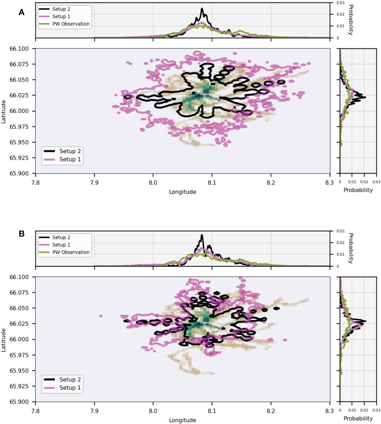
Figure 4 Distribution of observed (heatmap) and modeled (contours) slicks. Magenta (black) represents Setup 1 (Setup 2) simulations. Outputs in panel (A) were obtained with B-EPS and (B) with N-HighRes. The top and right sub-panels show the longitudinal and latitudinal distributions following the color legend.

The mean latitude and longitude positions were centered around the releasing point, as expected. The ratio between observed (Obs.) and modeled (Mod., B-EPS and N-HighRes) standard deviations of the probability distributions (P) for Setup 1 and Setup 2 are shown in Table 1. The results indicate that virtually no difference exists between B-EPS and N-HighRes in Setup 2. Including the ocean fields, increased the standard deviation in both models, with B-EPS presenting slightly better overall performance.

TABLE 1

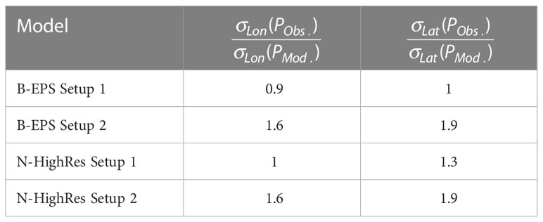
Table 1 Standard deviation ($\sigma$) ratio between observed (Obs.) and modeled (Mod.) for longitudinal and latitudinal probability distributions (P) in Figure 4.

3.1.2 Member-wise assessment of modeled PW drift

The member-wise assessment for Setup 1 are shown in Table 2 and for Setup 2 in Table 3. N-HighRes presented slightly better performance than the EPS members in every metric but ${\text{A}}_{SS}$. One can further notice that all models have negative OA values, meaning that the modeled centroid is located to the left of the observed ones. Setup 2 provided better results for all metrics considered relative to Setup 1, with lower variability in the outputs. As for Setup 1, the modeled slicks presented a counterclockwise rotation relative to the observations.

TABLE 2

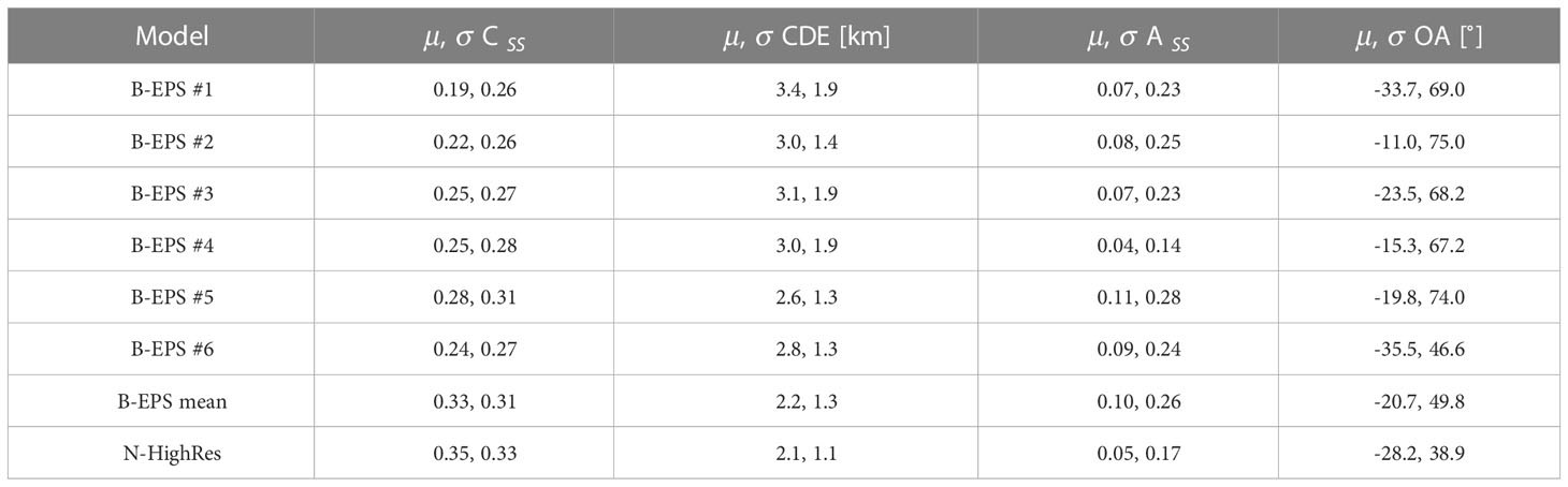
Table 2 Mean ($\mu$) and standard deviation ($\sigma$) of the Centroid Skill Score $\left({\text{C}}_{SS}\right)$, Centroid Distance Error (CDE, km), Area Skill Score $({\text{A}}_{SS}$) and Offset Angle (OA, ^∘) for Setup 1.

TABLE 3

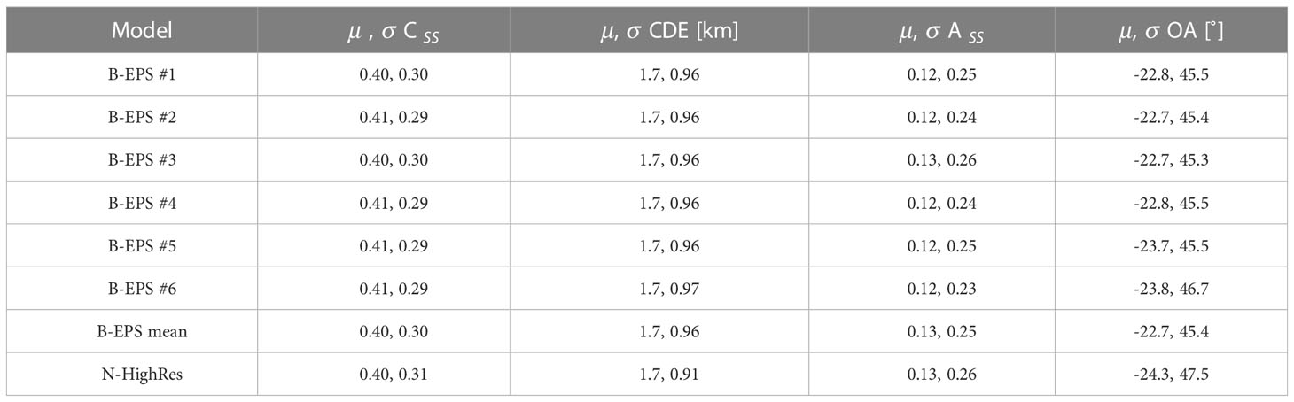
Table 3 Same as Table 2, but for only wind forced simulations (Setup 2).

3.2 PW slick drift and wind direction

The modeled slicks, whether including ocean forcing or not, are predominantly rotated anticlockwise relative to the observations. This finding indicates that the atmospheric models exhibit a consistent bias. We show in Figure 5 the polar histograms of speed and direction errors between modeled (B-EPS member 1 (a); N-HighRes (b)) and observed winds. Both models slightly overestimate the wind speed, presenting a mean error (${\mu }_{Dif{f}_{spd}}$) of 0.92 ms ⁻¹ and 1.23 ms ⁻¹, respectively. Modeled winds are rotated clockwise relative to the observations, having N-HighRes a lower mean wind direction error (9.8∘) compared to B-EPS member 1 (21.3∘). About 44$\%$ and 50$\%$ of the observations fall within the bounding boxes, respectively. A summary of the evaluation can be seen in Table 4.

FIGURE 5

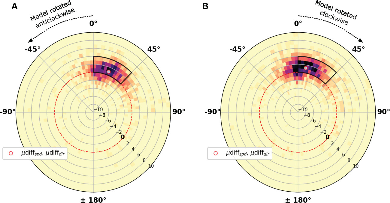
Figure 5 Polar heatmaps of wind speed (radius, m s ⁻¹) and direction (angle) errors between model $({\text{V}}_{wm}$) and observation $\left({\text{V}}_{wo}\right)$, Apr - Dec 2021. (A) for B-EPS member 1 and (B) for N-HighRes. Positive angles represent modeled winds rotated clockwise relative to the observed wind direction and positive values in radius indicate ${\text{V}}_{wm}>$ ${\text{V}}_{wo}$. The red dashed line indicates where ${\text{V}}_{wm}=$ ${\text{V}}_{wo}$, the white dot indicates the mean speed and mean direction errors for each model and the black polygon the region of highest concentration.

TABLE 4

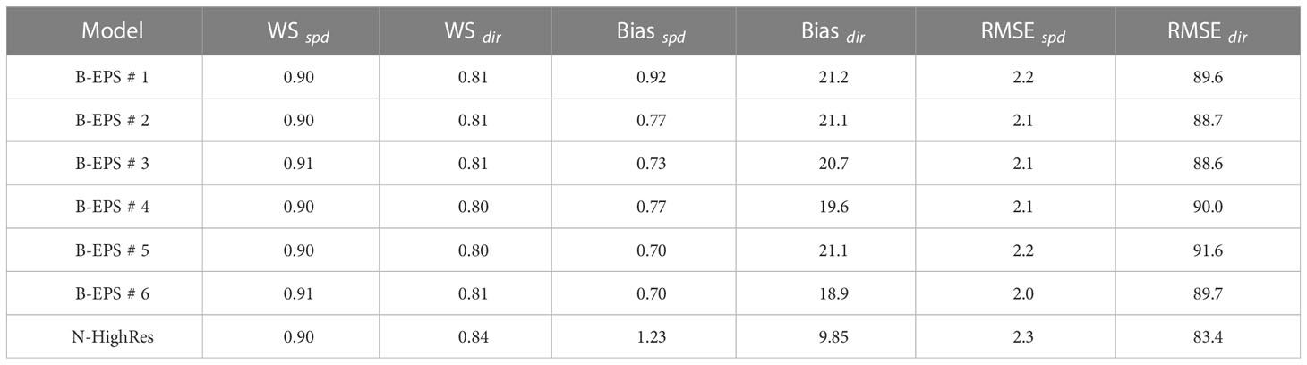
Table 4 Willmott Skill (WS), Bias and Root Mean Square Error (RMSE) for wind speed (spd) and direction (dir). Each atmospheric product was assessed relative to wind observations at Norne between April and December, 2021.

The mismatch between observed wind direction and PW bearing angle is shown in Figure 6A. Due to gaps in the wind time series between April and June, 28 scenes were assessed instead of 41. Twenty-three of these presented deflection greater than 0^° relative to the observed wind direction, with the majority being concentrated between 30^° and 45^°. An illustrative representation of the results is show in Figure 6B.

FIGURE 6

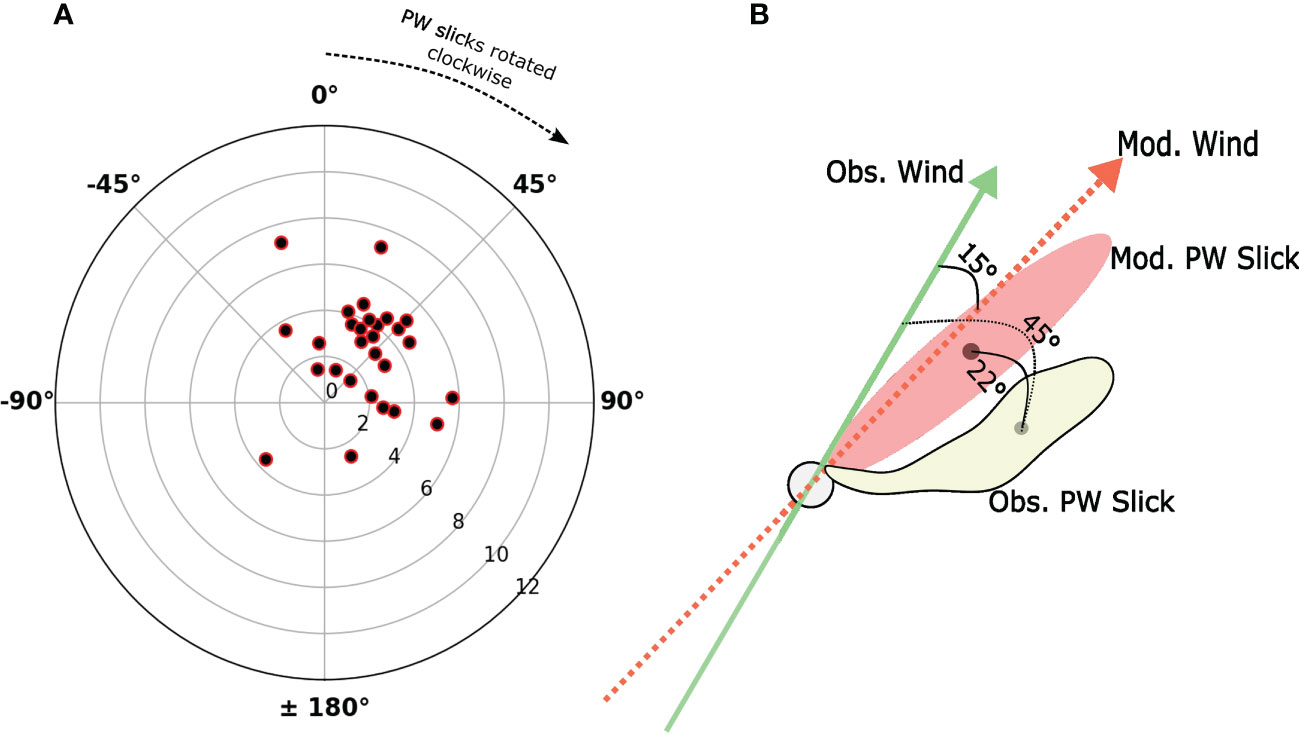
Figure 6 (A) Offset angle between observed PW centroid and observed wind directions. Radius values indicate the observed wind speed (ms ⁻¹). (B) Schematic illustration of the slick deviation, where modeled slicks (Mod. PW Slick) veered counterclockwise ($\approx$22^∘) relative to the observed slicks (Obs. PW Slick). The latter were deflected about 45^∘ to the right of the observed wind (Obs. Wind). Modeled winds (Mod. Wind) were veered clockwise around 15^∘ relative to Obs. Wind.

3.2.1 Model comparison

The area covered by the mean EPS CE gives an indication of the members spread. Tables 5, 6 show the average ($\mu$), standard deviation ($\sigma$) of the CE areas, and the number of hits (Hits) of each model product for Setup 1 and Setup 2, respectively. The results clearly show an increase in the average extent of all CEs with the inclusion of ocean currents and the Stokes drift in the simulations (Setup 1). One can further notice that the Setup 2 mean B-EPS CE shows virtually no difference of $\mu$ and $\sigma$ values relative to the B-EPS members, in contrast to Setup 1 (about four-times higher).

TABLE 5

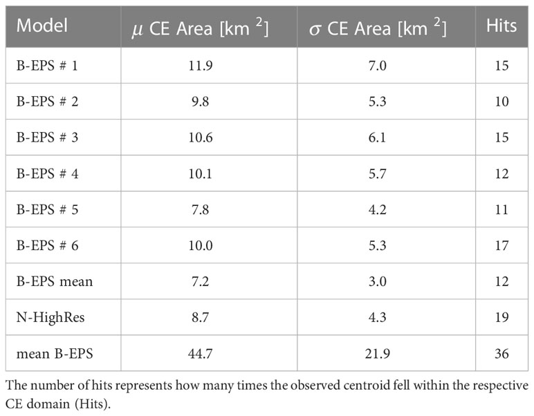
Table 5 Average ($\mu$, km²) and standard deviation ($\sigma$, km²) of the confidence ellipse area (CE) of each model product and the mean B-EPS for Setup 1.

TABLE 6

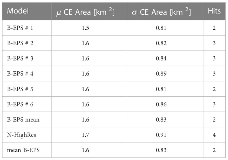
Table 6 Same as Table 5, but for Setup 2.

The average (std) ratio between the mean EPS and the members CE’s areas for Setup 2 was estimated to 0.99 (0.05), and 0.26 (0.17) for Setup 1. Additionally, the ensemble members had an average area about 30$\%$ (0.01$\%$) higher (smaller) than N-HighRes for Setup 1 (Setup 2).

The mean EPS CE for Setup 1 also presented the highest number of hits (36), 46% higher than N-HighRes. This could indicate that the CEs are simply inflated to the point that their area are more likely to encompass the observations, but the average distance error between the confidence ellipse center and the observed PW centroid was 2 km. For Setup 2, only 2 (4) hits were registered for N-HighRes (mean B-EPS).

3.2.2 Ensemble verification

Figure 7 shows the rank histograms of Setup 1 (A) and Setup 2 simulations (B), respectively. Panels (C–E) are examples of overdispersive, consistent and underdispersive rank histograms created from synthetic data randomly sampled from Normal distributions with the same mean (0) and decreasing standard deviation (10, 1, 0.1). Comparing these to the obtained results, it is possible to notice the resemblance between Setup 2 rank histograms (B), and the underdispersive case (E), and Setup 1 (A) with panel (D).

FIGURE 7

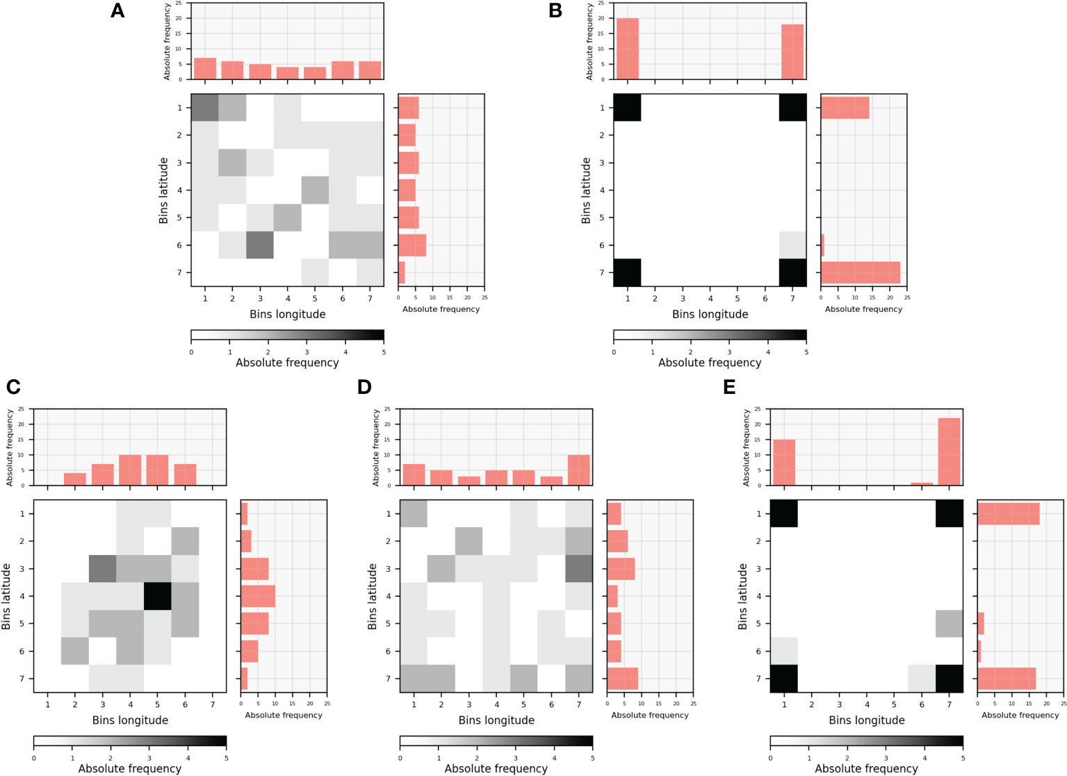
Figure 7 Two-dimensional rank histograms of B-EPS for Setup 1 (A) and Setup 2 (B) in absolute frequency. Panels (C–E) represent overdispersive, consistent and underdispersive rank histograms created from synthetic data randomly sampled from Normal distributions with the same average (0) and decreasing std (10, 1, 0.1), respectively. Top and right sub-panels show the longitudinal and latitudinal rank histograms.

The ratio between error (ϵ) and spread (s) (Eqs. 7 and 8) for an ideal ensemble system should be approximately 1. The previous findings are supported by $\frac{ϵ}{s}\approx$ 1.3 for Setup 1 and $\frac{ϵ}{s}\approx$ 69 for Setup 2.

4 Discussion

4.1 Representation of PW slick drift using ocean forecast models

The results presented in the previous section indicate that the EPS reproduced the overall variability of PW slick drift (Figure 4) and performs similarly to N-HighRes in a member-wise level (Tables 2, 3). The skill scores obtained for the latter are on average slightly higher than for B-EPS, though the difference is small, especially when considering the ensemble mean. It is also worth noticing that the Centroid Skill Score and Area Skill Score did not present sensitivity relative to ‘bad’ simulations (e.g., Figures 8C, F), whereas the unskilled predictions were addressed as skillful (not shown). We stress that our work did not attempt to model the shape of the slicks as they are too narrow (between 85 m to 200 m) to be resolved by the operational models.

FIGURE 8

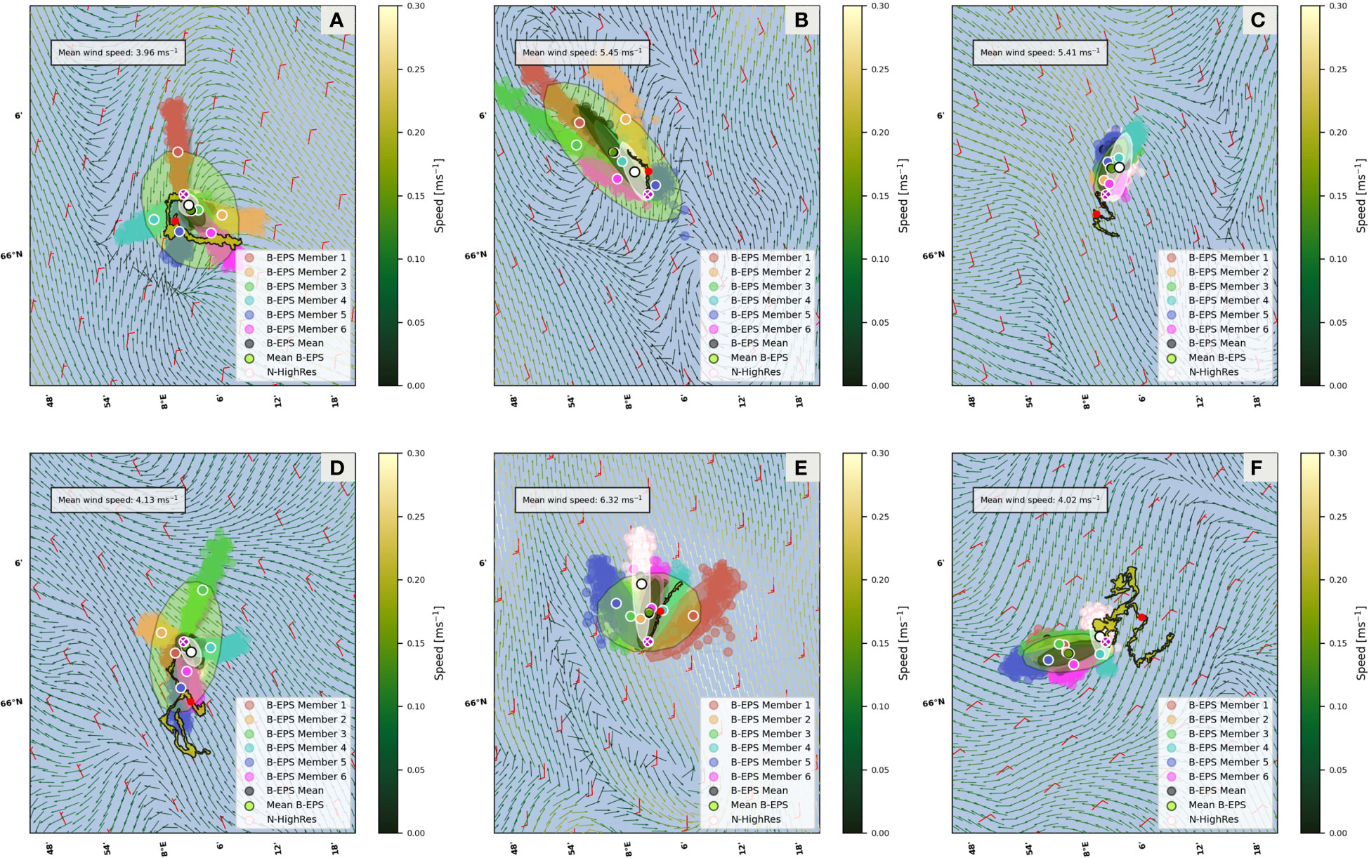
Figure 8 Example of high spread, partially accurate (A, D); low spread, accurate (B, E) and low spread, inaccurate (C, F) simulations. The white-crossed, magenta dot represents Norne. Wind barbs (red) and ocean current vectors with superimposed speed (colormap, ms ⁻¹) were obtained from N-HighRes. The modeled mean wind speed (ms ⁻¹) is also shown on the top left box. Respective Figures for all 41 PW slick drift cases are provided as electronic supplement to this document.

For their short spatial and temporal scales, PW slicks are highly influenced by higher frequency, evanescent small scale features with life spans from less than 5 hrs (Kirincich, 2016) to shorter than he inertial period (Callies et al., 2020). These phenomena are unconstrained by current observation systems, resulting in lower predictive skill of higher resolution models (Sandery and Sakov, 2017; Jacobs et al., 2021).

Eddy-resolving ocean models may directly improve the statistics of Lagrangian currents due to their better representation of the kinetic energy spectrum at small scales. However, the use of high-resolution ocean models may not translate into improved predictive skill due to misrepresentation of the circulation features in space or time (Révelard et al., 2021). Neither B-EPS nor N-HighRes are expected to exhibit predictive skill for surface currents beyond wind-driven and bathymetry-constrained flow, but rather represent uncertainties in such unconstrained scales.

4.2 Modeling oil drift using ensemble forecasting

Confidence ellipses have been used as an indirect tool by the atmospheric community for the assessment of ensemble spread for more than a decade. In our analysis, we found a 36/41 (≈87.8%) hit ratio for the ensemble simulations in Setup 1. This is fairly close to the theoretical value of 86.5$\%$ associated to the considered two standard deviations confidence interval (Wang et al., 2015). The discrepancy of $\mu$ between B-EPS members and the mean B-EPS CE areas for Setup 1 (see Tables 5) entails from diverging trajectories, otherwise, the average mean B-EPS CE area should be roughly similar to those of the ensemble members. We therefore stress that the mean EPS CE areas are not arbitrarily inflated, but their growth rather reflects the B-EPS spread induced by the uncertainties in the ocean field. Converging to Melsom et al. (2012) and Sandu et al. (2020) findings, we also observed slightly better accuracy of the mean EPS CE (2 km) relative to N-HighRes (2.1 km).

Despite showing better performances in all member-wise metrics, Setup 2 results are indistinguishable among the distinct model products (see Tables 1, 3 and 6). Such lack of variability stems from higher homogeneity of atmospheric horizontal flows in comparison to the ocean (Figure 2), i.e., the simulated trajectories experience essentially alike wind conditions. Additionally, due to horizontal (500 km) and temporal (6 hrs) decorrelation scales adopted on ECMWF-ENS’s perturbation schemes, the ensemble spread of winds is generally low at the spatial (1-15 km) and temporal (1-6 hrs) ranges investigated here. We acknowledge that uncertainties in the wind field are the main sources of variability in large and persistent oil slick scenarios (e.g. Li et al., 2019; Kampouris et al., 2021), but we have evidences that it is overridden by the ocean currents on short scales.

These findings corroborate with the rank histograms (Figure 7). The uniform- and cornered-like patterns obtained for Setup 1 and Setup 2, respectively, fits the artificial examples of consistent and underdispersive cases. A uniform histogram is a necessary, but not sufficient condition for determining the reliability of an ensemble system due to conditional biases, nonrandom sampling or low number of samples (Hamill, 2001). For finite size ensemble systems, the ideal error-spread ratio is altered by an adjusting factor $\frac{ϵ}{s}=$ 1 + $\sqrt{\frac{2}{N-1}}$, $\approx$ 1.2 for N $=$ 6 (Eckel and Mass, 2005). The error-spread ratio analysis confirmed that Setup 2 simulations presented a value ($\frac{ϵ}{s}\approx$ 69) overly above the desired ($\frac{ϵ}{s}\approx$ 1.2). Taking into account the ocean currents and the Stokes drift greatly improved the spread among the EPS members, resulting in $\frac{ϵ}{s}\approx$ 1.3. Despite the proximity of the releasing location to the boundary domain ($\approx$ 30 km), these results show that the ensemble spread in surface currents is readily developed at the study region.

Due to the number of possible future states that EPS provide, often exceeding 20 members, ensemble modeling has been used by weather prediction centers to forecast the strength, probability of occurrence and regions impacted by hazardous events. Figure 8 shows examples of PW drift simulations with different degrees of ensemble spreading. Panels (B, C) and (E, F) illustrate cases where particles follow a well-defined path and responders can have higher confidence to base their decision plan. Note that low spread does not necessarily imply accurate predictions as all the members can converge to a wrong predictions (Figures 8C, F). Decision making is hindered in the case that simulations diverge or present bifurcations, as shown in Figures 8A, D. In this case, the drift uncertainty is higher and this leads to a more problematic recovery/rescue planning.

4.3 The misalignment between observed slicks and the wind direction

An offset in the drift direction between modeled and observed slicks was found for both Setup 1 and 2. Such mismatch can result from circulation features not resolved by the ocean model, but also from errors in the description of Ekman transport in the boundary layer schemes for both the ocean and the atmosphere models (Sandu et al., 2020) The latter is evidenced in Figure 5 and Table 4 as bias in wind speed and direction, leading to the observed systematic offset in drift directions for the oil slick simulations

Stokes drift (Röhrs et al., 2012), Langmuir circulation (Yang et al., 2014) and wave-current interactions (Staneva et al., 2021) were shown to impact drift trajectories and improve predictive skill when included. While the Stokes drift is explicitly included in the trajectory simulations, the used ocean and wave model setups are not coupled, meaning that wave-current interactions are not represented in the ocean model (Geernaert, 1993; Chen et al., 2020). The influence of these phenomena are small when considered independently, but introduce further errors on short-term predictions not accounted for in operational models. The Stokes drift has been shown to have an important contribution to surface slick motion, as discussed in Röhrs et al. (2012); Jones et al. (2016); van den Bremer and Breivik (2018).

Trajectory models are at the endpoint of a complex chain of observation systems and forecast models. Beyond the impact of internal and external sources of uncertainties (Barker et al., 2020), drift modeling is also sensible to releasing time (Li et al., 2019). Although released constantly, the residence time of PW slick at the ocean surface is unknown, hence the considered forecast time (6 hrs) is arbitrary. Another drawback of this study is related to the delineation process as this depends on the operator experience and it is subjective. We recommend that further investigations on drift ensemble modeling should link remotely-sensed observations and in-situ data, preferably oil droplet diameter and drifter trajectories. It would also be useful to test the influence of perturbations in the model physics, boundary conditions and wave-ocean interactions on the drift modeling.

5 Concluding remarks

Here we assessed the capability of an ocean ensemble model (B-EPS) to represent oil slick drift and its uncertainty, compared to a higher resolution deterministic ocean model (N-HighRes). The simulated trajectories were conducted with the open-source Lagrangian framework OpenDrift, and forced by these two ocean models in addition to wind forcing and Stokes drift (Setup 1). The predictions were evaluated against Produced Water slicks delineated from 41 Sentinel-1A/1B scenes over the Norne platform between April and December, 2021. Three approaches were considered for the verification: Member-wise Assessment, Model Comparison and Ensemble Verification. The importance of the wind field on the modeled trajectories was also investigated by forcing the virtual particles only with atmospheric models (Setup 2).

Produced water slicks are thin films with low oil concentrations, generally observed as narrow stripes and lasting for a short period. For short range predictions as considered here (6 hrs), we showed that simulations forced solely by the wind fields are underdispersive. For larger and more persistent slicks, the wind forcing may still be considered the main source of variability.

Despite its coarser horizontal resolution, the ensemble prediction system, and especially its mean field, presented similar member-wise results relative to the deterministic ocean model. We have also shown that the observed PW drift presented a consistent clockwise deviation from modeled and observed wind directions, possibly resultant from systematic errors in the description of boundary layer schemes and wave-current interactions not resolved in the used models. The analysis of confidence ellipses and distributions of drift patterns show that realistic drift modeling requires to include both the ocean and wind forcing, and analysis of ensemble spread indicates that including the currents is necessary to properly address uncertainties in drift modeling.

Data availability statement

All geophysical forcing data is available at https://thredds.met.no/thredds/catalog.html and the level 1 Sentinel-1A/Sentinel-1B data are available at https://creodias.eu/. Wind measurements are freely available at https://seklima.met.no/. OpenDrift can be downloaded at https://opendrift.github.io/. Produced water slick masks can be provided upon request.

Author contributions

Study design and conception: VA, JR, AJ, and TE. Organization of SAR database: VA. Trajectory simulations and analysis: VA. Produced water data set and analysis: AJ. Manuscript initial draft: VA. Manuscript editing: all authors. All authors contributed to the article and approved the submitted version.

Funding

This work was supported by the Research Council of Norway (RCN) project Center for Integrated Remote Sensing and Forecasting for Arctic Operations (CIRFA) (237906).

Acknowledgments

Copernicus Sentinel data 2021 for Sentinel data. Equinor is gratefully acknowledged for providing data about produced water releases from the Norne platform. We thank the reviewers for the constructive comments and suggestions.

Conflict of interest

The authors declare that the research was conducted in the absence of any commercial or financial relationships that could be construed as a potential conflict of interest.

Publisher’s note

All claims expressed in this article are solely those of the authors and do not necessarily represent those of their affiliated organizations, or those of the publisher, the editors and the reviewers. Any product that may be evaluated in this article, or claim that may be made by its manufacturer, is not guaranteed or endorsed by the publisher.

Supplementary material

The Supplementary Material for this article can be found online at: https://www.frontiersin.org/articles/10.3389/fmars.2023.1122192/full#supplementary-material

References

Alpers W., Holt B., Zeng K. (2017). Oil spill detection by imaging radars: challenges and pitfalls. Remote Sens. Environ. 201, 133–147. doi: 10.1016/j.rse.2017.09.002

CrossRef Full Text | Google Scholar

Asplin L., Albretsen J., Johnsen I. A., Sandvik A. D. (2020). The hydrodynamic foundation for salmon lice dispersion modeling along the Norwegian coast. Ocean Dynamics 70, 1151–1167. doi: 10.1007/s10236-020-01378-0

CrossRef Full Text | Google Scholar

Barker C., Kourafalou V., Beegle-Krause C., Boufadel M., Bourassa M., Buschang S., et al. (2020). Progress in operational modeling in support of oil spill response. J. Mar. Sci. Eng. 8. doi: 10.3390/jmse8090668

CrossRef Full Text | Google Scholar

Bengtsson L., Andrae U., Aspelien T., Batrak Y., Calvo J., de Rooy W., et al. (2017). The HARMONIE–AROME model configuration in the ALADIN–HIRLAM NWP system. Monthly Weather Rev. 145, 1919–1935. doi: 10.1175/MWR-D-16-0417.1

CrossRef Full Text | Google Scholar

Breivik Ø., Bidlot J.-R., Janssen P. A. (2016). A Stokes drift approximation based on the Phillips spectrum. Ocean Model. 100, 49–56. doi: 10.1016/j.ocemod.2016.01.005

CrossRef Full Text | Google Scholar

Breivik O., Janssen P. E. A. M., Bidlot J.-R. (2014). Approximate Stokes drift profiles in deep water. J. Phys. Oceanogr. 44, 2433–2445. doi: 10.1175/JPO-D-14-0020.1

CrossRef Full Text | Google Scholar

Brekke C., Espeseth M., Dagestad K.-F., Röhrs J., Hole L. R., Reigber A. (2021). Integrated analysis of multisensor datasets and oil drift simulations — a free-floating oil experiment in the open ocean. J. Geophysical Research: Oceans 126, e2020JC016499. doi: 10.1029/2020JC016499

CrossRef Full Text | Google Scholar

Buizza R. (2019). Introduction to the special issue on “25 years of ensemble forecasting. Q. J. R. Meteorol. Soc. 145, 1–11. doi: 10.1002/qj.3370

CrossRef Full Text | Google Scholar

Callies J., Barkan R., Garabato A. (2020). Time scales of submesoscale flow inferred from a mooring array. J. Phys. Oceanogr. 50, 1065–1086. doi: 10.1175/JPO-D-19-0254.1

CrossRef Full Text | Google Scholar

Chen S., Qiao F., Xue Y., Chen S., Ma H. (2020). Directional characteristic of wind stress vector under swell-dominated conditions. J. Geophysical Research: Oceans 125, e2020JC016352. doi: 10.1029/2020JC016352

CrossRef Full Text | Google Scholar

Dagestad K.-F., Röhrs J. (2019). Prediction of ocean surface trajectories using satellite derived vs. modeled ocean currents. Remote Sens. Environ. 223, 130–142. doi: 10.1016/j.rse.2019.01.001

CrossRef Full Text | Google Scholar

Dagestad K.-F., Röhrs J., Breivik Ø., Ådlandsvik B. (2018). Opendrift v1.0: a generic framework for trajectory modelling. Geoscientific Model. Dev. 11, 1405–1420. doi: 10.5194/gmd-11-1405-2018

CrossRef Full Text | Google Scholar

de Aguiar V., Dagestad K.-F., Hole L., Barthel K. (2022). Quantitative assessment of two oil-in-ice surface drift algorithms. Mar. pollut. Bull. 175, 113393. doi: 10.1016/j.marpolbul.2022.113393

PubMed Abstract | CrossRef Full Text | Google Scholar

Dearden C., Culmer T., Brooke R. (2022). Performance measures for validation of oil spill dispersion models based on satellite and coastal data. IEEE J. Oceanic Eng. 47, 126–140. doi: 10.1109/JOE.2021.3099562

CrossRef Full Text | Google Scholar

De Dominicis M., Bruciaferri D., Gerin R., Pinardi N., Poulain P., Garreau P., et al. (2016). “A multi-model assessment of the impact of currents, waves and wind in modelling surface drifters and oil spill,” in Deep Sea research part II: topical studies in oceanography, vol. 133. , 21–38. doi: 10.1016/j.dsr2.2016.04.002

CrossRef Full Text | Google Scholar

Dong H., Zhou M., Hu Z., Zhang Z., Zhong Y., Basedow S. L., et al. (2021). Transport barriers and the retention of calanus finmarchicus on the Lofoten shelf in early spring. J. Geophysical Research: Oceans 126, e2021JC017408. doi: 10.1029/2021JC017408

CrossRef Full Text | Google Scholar

Eckel F., Mass C. (2005). Aspects of effective mesoscale, short-range ensemble forecasting. Weather Forecasting 20, 328–350. doi: 10.1175/WAF843.1

CrossRef Full Text | Google Scholar

ECMWF (2012). “IFS documentation CY38R1, part VII: ECMWF wave model,” in ECMWF Model Documentation, European Centre for Medium-Range Weather Forecasts.

Google Scholar

Fingas M., Brown C. (2018). A review of oil spill remote sensing. Sensors 18. doi: 10.3390/s18010091

CrossRef Full Text | Google Scholar

Frogner I.-L., Andrae U., Ollinaho P., Hally A., Hämäläinen K., Kauhanen J., et al. (2022). Model uncertainty representation in a convection-permitting ensemble–SPP and SPPT in HarmonEPS. Monthly Weather Rev. 150, 775–795. doi: 10.1175/MWR-D-21-0099.1

CrossRef Full Text | Google Scholar

Geernaert G. (1993). Characteristics of the magnitude and direction of the wind stress vector over the sea. J. Mar. Syst. 4, 275–287. doi: 10.1016/0924-7963(93)90014-D

CrossRef Full Text | Google Scholar

Gusdal Y., Carrasco A. (2012). “Validation of the operational wave model WAM at met.no - report 2011,” in Tech. rep., Norwegian Meteorological Institute, Oslo. Report No. 23/2012 gusdal validation2012.

Google Scholar

Hamill T. M. (2001). Interpretation of rank histograms for verifying ensemble forecasts. Monthly Weather Rev. 129, 550–560. doi: 10.1175/1520-0493(2001)129<0550:IORHFV>2.0.CO;2hamillinterpretation2001

CrossRef Full Text | Google Scholar

Jacobs G., D’Addezio J. M., Ngodock H., Souopgui I. (2021). Observation and model resolution implications to ocean prediction. Ocean Model. 159, 101760. doi: 10.1016/j.ocemod.2021.101760

CrossRef Full Text | Google Scholar

Johansson A., Skrunes S., Brekke C., Isaksen H. (2021). “Multi-mission remote sensing of low concentration produced water slicks,” in EUSAR 2021; 13th European Conference on Synthetic Aperture Radar. 1–6 johansson2021.

Google Scholar

Jones C., Dagestad K.-F., Breivik Ø., Holt B., Röhrs J., Christensen K., et al. (2016). Measurement and modeling of oil slick transport. J. Geophysical Research: Oceans 121, 7759–7775. doi: 10.1002/2016JC012113

CrossRef Full Text | Google Scholar

Jorda G., Comerma E., Bolaños R., Espino M. (2007). Impact of forcing errors in the CAMCAT oil spill forecasting system. a sensitivity study. J. Mar. Syst. 65, 134–157. doi: 10.1016/j.jmarsys.2005.11.016

CrossRef Full Text | Google Scholar

Kampouris K., Vervatis V., Karagiorgos J., Sofianos S. (2021). Oil spill model uncertainty quantification using an atmospheric ensemble. Ocean Sci. 17, 919–934. doi: 10.5194/os-17-919-2021

CrossRef Full Text | Google Scholar

Khade V., Kurian J., Chang P., Szunyogh I., Thyng K., Montuoro R. (2017). Oceanic ensemble forecasting in the gulf of Mexico: an application to the case of the Deep Water Horizon oil spill. Ocean Model. 113, 171–184. doi: 10.1016/j.ocemod.2017.04.004

CrossRef Full Text | Google Scholar

Kirincich A. (2016). The occurrence, drivers, and implications of submesoscale eddies on the Martha’s Vineyard inner shelf. J. Phys. Oceanogr. 46, 2645–2662. doi: 10.1175/JPO-D-15-0191.1

CrossRef Full Text | Google Scholar

Komen G. J., Cavaleri L., Doneland M., Hasselmann K., Hasselmann S., Janssen P. A. E. (1994). Dynamics and modelling of ocean waves (Cambridge: Cambridge University Press).

Google Scholar

Li Z., Spaulding M., French-McCay D. (2017). An algorithm for modeling entrainment and naturally and chemically dispersed oil droplet size distribution under surface breaking wave conditions. Mar. pollut. Bull. 119, 145–152. doi: 10.1016/j.marpolbul.2017.03.048

PubMed Abstract | CrossRef Full Text | Google Scholar

Li Y., Yu H., Wang Z.-y., Li Y., Pan Q.-q., Meng S.-j., et al. (2019). The forecasting and analysis of oil spill drift trajectory during the Sanchi collision accident, East China Sea. Ocean Eng. 187, 106231. doi: 10.1016/j.oceaneng.2019.106231

CrossRef Full Text | Google Scholar

Liu Y., Weisberg R. H. (2011). Evaluation of trajectory modeling in different dynamic regions using normalized cumulative Lagrangian separation. J. Geophysical Research: Oceans 116. doi: 10.1029/2010JC006837

CrossRef Full Text | Google Scholar

Lorenz E. N. (1963). Deterministic nonperiodic flow. J. Atmospheric Sci. 20, 130–141. doi: 10.1175/1520-0469(1963)020<0130:DNF>2.0.CO;2

CrossRef Full Text | Google Scholar

Lu Y., Shi J., Hu C., Zhang M., Sun S., Liu Y. (2020). Optical interpretation of oil emulsions in the ocean – part II: applications to multi-band coarse-resolution imagery. Remote Sens. Environ. 242, 111778. doi: 10.1016/j.rse.2020.111778

CrossRef Full Text | Google Scholar

Melsom A., Counillon F., Lacasce J., Bertino L. (2012). Forecasting search areas using ensemble ocean circulation modeling. Ocean Dynamics 62. doi: 10.1007/s10236-012-0561-5

PubMed Abstract | CrossRef Full Text | Google Scholar

Miljørapport (2019). Olje og gassindustriens miljøarbeid. fakta og utviklingstrekk. Tech. report Norsk olje gass milio.

Google Scholar

Müller M., Batrak Y., Kristiansen J., Køltzow M.A.Ø., Noer G., Korosov A. (2017a). Characteristics of a convective-scale weather forecasting system for the European Arctic. Monthly Weather Rev. 145, 4771–4787. doi: 10.1175/MWR-D-17-0194.1

CrossRef Full Text | Google Scholar

Müller M., Homleid M., Ivarsson K.-I., Koltzow M. A. O., Lindskog M., Midtbø K. H., et al. (2017b). AROME-MetCoOp: a Nordic convective-scale operational weather prediction model. Weather Forecasting 32, 609–627. doi: 10.1175/WAF-D-16-0099.1

CrossRef Full Text | Google Scholar

Nordam T., Dunnebier D., Beegle-Krause C., Reed M., Slagstad D. (2017). Impact of climate change and seasonal trends on the fate of Arctic oil spills. Ambio 46, 442–452. doi: 10.1007/s13280-017-0961-3

PubMed Abstract | CrossRef Full Text | Google Scholar

Nordam T., Nepstad R., Litzler E., Röhrs J. (2019). On the use of random walk schemes in oil spill modelling. Mar. pollut. Bull. 146, 631–638. doi: 10.1016/j.marpolbul.2019.07.002

PubMed Abstract | CrossRef Full Text | Google Scholar

Olita A., Fazioli L., Tedesco C., Simeone S., Cucco A., Quattrocchi G., et al. (2019). Marine and coastal hazard assessment for three coastal oil rigs. Front. Mar. Sci. 6. doi: 10.3389/fmars.2019.00274

CrossRef Full Text | Google Scholar

Révelard A., Reyes E., Mourre B., Hernández-Carrasco I., Rubio A., Lorente P., et al. (2021). Sensitivity of skill score metric to validate Lagrangian simulations in coastal areas: recommendations for search and rescue applications. Front. Mar. Sci. 8. doi: 10.3389/fmars.2021.630388

CrossRef Full Text | Google Scholar

Röhrs J., Christensen K., Hole L., Broström G., Drivdal M., Sundby S. (2012). Observation-based evaluation of surface wave effects on currents and trajectory forecasts. Ocean Dynamics 62, 1519–1533. doi: 10.1007/s10236-012-0576-y

CrossRef Full Text | Google Scholar

Röhrs J., Dagestad K.-F., Asbjørnsen H., Nordam T., Skancke J., Jones C. E., et al. (2018). The effect of vertical mixing on the horizontal drift of oil spills. Ocean Sci. 14, 1581–1601. doi: 10.5194/os-14-1581-2018

CrossRef Full Text | Google Scholar

Röhrs J., Gusdal Y., Rikardsen E., Duran Moro M., Brændshøi J., Kristensen N. M., et al. (2023a). Barents-2.5km v2.0: an operational data-assimilative coupled ocean and sea ice ensemble prediction model for the Barents Sea and Svalbard. Geoscientific Model. Dev. Discussions 2023, 1–31. doi: 10.5194/gmd-2023-20

CrossRef Full Text | Google Scholar

Röhrs J., Sutherland G., Jeans G., Bedington M., Sperrevik A., Dagestad K.-F., et al. (2023b). Surface currents in operational oceanography: key applications, mechanisms, and methods. J. Operational Oceanogr. 16, 60–88. doi: 10.1080/1755876X.2021.1903221

CrossRef Full Text | Google Scholar

Sakov P., Oke P. (2008). A deterministic formulation of the ensemble kalman filter: an alternative to ensemble square root filters. Tellus A: Dynamic Meteorol. Oceanogr. 60, 361–371. doi: 10.1111/j.1600-0870.2007.00299.x

CrossRef Full Text | Google Scholar

Sandery P., Sakov P. (2017). Ocean forecasting of mesoscale features can deteriorate by increasing model resolution towards the submesoscale. Nat. Commun. 8, 1–8. doi: 10.1038/s41467-017-01595-0

PubMed Abstract | CrossRef Full Text | Google Scholar

Sandu I., Bechtold P., Nuijens L., Beljaars A., Brown A. (2020). On the causes of systematic forecast biases in near-surface wind direction over the oceans. doi: 10.21957/wggbl43u

CrossRef Full Text | Google Scholar

Sepp Neves A., Pinardi N., Navarra A., Trotta F. (2020). A general methodology for beached oil spill hazard mapping. Front. Mar. Sci. 7. doi: 10.3389/fmars.2020.00065

CrossRef Full Text | Google Scholar

Shchepetkin A. F., McWilliams J. C. (2005). The regional oceanic modeling system (ROMS): a split-explicit, free-surface, topography-following-coordinate oceanic model. Ocean Model. 9, 347–404. doi: 10.1016/j.ocemod.2004.08.002

CrossRef Full Text | Google Scholar

Skrunes S., Johansson A., Brekke C. (2019). Synthetic aperture radar remote sensing of operational platform produced water releases. Remote Sens. 11. doi: 10.3390/rs11232882

CrossRef Full Text | Google Scholar

Staneva J., Ricker M., Carrasco Alvarez R., Breivik Ø., Schrum C. (2021). Effects of wave-induced processes in a coupled wave–ocean model on particle transport simulations. Water 13. doi: 10.3390/w13040415

CrossRef Full Text | Google Scholar

Sutherland G., Soontiens N., Davidson F., Smith G., Bernier N., Blanken H., et al. (2020). Evaluating the leeway coefficient of ocean drifters using operational marine environmental prediction systems. J. Atmospheric Oceanic Technol. 37, 1943–1954. doi: 10.1175/JTECH-D-20-0013.1

CrossRef Full Text | Google Scholar

Svejkovsky J., Hess M., Muskat J., Nedwed T., McCall J., Garcia O. (2016). Characterization of surface oil thickness distribution patterns observed during the Deepwater Horizon (MC-252) oil spill with aerial and satellite remote sensing. Mar. pollut. Bull. 110, 162–176. doi: 10.1016/j.marpolbul.2016.06.066

PubMed Abstract | CrossRef Full Text | Google Scholar

Thoppil P., Frolov S., Rowley C., Reynolds C., Jacobs G., Metzger E., et al. (2021). Ensemble forecasting greatly expands the prediction horizon for ocean mesoscale variability. Commun. Earth Environ. 2, 1–9. doi: 10.1038/s43247-021-00151-5

CrossRef Full Text | Google Scholar

van den Bremer T. S., Breivik O. (2018). “Stokes drift,” in Philosophical transactions of the royal society a: mathematical, physical and engineering sciences, vol. 376. , 20170104. doi: 10.1098/rsta.2017.0104

CrossRef Full Text | Google Scholar

Villalonga M., Infantes M., Colls M., Ridge M. (2020). Environmental management system for the analysis of oil spill risk using probabilistic simulations. application at Tarragona Monobuoy. J. Mar. Sci. Eng. 8. doi: 10.3390/jmse8040277

CrossRef Full Text | Google Scholar

Wang B., Shi W., Miao Z. (2015). Confidence analysis of standard deviational ellipse and its extension into higher dimensional euclidean space. PloS One 10, 1–17. doi: 10.1371/journal.pone.0118537

CrossRef Full Text | Google Scholar

Willmott C. (1981). On the vaidation of models. Phys. Geogr. 2, 184–194. doi: 10.1080/02723646.1981.10642213

CrossRef Full Text | Google Scholar

Xie J., Bertino L., Counillon F., Lisæter K. A., Sakov P. (2017). Quality assessment of the TOPAZ4 reanalysis in the Arctic over the period 1991–2013. Ocean Sci. 13, 123–144. doi: 10.5194/os-13-123-2017

CrossRef Full Text | Google Scholar

Yang D., Chamecki M., Meneveau C. (2014). Inhibition of oil plume dilution in Langmuir ocean circulation. Geophysical Res. Lett. 41, 1632–1638. doi: 10.1002/2014GL059284

CrossRef Full Text | Google Scholar

Zodiatis G., De Dominicis M., Perivoliotis L., Radhakrishnan H., Georgoudis E., Sotillo M., et al. (2016). “The Mediterranean decision support system for marine safety dedicated to oil slicks predictions,” in Deep Sea research part II: topical studies in oceanography, vol. 133. , 4–20. doi: 10.1016/j.dsr2.2016.07.014

CrossRef Full Text | Google Scholar