On the joint use of scattering and damping models to predict X-band co-polarized backscattering from a slick-covered sea surface

In this study, sea surface scattering with and without surfactants is predicted using the two-scale boundary perturbation model (BPM) and the advanced integral equation model (AIEM) augmented with two different damping models, i.e., the Marangoni one and the model of local balance (MLB). Numerical predictions are showcased for both mineral oil and biogenic slicks. They are contrasted with actual satellite Synthetic Aperture Radar (SAR) measurements collected at X-band by the German TerraSAR-X sensor over mineral oil and plant oil slicks of known origin. Experimental results show that the two-scale BPM augmented with the Marangoni damping model is more suitable for predicting the normalized radar cross section and the damping ratio of plant oil (biogenic) slicks. In contrast, the AIEM combined with the damping MLB results in a better agreement with SAR measurements collected over mineral oil slicks.

1. Introduction

Oil pollution monitoring is a hot topic in the framework of the ocean sustainable development, but it represents a challenging task since it needs real-time, large-scale and fine spatial-temporal resolution observations. The Synthetic Aperture Radar (SAR), owing to its day-night and almost all-weather imaging capabilities together with its fine spatial resolution, is a valuable tool to observe the oceans at a regional scale (Solberg, 2012). In addition, the availability of several high-performance SAR satellite constellations guarantees a fine enough temporal sampling which makes the SAR a key instrument for sea oil slick monitoring (Solberg, 2012; Garcia-Pineda et al., 2013; Fingas and Brown, 2018).

Marine oil slicks are mainly composed of two major types of hydrocarbons, mineral oil including crude oil and their by-products, and biogenic surfactants from biological processes by ocean plant and animal growth and decay. Mineral oils that come from leakage or discharge of ships, drilling platforms, pipelines, etc. spread into thin layers through gravity and surface tension, and then evaporating and weathering over time (Ivonin et al., 2020). The mineral films appear in the SAR image plane as spots darker than the sea surface background due to their damping effect on sea surface roughness. However, mono-molecular biogenic surfactants can give rise to radar signature similar to that of mineral oil films and show as dark features as well (Alpers et al., 2017; Ivonin et al., 2020). These natural films, as well as grease ice, low-wind areas, rain cells, shear zones, internal waves, ship wakes, etc., are known as “oil look-alikes” since they result in a lower backscatter that can be misinterpreted as due to an oil slick (Brekke and Solberg, 2005). Hence, distinguishing mineral oil spills from such false alarms in SAR imagery in a robust and effective way is still a challenging task (Brekke and Solberg, 2005; Skrunes et al., 2013; Alpers et al., 2017; Li et al., 2018). Statistical-based methods including the recent ones based on artificial intelligence, i.e., deep learning and neural networks (Li et al., 2021; Li et al., 2022), have been developed to characterize marine oil slicks and distinguish them from look-alikes (Garcia-Pineda et al., 2013; Chen et al., 2017; Guo et al., 2017; De Laurentiis et al., 2020; Zhang et al., 2020). Although these methods do not explicitly rely on a theoretical model of the underlying scattering process, the latter still plays a key role to: 1) fully understand the link between the actual oil slick and the dark patch observed in the SAR image plane, 2) account for the effect of SAR imaging parameters as polarization, incidence angle, etc. and 3) provide a rationale for quantitative analysis of SAR signals from mineral and biogenic oil contaminated area. Therefore, theoretical scattering models from sea surfaces with and without oil films are essential, especially to understand the scattering mechanism of sea areas contaminated by various oil pollution.

Sea surface scattering models, which are modified to account for the effect of oil films, act as the basis of the modeling of oil-covered sea surface scattering. Under low-to-moderate wind conditions, two fundamental mechanisms must be considered, i.e., scattering from the large- and small-scale part of the sea surface roughness that can be described according to the Kirchhoff approximation (KA) (Rice, 1951) and small perturbation model (SPM) (Valenzuela, 1978), respectively. In addition, due to the composite nature of the sea surface roughness, unifying models have been proposed to account for both scales together with their mutual interactions, namely the two-scale models (TSM) (Plant, 1986), the small-slope approximation (SSA) (Voronovich, 1994), the integral equation model (IEM) (Fung, 1994) and its improved version termed as advanced integral equation model (AIEM) (Chen et al., 2003; Du et al., 2017; Xie et al., 2019a; Xie et al., 2019b), etc. They all achieve satisfactory performance on simulating the normalized radar cross section (NRCS) of sea surface within their respective range of applicability.

When dealing with the modifications that must be applied to the sea surface scattering models to predict the scattering from a slick-covered sea surface, the so-called “Marangoni effect” is widely adopted, which describes the resonance-type damping of monomolecular slicks in the short gravity and capillary wave region. The damping of sea surface roughness is generally considered as the unique effect on radar backscattering since microwaves can virtually penetrate through the thin film (thickness ≤ 1 mm (Latini et al., 2016; Boisot et al., 2018)) without being absorbed or scattered-off due to the smaller permittivity of the oil. The thin oil slicks come from both biogenic (natural) origins including plant and animal growth and decay, and mineral (anthropogenic) origins including crude oil subject to weathering and spreading (Gade et al., 2006). The Marangoni damping coefficient has been used to reduce the gravity-capillary part of the sea roughness spectrum and, therefore, to predict the microwave scattering (or contrast) from the slick-covered sea surface. In (Pinel et al., 2008) the Marangoni damping model is used to describe the modification induced by oil slicks on the sea surface spectrum and the root-mean-square slope of the sea surface. Then, the bistatic NRCS from the slick-free and slick-covered sea surface is predicted by benchmark numerical methods and semi-empirical approaches, respectively. In (Wismann et al., 1998), multi-frequency and multi-polarization radar signatures of mineral oils are analyzed and experimental results indicate that the light fuel show a similar damping behavior as monomolecular sea slicks, which are well interpreted by the Marangoni wave damping theory. However, it was found that even long ocean waves are significantly damped when they travel through a monomolecular surface film patch (Hühnerfuss et al., 1983). In (Nunziata et al., 2009), the Marangoni coefficient was used - together with a reduced input wind model through a reduced friction velocity - to account for the effects of the biogenic surfactants on both the short- and long-wave part of the sea surface roughness spectrum. Then a contrast model for biogenic slicks has been developed in the frame of TSM and successfully verified by the SIR-C/X-SAR data at L- and C-band. Then the proposed oil/sea contrast model is further improved when a mineral oil slick is present and theoretical predictions show good agreements with X-band measurements by TerraSAR-X and COSMO-SkyMed (Montuori et al., 2016).

On the other hand, several previous studies have pointed out the main mechanism of attenuating long waves by the slick-induced nonlinear wave-wave interaction in which wave energy is transferred from long waves to the energy sink in the short-wave “Marangoni resonant” region (Alpers and Hühnerfuss, 1989; Gade et al., 2006). In this way, the effects of an oil slick on the sea surface scattering model can be considered using the Marangoni damping coefficient augmented with a model, termed as the model of local balance (MLB), which describes the effect of the oil on the longer wave part of the sea roughness spectrum through the action balance equation (Alpers and Hühnerfuss, 1989; Franceschetti et al., 2002; Pinel et al., 2013). In (Gade et al., 1998b; Gade et al., 1998c), the damping MLB has been successfully used to interpret the damping ratio (DR), i.e., the slick-free to slick-covered NRCS ratio of quasi-biogenic films and anthropogenic films observed by multi-frequency SAR under different wind conditions. In (Franceschetti et al., 2002), a SAR raw signal simulator is used to simulate the backscattered signal from oil-free and oil-covered sea surfaces, where the effect of oil films is described by MLB. The DR measured by actual SAR data results in a fairly good agreement with the predicted one. In (Yang et al., 2013), the MLB is combined with the method of moments and the Monte-Carlo method to compute the NRCS related to the oil-covered sea surface. Numerical predictions show in a good agreement with actual C- and X-band SAR measurements related to the 2007 Hebei Spirit oil tanker accident. In (Meng et al., 2021b), the backscattering from the oil emulsion is predicted using AIEM augmented with MLB under different environmental and SAR imaging parameters. In (Meng et al., 2021a), the bistatic scattering from the oil slick-free and slick-covered sea surface is predicted under different incident wavelength, wind speed and incidence/scattering angle, while the sensitivity of the predicted NRCS is discussed with respect to oil thickness.

This study focuses on the analysis of the joint role played by the scattering and damping models in predicting the co-polarized NRCS and DR due to a slick-covered sea surface. The microwave signal scattered off the slick-free and slick-covered sea surface is described using two scattering models, namely the two-scale boundary perturbation model (BPM) (Guissard et al., 1992) and the AIEM (Chen et al., 2003). The two models have been shown to provide similar prediction’s accuracy over the sea surface while they present key theoretical differences both in the way the surface electric and magnetic fields are evaluated and in the description of the scattering surface. For a composite surface, like the sea surface, the BPM solution consists of two terms while the AIEM solution is a series expansion up to higher orders. In this study, numerical experiments are accomplished over both slick-free and slick-covered sea surface and two kinds of surfactants are considered, namely mineral and plant oil film. Their effects on the scattering model are accounted for using the Marangoni damping model and MLB. The two damping models differ in the way the damping effect of the surfactant is accounted for. Numerical experiments include simulations of slick-free and slick-covered backscattering under different polarizations and varying incidence angles. Then, simulated NRCSs are compared with actual measurements collected by X-band TerraSAR-X (TSX) SAR over mineral oil slicks and plant oil films of known origin under different polarizations and incidence angles. Experimental results show that both BPM and AIEM result in accurate enough predictions over slick-free surface. Differences apply when dealing with the prediction of the signal backscattered off a slick-covered sea surface. In the case of plant oil films, the BPM combined with Marangoni damping and a reduced friction velocity results in a NRCS and a DR that show a remarkable good agreement with SAR measurements. When dealing with crude oil, the AIEM combined with MLB performs better than BPM with Marangoni which results in an underestimation of the DR.

The remaining part of this paper is organized as follows: in section II, the sea surface scattering models, including the two-scale BPM and AIEM, are briefly reviewed together with the two strategies we adopted to include the effect of surfactants on sea surface scattering. Numerical experiments are presented and discussed in section III, while the conclusions are drawn in Section IV.

2. Theoretical predictions

2.1. Rough surface scattering models

The scattering from a randomly rough surface has been extensively studied in literature and, to bridge the gap between SPM and KA, several approaches have been proposed. When focusing on sea surface scattering, the family of TSM and IEM are among the most adopted (Lemaire et al., 2002). In this subsection, the main theoretical aspects that underpin the two-scale BPM and the AIEM are briefly reviewed.

2.1.1. Two -scale BPM

The two-scale BPM assumes that the surface consists of small-scale ripples superimposed on large waves. The NRCS from the two components, assumed to be random and independent, is given by (Guissard et al., 1992)

$${\sigma }_{\text{pq}}^0={\sigma }_{\text{pq}, 0}^0+{\sigma }_{\text{pq}, 1}^0$$

where the subscript p and q denote the polarization of incident and scattered waves, respectively. The zeroth-order term ${\sigma }_{\mathrm{pq, 0}}^0$ is given by KA, i.e., the Physical Optic (PO) solution used for the large-scale surface

$${\sigma }_{\text{pq}}^0=\frac{\pi }{{\cos }^4{\tau }_{\text{sp}}}{\left|R_{\text{pq,eff}}\right|}^2 T_{\text{sl}}\left(\alpha ,\beta \right)$$

where τ_sp is the angle between the local normal and vertical directions; R_pq,eff is the effective Fresnel reflection coefficient evaluated using the local incidence angle, which accounts for the ripples on the tangent plane; T_sl(α, β) is the probability density function (PDF) of the large-scale slope, with α and β denoting the specular slopes. The first-order term ${\text{σ}}_{\mathrm{pq, 1}}^0$ is the un-tilted SPM result averaged over the larger scale slopes

$${\text{σ}}_{\mathrm{pq, 1}}^0=\frac{k^2}{4\pi {\left(v_z/k\right)}^2}\underset{-\infty }{\overset{\infty }{\iint }}{\left|H_{\text{pq}}\left(\alpha ,\beta \right)\right|}^2 {\gamma }_R\left(K_x,K_y\right) T_{\text{sl}}\left(\alpha ,\beta \right)d\alpha d\beta$$

v_z is the vertical component of $v=k\left(\widehat{s}-\widehat{i}\right)$, where k is the wavenumber of the incident electromagnetic wave while $\widehat{s}$ and $\widehat{i}$ represent the scattering and incident directions, respectively; H_pq(α,β) is the surface field function. The convolution of the normalized ripple spectrum γ_R(K_x,K_y)=π W(K_x,K_y) with the large-scale slope PDF T_sl(α,β) , accounts for the tilting of the ripples by large-scale waves, which results in a broadening of the Bragg scattering spectrum.

When dealing with two-scale models, a key issue is the choice of the limiting wavenumber K₁ that splits the full sea surface spectrum into a large-scale and a small-scale part. In this study, K₁ is chosen to ensure that the constraints of the small-scale and the large-scale scattering models are simultaneously verified. This allows the two-scale BPM model converging to the KA for a very rough surface and to the SPM for a slightly rough one (Nunziata et al., 2009).

2.1.2. AIEM

The AIEM describes the surface scattering coefficient as the sum of a Kirchhoff field term (superscript k), a complementary field term (superscript c) and a cross term (superscript x) (Chen et al., 2003)

$${\text{σ}}_{\text{pq}}^0={\text{σ}}_{\text{pq}}^k+{\text{σ}}_{\text{pq}}^c+{\text{σ}}_{\text{pq}}^x$$

Under the hypothesis of a small-slope sea surface and neglecting multiple scattering, the scattering coefficient is given by

$${\text{σ}}_{\text{pq}}^0=\frac{k^2}{2}{e}^{-{\sigma }^2\left(k_{sz}^2+k_{iz}^2\right)}\sum _{n=1}^{\infty }\frac{{\sigma }^{2n}}{n!}{\left|I_{\text{pq}}^n\right|}^2{W}^n$$

where $I_{\text{pq}}^n$ is the surface field function, σ is the root-mean-square (rms) height of the sea surface; Wⁿ is the Fourier transform in the spatial domain of the nth power of the autocovariance function, which is also the n -fold convolution of the sea surface spectrum. The AIEM integrates the classical KA and SPM solutions and includes them as special cases valid for high and low frequency regions of the spectrum, respectively. When dealing with a surface characterized by a single scale of roughness, the AIEM accounts for the Bragg effect by including all orders of the surface spectrum, Wⁿ(K,ϕ) sampled at the Bragg wavenumber, K=2k sinθ_i . In the case of a surface calling for multi-scale roughness, the so-called “wavelength filtering effect” applies. It consists of considering that only some scales of roughness are responsible for the backscattering (Fung, 2015). Therefore, the AIEM scattering coefficient still includes all the n orders of the surface spectrum, but they are linked to specific roughness scales, i.e., the “effective roughness” that consists of [mK,+∞) spectral components, with m being a parameter that was found to be 0.05 by matching simulations with radar measurements and empirical models (Xie et al., 2019c). Hence, the effective root mean square (rms) height σ_e  can be calculated as

$${\sigma }_{\text{e}}^2=\underset{mK}{\overset{\infty }{\int }}S\left(K\right)dK$$

and the autocorrelation function of sea surface elevation ρ(r,φ) is the inversed Fourier transformation of the directional sea spectrum S(K,ψ) (which can be obtained by the omnidirectional spectrum S(K) multiplied by an angular spreading function)

$$\rho \left(r,\phi \right)=\frac{1}{{\sigma }^2}\underset{mK}{\overset{\infty }{\int }}\underset{0}{\overset{2\pi }{\int }}S\left(K,\psi \right)\text{exp}\left(jKr\cos \left(\phi -\psi \right)\right)KdKd\psi$$

And the high-order spectral term in polar coordinate Wⁿ is the Fourier transformation of the n th power of the surface correlation function

$$W^n\left(K,\psi \right)=\frac{1}{2\pi }\underset{mK}{\overset{\infty }{\int }}\underset{0}{\overset{2\pi }{\int }}{\rho }^n\left(r,\phi \right)\text{exp}\left(jKr\cos \left(\phi -\psi \right)\right)rdrd\phi$$

To predict the NRCS according to AIEM a series of terms up to high orders must be considered; hence, a key issue is selecting the parameter n to stopping the series expansion (this term is also known as convolution time). In this study, the n parameter is not fixed a priori, indeed the NRCS is predicted considering enough terms in the expansion (5) to minimize the residual, i.e., making the difference between the cumulative NRCS predicted summing up the n th and the (n+1) th term arbitrarily small.

For more details about BPM and AIEM, readers can refer to (Guissard et al., 1992; Nunziata et al., 2009) and (Chen et al., 2003; Xie et al., 2019c), respectively.

The above analysis shows that for composite surfaces characterized by different scales of roughness, the NRCS predicted by BPM is expressed as the sum of two terms, while the AIEM solution is formulated by a series up to high orders. Figure 1 shows the HH- (A) and the VV-polarized (B) X-band NRCS related to the sea surface and predicted by BPM and AIEM under a wind speed of 5 ms^-1. The dashed lines represent the zero- and first-order terms of the NRCS predicted by BPM, while the red asterisks are related to AIEM predictions. For incidence angles larger than 30° (35°), the HH- (VV-) polarized NRCSs predicted by BPM and AIEM are satisfactorily consistent with each other. The main differences apply at smaller incidence angles. In the specular scattering regime (up to 8°), the AIEM results in a NRCS slightly larger than the BPM one at both polarizations. In the range of incidence angles spanning from 8° to 30° (35°) for HH (VV) polarizations, an opposite behavior is observed. These differences rely on the different approaches used by BPM and AIEM to include surface roughness information about the scattering surface. In two-scale BPM, the roughness is described using the ripple spectrum γ_R(K_x,K_y) and the large-scale slope PDF T_sl(α,β) ; while in AIEM the effective spectral components [mK,+∞) of the nth order spectrum Wⁿ are used in the AIEM.

FIGURE 1

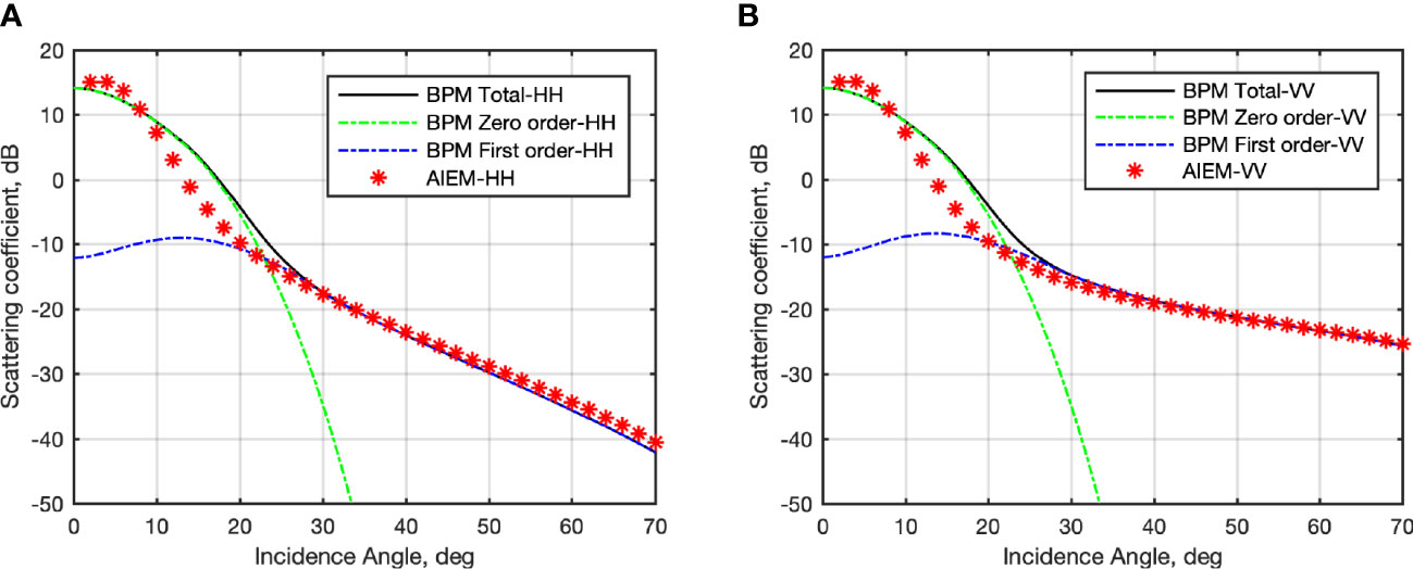
Figure 1 (A) HH- and (B) VV-polarized X-band backscattering coefficients related to a slick-free sea surface predicted by two-scale BPM (continuous black lines) and AIEM (red asterisks) under a wind speed U₁₀=5 ms⁻¹ at variance of incidence angle. The zero (first)-order BPM scattering coefficients are also annotated as dashed green (blue) lines.

2.2. Damping models of sea surface oil films

2.2.1. Marangoni damping model

The well-known “Marangoni effect” can describe the damping of monomolecular slicks such as biogenic films on short wave region of the sea spectrum. In comparison, mineral oil slicks of anthropological origin can form surface-active compounds after weathering and spreading on the sea surface. Moreover, the Marangoni damping with resonance-type characteristics can be observed as well (Alpers and Hühnerfuss, 1988; Gade et al., 2006). The viscous damping of short gravity and capillary sea waves of oil films can be well-modeled according to the Marangoni effect (Lombardini et al., 1989)

$$y_{\text{Mar}}\left(K;\left|E\right|,\theta \right)=\frac{1+X\left(\cos \theta -\sin \theta \right)+XY-Y\sin \theta }{1+2X\left(\cos \theta -\sin \theta \right)+2X^2}$$

with |E| and θ denoting amplitude and phase of the complex dilational coefficient of the surfactant that accounts for its viscoelastic properties. And

$$X=\frac{\left|E\right|K^2}{\sqrt{2{\omega }^3\eta \rho }}$$

$$Y=\frac{\left|E\right|K}{4\omega \eta }$$

where ω is the angular frequency of the sea surface waves while η and ρ are the dynamic viscosity and the density of the sea water, respectively. A surfactant floating on the sea surface affects the full wavenumber omnidirectional sea roughness spectrum while having negligible effect on its directional part (Ermakov et al., 1992; Franceschetti et al., 2002).

The effect of the surfactant on the longer wave part of the roughness spectrum depends on the non-linear wave-wave interactions and on the reduction of the aerodynamic roughness that, at once, is related to the energy input from the wind to the waves, which is represented by the friction velocity. In (Montuori et al., 2016), an empirical relationship between the friction velocity of slick-covered $u_{*,s}$ and slick-free (u_*) sea surface is provided

$$u_{*,s}=\mu ·u_{*}$$

where the reduction factor μ<1 depends both on sea state conditions and the damping properties of the surfactant. Hence, according to (Nunziata et al., 2009; Montuori et al., 2016) the slick-covered sea surface spectrum can be obtained by evaluating the slick-free one at a lower friction velocity ($u_{*,s}$) and, then, damping it by the Marangoni coefficient

$$S_{s,\text{Mar}}\left(K,u_{*,s};\left|E\right|,\theta \right)=\frac{S\left(K,u_{*,s}\right)}{y_{\text{Mar}}\left(K;\left|E\right|,\theta \right)}$$

2.2.2. MLB

The oil films can affect the longer-wave part of the roughness spectrum by nonlinear wave-wave interaction from the longer wave part to the energy sink in the Marangoni dip, together with the reduction of the wind input on the sea surface (Gade et al., 1998a; Gade et al., 1998b; Gade et al., 1998c). Therefore, to include the Marangoni damping and nonlinear interaction, together with the wind input effect on the sea surface spectrum, the action balance equation can be invoked which leads to the damping model of MLB (Alpers and Hühnerfuss, 1989). The latter predicts a damping coefficient that depends on the wind growth rate β , the viscous dissipation term 2Δc_g, with c_g being the group velocity of the sea waves, and the non-linear wave-wave interactions rate α

$$y_{\text{MLB}}\left(K,u_{*,s},y_{\text{Mar}}\right)=\frac{\beta \left(u_{*,s}\right)-2C_g\left(\Delta ·y_{\text{Mar}}\right)+\left(\alpha +\Delta \alpha \right)}{\beta \left(u_{*}\right)-2C_g\Delta +\alpha }$$

According to the MLB, the viscous damping coefficient of the slick-covered sea surface   consists of: a) reducing the wind energy input through a reduced friction velocity that, at once, affects the wind growth rate β(u_*,s); b) enhancing the viscous dissipation coefficient Δ by the Marangoni coefficient (Δ·y_Mar); c) increasing the nonlinear transfer rate by a factor Δ α . Note in this study the wave breaking term in the action balance equation has been ignored since the breaking-wave dissipation is negligible when the wind speeds are less than 10 ms^-1, which is the oil slicks detectable wind condition for SAR (Franceschetti et al., 2002). Therefore, the slick-covered sea surface spectrum can be evaluated by the slick-free one S(K,u_*) damped by the MLB coefficient y_MLB

$$S_{s,\text{MLB}}\left(K,u_{*,s};y_{\text{Mar}}\right)=\frac{S\left(K,u_{*}\right)}{y_{\text{MLB}}\left(K;u_{*,s},y_{\text{Mar}}\right)}$$

From above it can be seen that the process to obtain the slick-covered sea spectrum differs in two aspects: the benchmark slick-free spectrum and the damping coefficient. In 2.2.1, the Marangoni coefficient is combined with the wind-reduced spectrum S(K,u_*,s). While in 2.2.2, the MLB damping coefficient is combined with the non-reduced spectrum S(K,u_*) since includes the wind reduction. To give a better understanding of the two damping coefficients with respect to the kind of surfactants, the damping coefficient (y_Mar and y_MLB ) and the slick-covered full range sea surface spectrum (S_s,Mar and S_s,MLB ) are depicted in Figures 2A, B, respectively. The spectral damping coefficient is depicted for both a biogenic surfactant and a weathered oil slick. The former refers to an oleyl alcohol, which is usually used to simulate a biogenic surfactant (Gade et al., 1998b; Gade et al., 1998a), whose rheological parameters are | E|=0.0255 Nm⁻¹ and θ=−175°, with μ=0.7; while the weathered oil slick calls for rheological parameters that are | E|=0.01 Nm⁻¹ and θ=−175°, with μ=0.575 (Hünerfuss et al., 1989). In Figure 2A, their spectral damping coefficients are depicted with blue and orange lines, respectively. The damping coefficient is modeled using the Marangoni coefficient y_Mar , see continuous lines, and the MLB y_MLB , see dashed lines. Although from a strict theoretical viewpoint the Marangoni damping should be used to describe the damping due to mono-molecular surfactants, Figure 2A is instructive to gain a better understanding of the different behavior of the two damping coefficients. In both cases of mineral oil and biogenic surfactant, the maximum value of y_Mar and y_MLB locations are almost at the same Bragg wavenumber. However, the largest damping is achieved when y_Mar is used and the largest difference among the two models is achieved in the case of biogenic surfactant (blue lines). It is worth noting that, unlike the Marangoni damping model that call for a narrow resonant-like behavior, the MLB leads to a damping that is spread across the wavenumbers affecting in a non-negligible way also longer waves (Alpers and Hühnerfuss, 1989). According to MLB, the depth of the Marangoni dip (corresponding to the maximum Marangoni damping of continuous lines) is reduced because more energy is being transferred from adjacent spectral regions to the dip region by wave-wave interaction. The more is attenuated (by smaller μ ), the stronger damping in the longer-wave region, since more energy in this region is required to sink into the Marangoni dip because of less energy fed from wind input. The range of Bragg wavenumbers that correspond to X-band microwave impinging on the sea surface with an incidence angle that ranges from 20° to 60° is enclosed in the vertical black dotted lines. It can be noted that the damping peak is out of this range for the simulated biogenic surfactant while it lies in this range for the simulated oil slick.

FIGURE 2

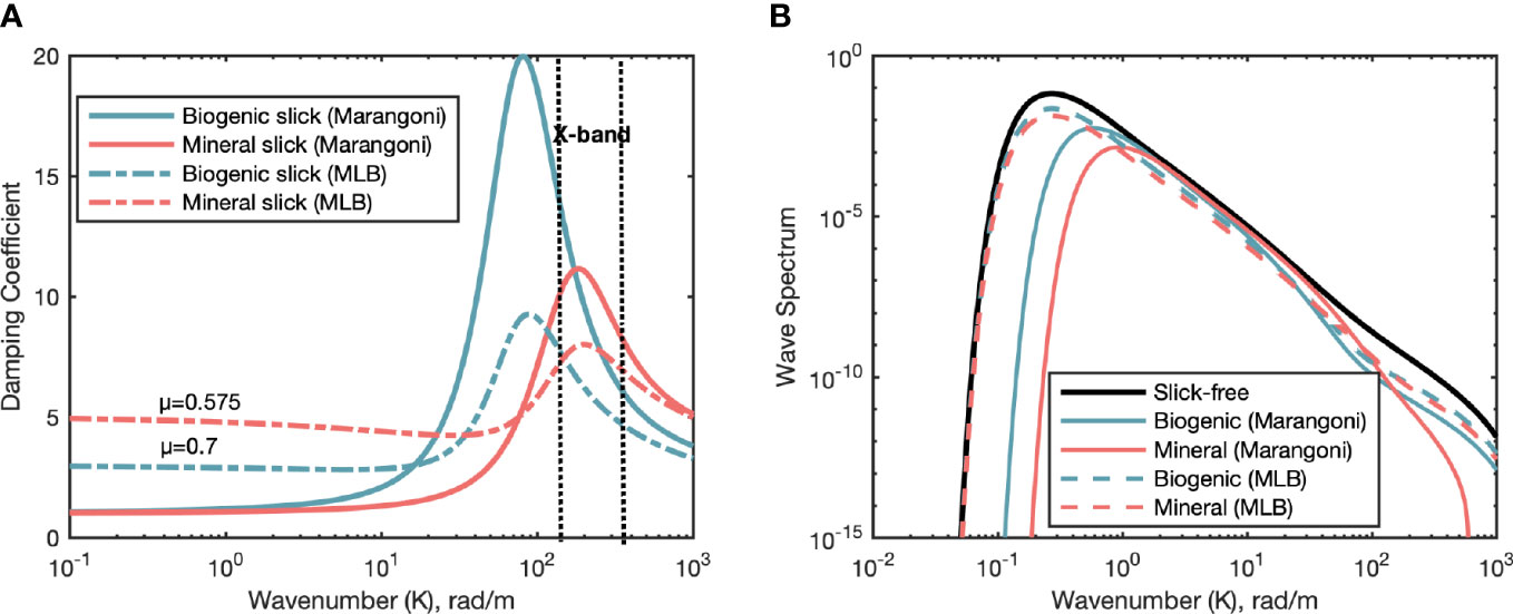
Figure 2 (A) Spectral damping coefficient related to a biogenic film (blue line) and a crude oil (red line) slick evaluated using the Marangoni – continuous line – damping model y_Mar and the MLB dashed – dotted line – damping model y_MLB. Note that the range of X-band Bragg wavenumbers is enclosed by the dotted black vertical lines. (B) Roughness spectrum of a slick-free (black line), biogenic slick-covered (blue line) and crude oil-covered (red line) sea surface. Note that the continuous lines represent S_s,Mar while the dashed lines representing S_s,MLB.

Figure 2B shows the Elfouhaily full-range sea roughness spectrum of slick-free S(K,u_*) (black line) and slick-covered sea surface obtained using the Marangoni coefficient, i.e., S_s,Mar, see continuous lines, and the MLB, i.e., S_s,MLB, see dashed lines, respectively, for both a biogenic surfactant (blue lines) and crude oil (red lines). As expected, the slick-covered spectrum exhibits a departure from the slick-free one in both the short- and the longer-wave parts, which depends on both the kind of surfactant and the considered damping model. When the slick-covered sea surface spectrum is obtained using S_s,Mar, a significant reduction of the energy associated to both the short and longer waves is observed with the largest reduction occurring when the mineral oil is considered. In addition, a significant shift of the peak wavenumber towards shorter waves (related to the reduction of the friction velocity) is observed that is the largest in the case of crude oil. When the slick-covered sea surface spectrum is obtained using S_s,MLB, the peak wavenumber does not change significantly in the slick-covered case and the spectral energy is reduced both at the short- and long-wave parts of the spectrum with the largest reduction occurring, again, in the case of mineral oil.

In conclusion, the MLB provides a more realistic modeling of the surfactant’s effects on the full-range sea surface spectrum.

2.3. Scattering coefficients of slick-covered sea surface and DRs

In this subsection, the scattering coefficient of slick-covered sea surfaces, as well the DR of slicks is predicted using BPM and AIEM and the effect of the surfactant is included using the Marangoni model and the MLB, respectively.

When using the BPM scattering model, the NRCS of the slick-covered sea surface is predicted using 2.1.1 combined with the Marangoni damping on sea spectrum in 2.2.1. The surfactant is supposed to affect a) the zeroth-order term ${\sigma }_{\text{pq},0}^0$ by changing the PDF of the surface slope T_sl and by reducing the roughness on the local tangent plane; b) the first-order term ${\sigma }_{\text{pq},1}^0$ by damping the sea spectrum and shrinking the PDF of the slopes T_sl as described above. In this study, we assumed that the thickness of the surfactant is much smaller than the penetration depth of the incident X-band microwave to consider the surface field function H_pq unaffected by the surfactant (Alpers and Hühnerfuss, 1989; Nunziata et al., 2009). Once the slick-free and the slick-covered NRCSs are available, the DR is predicted as follows

$$D{R}_{\text{BPM}}=\frac{{\sigma }_f^0}{{\sigma }_s^0}=\frac{{\sigma }_{f,0}^0+{\sigma }_{f,1}^0}{{\sigma }_{s,0}^0+{\sigma }_{s,1}^0}$$

where the subscripts f and s denote the slick-free and slick-covered sea surface, respectively.

When using the AIEM scattering model, the NRCS of the slick-covered sea surface is predicted using 2.1.2 combined with the Marangoni model in 2.2.1 and MLB in 2.2.2, respectively. The surfactant affects the sea wave spectrum S(K) and its high-order terms Wⁿ(K), as well as the small-scale rms height σ, which can all be obtained by the oil-covered sea surface spectrum. The DR is predicted as follows

$$D{R}_{\text{AIEM}}=\frac{{\sigma }_f^0}{{\sigma }_s^0}=\text{exp}\left(-2k_{iz}^2\left({\sigma }_f^2-{\sigma }_s^2\right)\right)\frac{\left[{\sum }_{n=1}^{\infty }{\left|I_f\right|}^2\frac{{\left({\sigma }_f^2{W}_f\right)}^n}{n!}\right]}{\left[{\sum }_{n=1}^{\infty }{\left|I_s\right|}^2\frac{{\left({\sigma }_s^2{W}_s\right)}^n}{n!}\right]}$$

where ${\sigma }_f^2$ and ${\sigma }_s^2$ are the square of the rms height for slick-free and slick-covered sea surface, respectively. The polarization-dependent surface field function |I(·)| also depends on the surface rms height; hence they have been explicitly written for both the slick-free |I_f| and the slick-covered case |I_s|.

In Figure 3, the co-polarized DR of slick-covered sea surface are predicted using both BPM and AIEM. Numerical predictions related to the biogenic film and the crude oil slick are depicted using blue and red lines, respectively, while BPM and AIEM scattering models are marked by continuous and dashed lines, respectively. The effect of the surfactant is included in the BPM predictions using the Marangoni damping coefficient in 2.2.1, see continuous lines. In the AIEM predictions the surfactant is accounted for using both Marangoni damping in 2.2.1 and the MLB in 2.2.2 respectively, see dashed lines with and without star marker. The slick-covered sea roughness spectrum is obtained by the slick-free one using the parameters μ suggested in (Gade et al., 1998c; Montuori et al., 2016), i.e.: μ equal to 0.7 and 0.575 for biogenic and mineral oil slicks, respectively. Negative DR values are observed at smaller incidence angles in all model predictions and are due to the enhanced specular reflection arisen from the damping of the small-scale sea waves on the tangent plane.

FIGURE 3

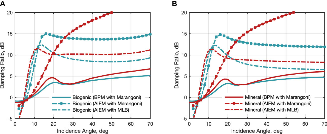
Figure 3 X-band BPM and AIEM predicted DR at HH (A) and VV (B) polarization versus incidence angle. BPM and AIEM predictions are shown in continuous and dashed lines, respectively. The rheological parameters refer to a biogenic slick (blue lines) and a mineral oil slick (red lines). The effect of the surfactant is included using Marangoni damping y_Mar for BPM. While for AIEM, the effect of slicks is included by Marangoni damping y_Mar and MLB damping y_MLB, respectively.

Firstly, to explore the role of scattering model in the prediction of DR, the results by using the same Marangoni damping model combined with BPM (continuous lines) and AIEM (dashed lines with star marker), respectively, are compared. Non-negligible differences apply between BPM and AIEM predictions. By contrasting with Figure 1, one can note that the differences between the NRCSs predicted by the two scattering models under slick-free conditions are emphasized in the slick-covered case, which is due to the different way the effect of the surfactant is included in the two scattering models. For both surfactants, the DR predicted by AIEM are always higher than the BPM one as the incidence angle increases. When the incidence angle is about 20°, the DR difference between BPM and AIEM is about 11 (6) dB for biogenic (mineral oil) slick at both polarizations. As incidence angle increases to about 40°, such the difference becomes more significant for mineral oil with about 13 dB.

Secondly, the effect of various damping models on the predicted DR are explored, which can be obtained by comparing the DR based on AIEM combined with Marangoni damping (dashed lines with star marker) and AIEM damping (dashed line without marker). For incidence angle larger than about 12° (20°), the Marangoni damping always predict higher DR values than MLB for a biogenic (mineral oil) slick. For the incidence angle exceeding 20°, the DR predicted by Marangoni damping is stronger than that by MLB in the case of mineral oil, while their difference stabilized in the range of 4-6 dB in the case of biogenic slick. It is important to note that, as far as for DR plots, even in this case the predictions obtained by augmenting the AIEM with the Marangoni damping coefficient result in a DR that, especially in the mineral oil case (see red dashed lines with star marker), diverge significantly from the predictions resulting from AIEM augmented with MLB and BPM augmented with Marangoni damping coefficient. Such a DR behavior does not seem to be realistic for an oil-covered sea surface.

BPM and AIEM provide consistent (although calling for different NRCS values) predictions for both biogenic- and oil-covered sea surface when the AIEM is augmented with the MLB while the BPM is augmented with Marangoni. According to BPM, the two surfactants are indistinguishable in terms of damping at incidence angles between 20° and 30°. Indeed, they can be distinguished by AIEM in this range of incidence angles, except for angles close to 20°. This analysis points out that the ability to distinguish biogenic surfactants from crude oil through the DR depends significantly on the incidence angle and this dependence is accounted for in a different way by the two scattering models. In addition, the AIEM does not provide reliable DR over oil-covered sea surface when the Marangoni damping is used.

3. Numerical results versus actual measurements

In this section, theoretical predictions are contrasted with actual measurements collected by the X-band TSX satellite mission over sea surface areas where surfactants of known origin are present at low (about 21°) and high (about 40°) incidence angles.

3.1. TSX scene collected at low incidence angle

The TSX SAR scene was acquired on June 8, 2011, at 17:12:05 UTC, during an oil-on-water exercise carried out in the North Sea by the Norwegian Clean Seas Association for Operating Companies. The TSX SAR scene was collected in dual co-polarization Stripmap mode (HH and VV) and an excerpt of the whole HH-polarized 5×5 window speckle-filtered NRCS image is shown in Figure 4A. The exercise consisted of releasing at sea plant, emulsion, and crude oil (from left to right in Figure 4A). Since the exercise was to test the equipment and procedure response to oil spill accidents, the mineral oil releases were subjected to mechanical recovery and dispersion before the SAR acquisitions (Skrunes et al., 2013). Therefore, it can be assumed that the crude oil was subjected to a weathering process at the time of SAR imaging. The wind speed, estimated over the slick-free patches of the SAR scene, is around 4.11 ms^-1 (Li and Lehner, 2013). The NRCS of the slick-free and slick-covered sea surface is predicted according to the two scattering models using SAR, environmental and rheological parameters listed in Table 1, see TSX (A).

FIGURE 4

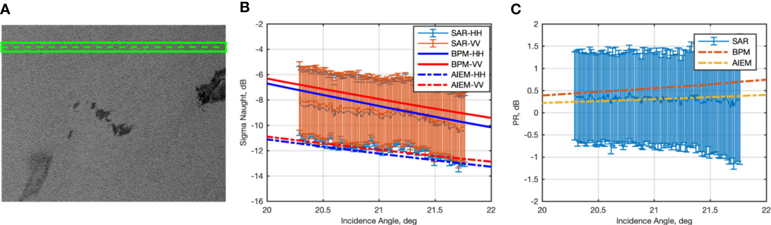
Figure 4 Experiments related to the TSX SAR scene acquired on June 8, 2011, at low incidence angle (about 21°), see Table 1. (A) Excerpt of the HH-polarized speckle-filtered SAR scene. From the leftmost part of the image to the rightmost one, plant, emulsion and crude oil slicks can be observed. The image also includes a ROI, marked in green color, used to analyze the reference sea surface backscattering. (B) Mean and standard deviation values (errorbars) of the HH- and VV-polarized NRCSs measured within the slick-free ROI, together with the NRCSs predicted by BPM and AIEM. (C) Mean and standard deviation values (errorbars) of PR measured within the slick-free ROI contrasted with the one predicted by BPM and AIEM.

TABLE 1

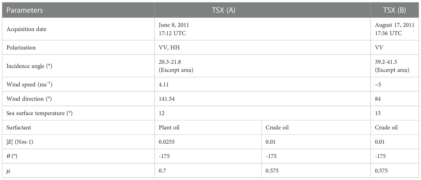
Table 1 SAR, Environmental and Rheological Parameters.

The 200-pixel wide green strip in Figure 4A highlights the region of interest (ROI) of clean sea surface considered to evaluate the statistics (mean with vertical error bars evaluated over each bin consisting of 50 pixels) of the backscattered signal at both VV and HH polarizations, see orange and blue errorbars in Figure 4B, respectively. The NRCS predicted by the two-scale BPM (continuous lines) and AIEM (dashed lines) is also shown in red and blue colors for VV and HH polarization, respectively, using the same parameters of the TSX (III.A) scene listed in Table 1. The BPM scattering model exhibiting a NRCS best fitting the measured one at both polarizations (the mean error is about ±1 dB) in the range of incidence angles spanning 20° to 22°. The AIEM NRCS is always about 3 dB lower than the BPM and the measured one.

The availability of dual-polarimetric TSX SAR measurements suggests investigating the joint behavior of the co-polarized channels using the polarization ratio (PR), i.e., the ratio between the VV- to HH-polarized NRCS. PR is evaluated over the slick-free ROI of Figure 4A and shown (again, as mean and standard deviation values evaluated for each 50-pixel bin) in Figure 4C. The mean value measured for the PR is 0.308 dB. PR is also predicted using both the BPM and the AIEM scattering models and depicted in Figure 4C as red and yellow dashed lines, respectively. The BPM results in a PR that exhibits a behavior steeper than both the AIEM and the measured one with respect to the incidence angle. The mean PR value (0.303 dB) predicted by the AIEM results in very fair agreement with the measured one, while the BPM predicts a mean PR value quite larger than the measured one, i.e., 0.548 dB.

In Figure 4 the low backscatter areas due to the plant and crude oil slicks are analyzed by contrasting measurements with model’s predictions obtained using the two-scale BPM augmented with the Marangoni damping coefficient and the AIEM augmented with the MLB.

3.1.1. Plant oil

In Figure 5A, a close-up view of the plant oil slick area in the TSX image of Figure 4A is shown. The blue and green boxes, consisting of 50×50 pixels each, indicate the ROIs selected to analyze the behavior of the NRCS resulting from the plant oil and the reference slick-free sea surface areas, respectively. They call for approximately the same incidence angle. The mean and standard deviation VV-polarized NRCS values measured for each box are shown in Figure 5C together with BPM (continuous lines) and AIEM (dashed lines) NRCSs predicted for slick-free (blue lines) and biogenic (plant oil) slick-covered sea surface (red lines). A fairly good agreement applies between measured and predicted NRCSs. The two scattering models result in remarkable differences when dealing with the prediction of the NRCS related to the slick-covered sea surface, with the AIEM predicting lower backscattered signals compared to the TSX SAR measurements and BPM predictions. The better performance provided by the BPM scattering model is also confirmed by the DR shown in Figure 5E, where the measured VV-polarized DR is contrasted with the BPM and AIEM predictions. The mean values of the measured DR range approximately between 2 dB and 4 dB with a standard deviation equal to 3.82 dB. The DR predicted by BPM is equal to 2.46 dB at an incidence angle around 20.5°, while a much larger DR value is predicted by AIEM (about 10.37 dB). A similar behavior applies for the HH-polarized NRCSs and DRs, see Figures 5G, I, respectively.

FIGURE 5

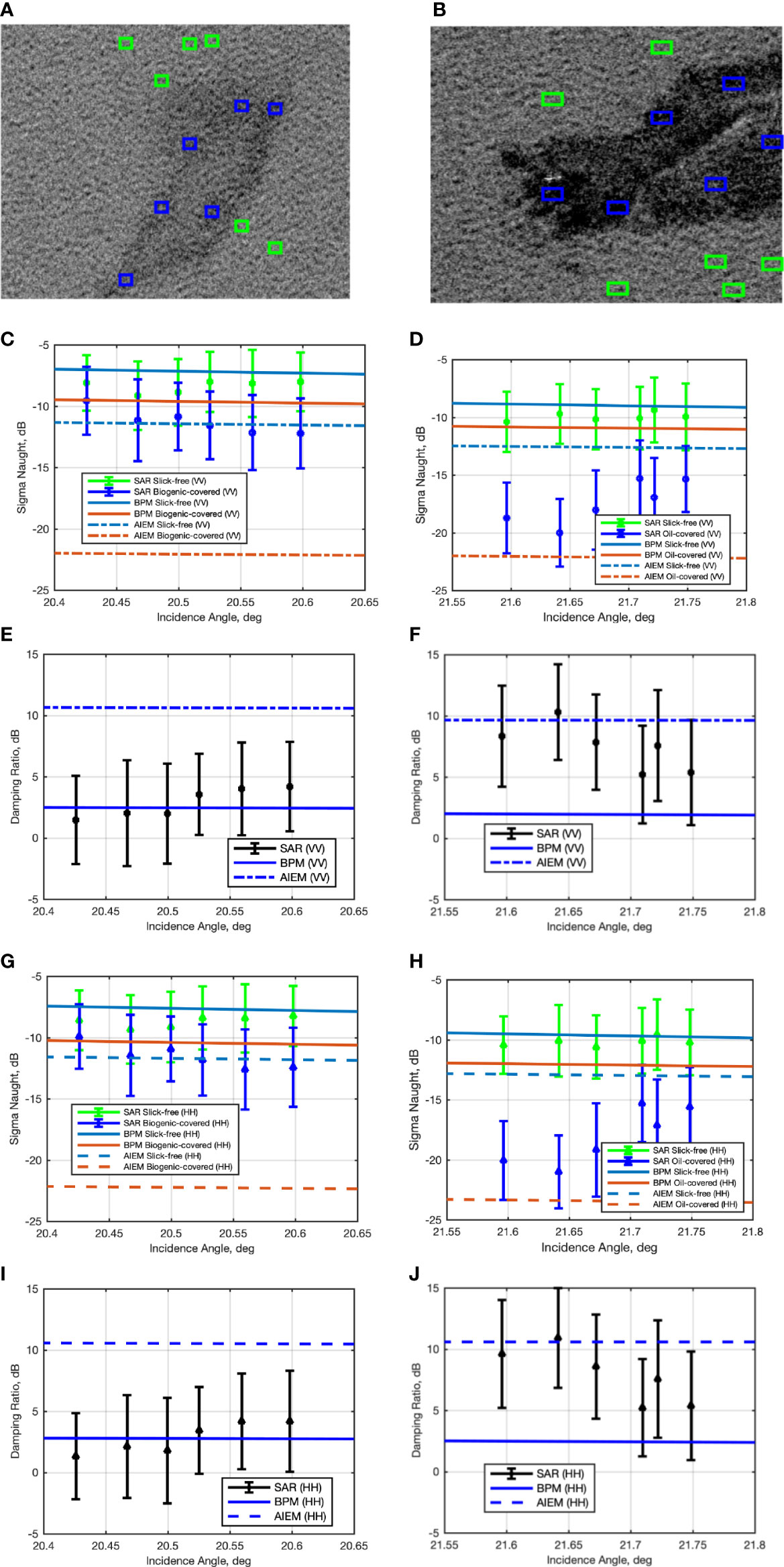
Figure 5 Experiments related to the TSX SAR scene acquired on June 8, 2011, at low incidence angle (about 21°), see Table 1. The first row are excerpts of the TSX SAR scene that includes (A) plant oil and (B) crude oil. The slick-free and slick-covered ROIs selected for quantitative analysis are also annotated in green and blue colors, respectively. The second row are the contrast of VV-polarized NRCS measured within slick-free and slick-covered ROIs with predictied ones in the case of (C) plant oil and (D) crude oil. The third row are the contrast of VV-polarzied DR measured from ROIs with predicted ones in the case of (E) plant oil and (F) crude oil. The forth row (G, H) are the same as (C, D) but for HH-polarized NRCS. And the fifth row (I, J) are the same as (E, F) but for HH-polarized DR.

3.1.2. Mineral oil

In Figure 5B, a close-up view of the crude oil slick area in the TSX image of Figure 4A is shown. The brighter spot represents the ship involved in the oil-on-water exercise. In Figure 5D, the VV-polarized NRCS values predicted by BPM and AIEM are contrasted with the NRCS measured within slick-free and oil-covered ROIs highlighted in Figure 5B. Again, both BPM and AIEM result in a predicted slick-free NRCS that agrees with the measured one. Remarkable differences between the two models apply in the oil-covered case where the AIEM results in a predicted NRCS that best fits the measured one. This is also confirmed by the VV-polarized DR predicted by AIEM that provides the best agreement with the measured one. The latter calls for a mean value that lies in the range 5 dB – 10 dB which, as expected, is larger than that of the plant oil slick. A remarkable standard deviation value applies, i.e., about 4.12 dB, which is larger than the plant oil slick one. This larger variability could be related to the chemical dispersion and the weathering that affected the crude oil from the releasing to the SAR imaging time. Similar comments apply when analyzing the HH-polarized NRCS and DR, see Figures 5H, J, respectively.

It must be noted that, by jointly discussing Figures 5E, F, the difference between the VV-polarized DR values predicted for plant and mineral oil slick is about 0.4 (0.8) dB for BPM (AIEM). This small difference is mainly due to the incidence angle as shown in Figure 4C. It is worth noting that, when dealing with low backscatter areas in SAR imagery, a key issue to be considered is the reliability of the measured NRCS with respect to the noise equivalent sigma zero (NESZ), i.e., the signal-to-noise-ratio. To be reliable, the NRCS measured over a low backscatter area should be larger than the NESZ. In the TSX case, the NESZ lies between -19 dB and -26 dB depending on the imaging mode and incidence angle, with an average value of -21 dB (Eineder et al., 2008). According to (Montuori et al., 2016), the received signal can be considered uncorrupted by noise if it is at least 3 dB larger than NESZ. In this data set, Figure 4B, Figure 5C show that the NRCS measured over slick-free and plant oil slick-covered area is more than 3 dB larger than the NESZ, which is about -19 dB. This is not always the case for the NRCS measured over the oil-covered ROIs, see Figures 5D, H, which may lie at the level or even below the NESZ.

3.2. TSX scene collected at high incidence angle

The TSX SAR scene was acquired on August 17, at 17:36 UTC, in the North Sea, see Table 1 (B). The speckle-filtered VV-polarized NRCS image is shown in Figure 6A where a crude oil slick released during the Gannet Alpha oil rig accident occurred on August 14, 2011, is visible as an elongated patch darker than the sea background. The surface wind speed is around 5 ms^-1 (Nunziata et al., 2019). The three ROIs considered for quantitative analysis, i.e., one over clean sea surface (green) and two over the oil slick – since it exhibits an elongated shape, they are extracted closer to and farther away the oil rig site (red and orange boxes, respectively). The mean and standard deviation NRCS values related to the slick-free ROI are depicted in Figure 6B where the NRCSs predicted by BPM and AIEM are also annotated as continuous and dashed blue lines, respectively. The mean and standard deviation NRCS values measured over the slick-free ROI are equal to about -20.9 dB and ±1.5 dB, respectively. As far as for the previous experiment, both models predict NRCS values that agree with the measured ones. The difference between the two models’ predictions is about 0.5 dB, which is consistent with the theoretical results shown in Figure 1. In Figure 6C the mean and standard deviation values of the measured DR (evaluated for each 50-pixel bin) is contrasted with BPM and AIEM predicted ones for the ROI closer to (red markers) and farther away (orange markers) the oil rig. Note that the elongated shape of the slick makes difficult selecting oil pixels. Hence, to limit the mixing between sea and oil pixels along the azimuth direction, we focused on measured DR values whose standard deviation is lower than ±2.5 dB. The AIEM predicts a DR of about 7.12 dB that results in a fairly good agreement with the TSX SAR measurements, while the BPM underestimates significantly the DR (about 4.6 dB).

FIGURE 6

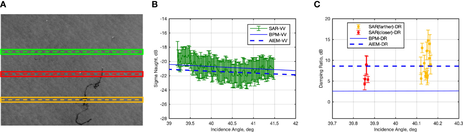
Figure 6 Experiments related to the TSX SAR scene acquired on August 17, 2011, at high incidence angle (about 40°), see Table 1 (A) Excerpt of the VV-polarized speckle-filtered SAR scene. The slick-free ROI (green box) and the two oil slick-covered ROIs (red and orange boxes) used for quantitative analysis are also annotated. (B) The VV-polarized NRCS measured over the slick-free ROI is contrasted with the BPM and AIEM predicted one. (C) The measured DR related to red and orange oil-covered ROIs contrasted with BMP and AIEM predictions.

The ROI closer to the oil rig site (see red markers in Figure 6C), calls for a measured DR whose mean values span the range from 4 dB to 8 dB. The ROI farther away from the oil rig site (see orange markers in Figure 6C) calls for mean DR values spanning a larger range, i.e., from 5 dB to 15 dB. This witnesses that, compared to the fresher oil spilled closer to the oil rig, as far as one moves away from the rig site a stronger weathering applies to the oil that exhibits more complex and heterogeneous characteristics. One should also note that the thickness of mineral oil may vary within the oil slick generating areas with varying characteristics affecting the backscattered signals (Espeseth et al., 2020).

4. Conclusions

In this study, the two-scale BPM and AIEM scattering models augmented with Marangoni damping coefficient and the MLB are used to predict the NRCS related to slick-free and slick-covered sea surface. From numerical analysis, the scattering model and the damping model both play a non-negligible role in predicting the DR of scattering from sea surface slicks. The predicted values are contrasted with actual TSX SAR measurements collected at low (about 21°) and high (about 40°) incidence angles over slicks of known origin. The main outcomes can be summarized as follows.

When dealing with slick-free sea surface, the two-scale BPM and AIEM result in predicted NRCS values at both polarizations that exhibit non-negligible differences up to an incidence angle of about 40°. Those differences are negligible (less than 1 dB) at larger incidence angles. The NRCS predicted by BPM results in the best agreement with the measured one at low incidence angles. The AIEM results in a PR that best fits actual measurements.

When dealing with slick-covered sea surfaces, the backscattered signals from TSX measurements are utilized to analyze the damping behaviors of plant oil (biogenic) and mineral oil slicks, while the mineral oil slicks generally cause stronger damping on backscattering coefficients at X-band. AIEM and BPM combined with various damping models are used to predict the NRCS and DR. The two scattering models result in significantly different predictions according to the slick type (biogenic or mineral oil) and the considered damping model. In the case of plant oil slicks, the DR predicted by BPM combined with Marangoni damping model results in the best agreement with the DR measured from actual TSX SAR imagery. In the case of mineral oil slicks, the AIEM results in the best predictions at both low and high incidence angles when the MLB damping model is used.

Data availability statement

The original contributions presented in the study are included in the article/supplementary material. Further inquiries can be directed to the corresponding author.

Author contributions

TM performed the experiment, data analysis and drafted the manuscript. FN contributed to the conception of the study, data analysis, and wrote the manuscript. AB helped in the data acquisition and manuscript preparation. XY contributed significantly to analysis with constructive discussions. MM revised the manuscript critically for important intellectual content. All authors contributed to the article and approved the submitted version.

Funding

This study is partly supported by the National Key R&D Program of China (2021YFB3901300), by the ESA-NRSCC Dragon-5 cooperation project (ID 57979), by the China Scholarship Council and by the ASI under the APPLICAVEMARS project (ASI contract n. 2021-4-U.0) within the framework of the call DC-UOT-2019-017.

Acknowledgments

The authors would thank the DLR for providing the TSX SAR data under the framework of the project ID OCE3201 entitled “TerraSAR-X SAR data to monitor hazards related to extreme weather conditions and oil pollution”.

Conflict of interest

The authors declare that the research was conducted in the absence of any commercial or financial relationships that could be construed as a potential conflict of interest.

Publisher’s note

All claims expressed in this article are solely those of the authors and do not necessarily represent those of their affiliated organizations, or those of the publisher, the editors and the reviewers. Any product that may be evaluated in this article, or claim that may be made by its manufacturer, is not guaranteed or endorsed by the publisher.

References

Alpers W., Holt B., Zeng K. (2017). Oil spill detection by imaging radars: Challenges and pitfalls. Remote Sens. Environ. 201, 133–147. doi: 10.1016/j.rse.2017.09.002

CrossRef Full Text | Google Scholar

Alpers W., Hühnerfuss H. (1988). Radar signatures of oil films floating on the sea surface and the marangoni effect. J. Geophys. Res. Oceans 93, 3642–3648. doi: 10.1029/JC093iC04p03642

CrossRef Full Text | Google Scholar

Alpers W., Hühnerfuss H. (1989). The damping of ocean waves by surface films: A new look at an old problem. J. Geophys. Res. Oceans 94, 6251–6265. doi: 10.1029/JC094iC05p06251

CrossRef Full Text | Google Scholar

Boisot O., Angelliaume S., Guérin C.-A. (2018). “Physical modeling of oil at Sea: Application for microwave Co-polarized radar imagery,” in IGARSS 2018-2018 IEEE International Geoscience and Remote Sensing Symposium. 45–48 (Valencia, Spain: IEEE).

Google Scholar

Brekke C., Solberg A. H. (2005). Oil spill detection by satellite remote sensing. Remote Sens. Environ. 95, 1–13. doi: 10.1016/j.rse.2004.11.015

CrossRef Full Text | Google Scholar

Chen G., Li Y., Sun G., Zhang Y. (2017). Application of deep networks to oil spill detection using polarimetric synthetic aperture radar images. Appl. Sci. 7, 968. doi: 10.3390/app7100968

CrossRef Full Text | Google Scholar

Chen K.-S., Wu T.-D., Tsang L., Li Q., Shi J., Fung A. K. (2003). Emission of rough surfaces calculated by the integral equation method with comparison to three-dimensional moment method simulations. IEEE Trans. Geosci. Remote Sens. 41, 90–101. doi: 10.1109/TGRS.2002.807587

CrossRef Full Text | Google Scholar

De Laurentiis L., Jones C. E., Holt B., Schiavon G., Del Frate F. (2020). Deep learning for mineral and biogenic oil slick classification with airborne synthetic aperture radar data. IEEE Trans. Geosci. Remote Sens. 59, 8455–8469. doi: 10.1109/TGRS.2020.3034722

CrossRef Full Text | Google Scholar

Du Y., Yang X., Chen K.-S., Ma W., Li Z. (2017). An improved spectrum model for sea surface radar backscattering at l-band. Remote Sens. 9, 776. doi: 10.3390/rs9080776

CrossRef Full Text | Google Scholar

Eineder M., Fritz T., Mittermayer J., Roth A., Boerner E., Breit H. (2008). TerraSAR-X ground segment, basic product specification document, Cluster applied remote sensing (caf) oberpfaffenhofen. (Berlin, Heidelberg: Springer)

Google Scholar

Ermakov S., Salashin S., Panchenko A. (1992). Film slicks on the sea surface and some mechanisms of their formation. Dyn. Atmos. Oceans 16, 279–304. doi: 10.1016/0377-0265(92)90010-Q

CrossRef Full Text | Google Scholar

Espeseth M. M., Jones C. E., Holt B., Brekke C., Skrunes S. (2020). Oil-spill-response-oriented information products derived from a rapid-repeat time series of SAR images. IEEE J. Sel. Topics Appl. Earth Obs. Remote Sens. 13, 3448–3461. doi: 10.1109/JSTARS.2020.3003686

CrossRef Full Text | Google Scholar

Fingas M., Brown C. E. (2018). A review of oil spill remote sensing. Sensors 18, 91. doi: 10.3390/s18010091

CrossRef Full Text | Google Scholar

Franceschetti G., Iodice A., Riccio D., Ruello G., Siviero R. (2002). SAR raw signal simulation of oil slicks in ocean environments. IEEE Trans. Geosci. Remote Sens. 40, 1935–1949. doi: 10.1109/TGRS.2002.803798

CrossRef Full Text | Google Scholar

Fung A. K. (1994). Microwave scattering and emission models and their applications (Norwood, MA: Artech House).

Google Scholar

Fung A. K. (2015). Backscattering from multiscale rough surfaces with application to wind scatterometry (MA, USA, Artech House: Norwood).

Google Scholar

Gade M., Alpers W., Hühnerfuss H., Lange P. A. (1998a). Wind wave tank measurements of wave damping and radar cross sections in the presence of monomolecular surface films. J. Geophys. Res. Oceans 103, 3167–3178. doi: 10.1029/97JC01578

CrossRef Full Text | Google Scholar

Gade M., Alpers W., Hühnerfuss H., Masuko H., Kobayashi T. (1998b). Imaging of biogenic and anthropogenic ocean surface films by the multifrequency/multipolarization SIR-C/X-SAR. J. Geophys. Res. Oceans 103, 18851–18866. doi: 10.1029/97JC01915

CrossRef Full Text | Google Scholar

Gade M., Alpers W., Hühnerfuss H., Wismann V. R., Lange P. A. (1998c). On the reduction of the radar backscatter by oceanic surface films: Scatterometer measurements and their theoretical interpretation. Remote Sens. Environ. 66, 52–70. doi: 10.1016/S0034-4257(98)00034-0

CrossRef Full Text | Google Scholar

Gade M., Hühnerfuss H., Korenowski G. (2006). Marine surface films.

Google Scholar

Garcia-Pineda O., Macdonald I. R., Li X., Jackson C. R., Pichel W. G. (2013). Oil spill mapping and measurement in the gulf of Mexico with textural classifier neural network algorithm (TCNNA). IEEE J. Sel. Topics Appl. Earth Obs. Remote Sens. 6, 2517–2525. doi: 10.1109/JSTARS.2013.2244061

CrossRef Full Text | Google Scholar

Guissard A., Sobieski P., Baufays C. (1992). A unified approach to bistatic scattering for active and passive remote sensing of rough ocean surfaces. Trends Geophys. Res. 1, 43–68.

Google Scholar

Guo H., Wu D., An J. (2017). Discrimination of oil slicks and lookalikes in polarimetric SAR images using CNN. Sensors 17, 1837. doi: 10.3390/s17081837

PubMed Abstract | CrossRef Full Text | Google Scholar

Hühnerfuss H., Alpers W., Garrett W. D., Lange P. A., Stolte S. (1983). Attenuation of capillary and gravity waves at sea by monomolecular organic surface films. J. Geophys. Res. Oceans 88, 9809–9816. doi: 10.1029/JC088iC14p09809

CrossRef Full Text | Google Scholar

Hünerfuss H., Alpers W., Witte F. (1989). Layers of different thicknesses in mineral oil spills detected by grey level textures of real aperture radar images. Int. J. Remote Sens. 10, 1093–1099. doi: 10.1080/01431168908903947

CrossRef Full Text | Google Scholar

Ivonin D., Brekke C., Skrunes S., Ivanov A., Kozhelupova N. (2020). Mineral oil slicks identification using dual Co-polarized radarsat-2 and TerraSAR-X SAR imagery. Remote Sens. 12, 1061. doi: 10.3390/rs12071061

CrossRef Full Text | Google Scholar

Latini D., Del Frate F., Jones C. E. (2016). Multi-frequency and polarimetric quantitative analysis of the gulf of Mexico oil spill event comparing different SAR systems. Remote Sens. Environ. 183, 26–42. doi: 10.1016/j.rse.2016.05.014

CrossRef Full Text | Google Scholar

Lemaire D., Sobieski P., Craeye C., Guissard A. (2002). Two-scale models for rough surface scattering: Comparison between the boundary perturbation method and the integral equation method. Radio Sci. 37, 1–16. doi: 10.1029/1999RS002311

CrossRef Full Text | Google Scholar

Li Y., Huang W., Lyu X., Liu S., Zhao Z., Ren P. (2022). An adversarial learning approach to forecasted wind field correction with an application to oil spill drift prediction. Int. J. Appl. Earth. Obs. 112, 102924. doi: 10.1016/j.jag.2022.102924

CrossRef Full Text | Google Scholar

Li X.-M., Lehner S. (2013). Algorithm for sea surface wind retrieval from TerraSAR-X and TanDEM-X data. IEEE Trans. Geosci. Remote Sens. 52, 2928–2939. doi: 10.1109/TGRS.2013.2267780

CrossRef Full Text | Google Scholar

Li G., Li Y., Liu B., Hou Y., Fan J. (2018). Analysis of scattering properties of continuous slow-release slicks on the sea surface based on polarimetric synthetic aperture radar. ISPRS Int. J. Geo-Inf. 7, 237. doi: 10.3390/IJGI070237

CrossRef Full Text | Google Scholar

Li Y., Lyu X., Frery A. C., Ren P. (2021). Oil spill detection with multiscale conditional adversarial networks with small-data training. Remote Sens. 13, 2378. doi: 10.3390/rs13122378

CrossRef Full Text | Google Scholar

Lombardini P. P., Fiscella B., Trivero P., Cappa C., Garrett W. (1989). Modulation of the spectra of short gravity waves by sea surface films: slick detection and characterization with a microwave probe. J. Atmos. Ocean. Technol. 6, 882–890. doi: 10.1175/1520-0426(1989)006“0882:MOTSOS”2.0.CO;2

CrossRef Full Text | Google Scholar

Meng T., Chen K.-S., Yang X., Nunziata F., Xie D., Buono A. (2021a). Simulation and analysis of bistatic radar scattering from oil-covered Sea surface. IEEE Trans. Geosci. Remote Sens. 60, 1–15. doi: 10.1109/TGRS.2021.3137654

CrossRef Full Text | Google Scholar

Meng T., Yang X., Chen K.-S., Nunziata F., Xie D., Buono A. (2021b). Radar backscattering over Sea surface oil emulsions: Simulation and observation. IEEE Trans. Geosci. Remote Sens. 60, 1–14. doi: 10.1109/TGRS.2021.3073369

CrossRef Full Text | Google Scholar

Montuori A., Nunziata F., Migliaccio M., Sobieski P. (2016). X-Band two-scale sea surface scattering model to predict the contrast due to an oil slick. IEEE J. Sel. Topics Appl. Earth Obs. Remote Sens. 9, 4970–4978. doi: 10.1109/JSTARS.2016.2605151

CrossRef Full Text | Google Scholar

Nunziata F., De Macedo C. R., Buono A., Velotto D., Migliaccio M. (2019). On the analysis of a time series of X–band TerraSAR–X SAR imagery over oil seepages. Int. J. Remote Sens. 40, 3623–3646. doi: 10.1080/01431161.2018.1547933

CrossRef Full Text | Google Scholar

Nunziata F., Sobieski P., Migliaccio M. (2009). The two-scale BPM scattering model for sea biogenic slicks contrast. IEEE Trans. Geosci. Remote Sens. 47, 1949–1956. doi: 10.1109/TGRS.2009.2013135

CrossRef Full Text | Google Scholar

Pinel N., Bourlier C., Sergievskaya I. (2013). Two-dimensional radar backscattering modeling of oil slicks at sea based on the model of local balance: Validation of two asymptotic techniques for thick films. IEEE Trans. Geosci. Remote Sens. 52, 2326–2338. doi: 10.1109/TGRS.2013.2259498

CrossRef Full Text | Google Scholar

Pinel N., Déchamps N., Bourlier C. (2008). Modeling of the bistatic electromagnetic scattering from sea surfaces covered in oil for microwave applications. IEEE Trans. Geosci. Remote Sens. 46, 385–392. doi: 10.1109/TGRS.2007.902412

CrossRef Full Text | Google Scholar

Plant W. J. (1986). A two-scale model of short wind-generated waves and scatterometry. J. Geophys. Res. Oceans 91, 10735–10749. doi: 10.1029/JC091iC09p10735

CrossRef Full Text | Google Scholar

Rice S. O. (1951). Reflection of electromagnetic waves from slightly rough surfaces. Commun. Pur. Appl. Math. 4, 351–378. doi: 10.1002/cpa.3160040206

CrossRef Full Text | Google Scholar

Skrunes S., Brekke C., Eltoft T. (2013). Characterization of marine surface slicks by radarsat-2 multipolarization features. IEEE Trans. Geosci. Remote Sens. 52, 5302–5319. doi: 10.1109/TGRS.2013.2287916

CrossRef Full Text | Google Scholar

Solberg A. H. S. (2012). Remote sensing of ocean oil-spill pollution. Proc. IEEE 100, 2931–2945. doi: 10.1109/JPROC.2012.2196250

CrossRef Full Text | Google Scholar

Valenzuela G. R. (1978). Theories for the interaction of electromagnetic and oceanic waves–a review. Bound.-Layer Meteor. 13, 61–85. doi: 10.1007/BF00913863

CrossRef Full Text | Google Scholar

Voronovich A. (1994). Small-slope approximation for electromagnetic wave scattering at a rough interface of two dielectric half-spaces. Waves Random Media 4, 337. doi: 10.1088/0959-7174/4/3/008

CrossRef Full Text | Google Scholar

Wismann V., Gade M., Alpers W., Huhnerfuss H. (1998). Radar signatures of marine mineral oil spills measured by an airborne multi-frequency radar. Int. J. Remote Sens. 19, 3607–3623. doi: 10.1080/014311698213849

CrossRef Full Text | Google Scholar

Xie D., Chen K.-S., Yang X. (2019a). Effect of bispectrum on radar backscattering from non-Gaussian sea surface. IEEE J. Sel. Topics Appl. Earth Obs. Remote Sens. 12, 4367–4378. doi: 10.1109/JSTARS.2019.2946934

CrossRef Full Text | Google Scholar

Xie D., Chen K.-S., Yang X. (2019b). Effects of wind wave spectra on radar backscatter from sea surface at different microwave bands: A numerical study. IEEE Trans. Geosci. Remote Sens. 57, 6325–6334. doi: 10.1109/TGRS.2019.2905558

CrossRef Full Text | Google Scholar

Xie D., Chen K.-S., Zeng J. (2019c). The frequency selective effect of radar backscattering from multiscale sea surface. Remote Sens. 11, 160. doi: 10.3390/rs11020160

CrossRef Full Text | Google Scholar

Yang C.-S., Park S.-M., Oh Y., Ouchi K. (2013). An analysis of the radar backscatter fromoil-covered sea surfaces usingmomentmethod andMonte-Carlo simulation: preliminary results. Acta Oceanol. Sin. 32, 59–67. doi: 10.1007/s13131-013-0267-7

CrossRef Full Text | Google Scholar

Zhang J., Feng H., Luo Q., Li Y., Wei J., Li J. (2020). Oil spill detection in quad-polarimetric SAR images using an advanced convolutional neural network based on SuperPixel model. Remote Sens. 12, 944. doi: 10.3390/rs12060944

CrossRef Full Text | Google Scholar