Variance-based sensitivity analysis of oil spill predictions in the Red Sea region

To support accidental spill rapid response efforts, oil spill simulations may generally need to account for uncertainties concerning the nature and properties of the spill, which compound those inherent in model parameterizations. A full detailed account of these sources of uncertainty would however require prohibitive resources needed to sample a large dimensional space. In this work, a variance-based sensitivity analysis is conducted to explore the possibility of restricting a priori the set of uncertain parameters, at least in the context of realistic simulations of oil spills in the Red Sea region spanning a two-week period following the oil release. The evolution of the spill is described using the simulation capabilities of Modelo Hidrodinâmico, driven by high-resolution metocean fields of the Red Sea (RS) was adopted to simulate accidental oil spills in the RS. Eight spill scenarios are considered in the analysis, which are carefully selected to account for the diversity of metocean conditions in the region. Polynomial chaos expansions are employed to propagate parametric uncertainties and efficiently estimate variance-based sensitivities. Attention is focused on integral quantities characterizing the transport, deformation, evaporation and dispersion of the spill. The analysis indicates that variability in these quantities may be suitably captured by restricting the set of uncertain inputs parameters, namely the wind coefficient, interfacial tension, API gravity, and viscosity. Thus, forecast variability and confidence intervals may be reasonably estimated in the corresponding four-dimensional input space.

1 Introduction

Oil spill forecasting is extremely important in preventive planning and post-oil spill management. Forecasting requires a solid understanding of the prevailing oil spill dynamics, typically gained through a high-fidelity model that captures the transport of oil and its physio-chemical transformations, referred to as weathering (Zodiatis et al., 2021). Weathering processes include evaporation, dispersion into the water column, emulsification, and spreading (Lehr et al., 2002), all of which depend on the local atmospheric and oceanic conditions (Oudot et al., 1998; Transportation Research Board and National Research Council, 2003).

Most oil spill models employ a Lagrangian particle tracking algorithm (van Sebille et al., 2018), for example, MEDSLIK II (De Dominicis et al., 2013b; De Dominicis et al., 2013a) and Modelo Hidrodinâmico [MOHID; http://www.mohid.com/; e.g., (Neves, 2013)]. These models rely on ocean currents and atmospheric conditions and incorporate parametrizations to account for subgrid-scale processes. When subgrid parametrizations are adequately calibrated, and the spill conditions are faithfully described, the spill models effectively forecast the evolution of oil spills (Hodges et al., 2015; Barker et al., 2020).

Many sources of uncertainty arise when modeling oil spills in oceanic flows, including uncertainties in metocean conditions, forcing and model parameters (Xu et al., 2012; Iskandarani et al., 2016a; Iskandarani et al., 2016b). In a rapid response scenario, these uncertainties may be further compounded by a lack of knowledge of the nature of the spill oil and/or its physical properties. Addressing all these sources of uncertainty simultaneously is computationally prohibitive, and it is consequently advantageous to explore whether it is possible to ignore some of the uncertain inputs characterizing oil properties and model parametrizations, without significantly deteriorating our ability to quantify the variability of the predictions. This is the central question that we explore in the present study, namely in in the framework of a limited, two-week long, simulations of oil spills in the RS region, which is at risk of oil spill events due to the significant number of oil tankers traversing the basin (Alkhshall and Westcott, 2019; Kleinhaus et al., 2020; Kostianaia et al., 2020; Dong et al., 2022). Our approach to this question is based on considering a limited set of scenarios that captures the diversity of met-ocean conditions in the region, and to conduct a systematic analysis of the impact of parametric uncertainties for this set of scenarios. This offers to enable us to identify a priori a small set of key parameters that dominate the variability of the predictions, and to ignore the others. Of course, such parameter space would lead to substantial gains, as one would be able to determine confidence bounds at a reduced computational burden.

Despite its fundamental and practical relevance, little work has been done in the literature to quantify the sensitivity of oil spill forecasts on the oil and model parameters. Previous studies dealt with a qualitative assessment of the model output’s sensitivity to input parameters (Lopes, 2016), whereas others were relied on a quantitative assessment based on local sensitivities (Mateus and Franz, 2015); namely on relative model output variation for variations in the input, or based on a normalized error approach (Oliveira et al., 2020). Whereas local sensitivity methods provide simple and effective means to analyze forecast variability, their application to reduce the space of random parameters may be prone to errors, especially when mixed effects are important. To overcome such potential drawbacks, global sensitivity analysis (GSA) considers the full space of uncertain inputs (Adetula and Bokov, 2011). Generally, GSA implementations are categorized as variance-based (Sobol, 1993; Homma and Saltelli, 1996; Sobol, 2001) or entropy-based (Lüdtke et al., 2008; Martorell et al., 2008). In both cases, the analysis considers the variability of an entire set of parameters, simultaneously and in the entire range of their priors (Sudret, 2008). Additionally, it yields total sensitivity indices that account for both direct and mixed interactions, providing robust means for identifying which parameters can be effectively neglected.

In the present study, we rely on Sobol’s total sensitivity indices to analyze the variability of the model forecast (Homma and Saltelli, 1996). These provide a variance-based estimate of the sensitivity of selected model outputs due to uncertainties in individual parameters. This approach relies on an orthogonal hierarchical decomposition of the variance to produce robust estimates that can be readily leveraged for the purpose of parameter space reduction. It has in fact shown to be an effective tool in a different areas, including ocean modeling applications (Srinivasan et al., 2010; Alexanderian et al., 2012; Winokur et al., 2013; Goncalves et al., 2016; Wang et al., 2016) among others [e.g. (Navarro Jimenez et al., 2016; Huan et al., 2018; KC et al., 2021)].

The paper is structured as follows. Section 2 outlines the scope of the study, providing a brief description of the oil spill model, the selection of metocean conditions and spill scenarios, and of a screening study used to define a reasonable set of key uncertain inputs. As described in Section 3, a polynomial chaos (PC) approach is adopted to construct surrogates of selected quantities of interest (QoIs), quantify variances, and efficiently estimate Sobol indices (Crestaux et al., 2009). Simulation results are presented and analyzed in Section 4. Concluding remarks are provided in Section 5.

2 Data and methodology

This section describes the metocean data of the RS, which were used to drive the oil spill model. Specifically, Sections 2.1.1 and 2.1.2 describe the metocean fields and their spatial and seasonal variabilities, respectively. The selected oil spill scenarios are outlined in Section 2.1.3. Section 2.2 presents the oil spill model employed to simulate the evolution of an oil spill. The QoIs describing the evolution of the oil slick geometry, transport, and weathering processes are reported in Section 2.3. Finally, Section 2.4 discusses the screening process conducted to select uncertain parameters with the strongest influence on the released oil.

2.1 Red Sea and metocean dataset

2.1.1 Metocean numerical modeling

The RS hosts one of the world’s most diverse tropical marine habitats (Chiffings et al., 1995), including the third-largest coral reef system in the world (Carvalho et al., 2019). Fisheries, water desalination plants, and several mega-projects, such as NEOM, lie along its coast (Hoteit et al., 2021). The RS seasonally and regionally experiences widely varying metocean conditions (Yao et al., 2014a; Yao et al., 2014b). Accordingly, the RS is divided into three regions: the northern, central, and southern RS, each with unique but interweaving circulation patterns (Carvalho et al., 2019).

Further described below, the RS metocean fields we employ in the present work were extracted from high-resolution simulations (Langodan et al., 2017; Viswanadhapalli et al., 2017; Dasari et al., 2019; Hoteit et al., 2021), which provide reliable descriptions of the oceanic and atmospheric circulation of the RS region. The zonal and meridional winds were extracted from an in-house 5-km regional atmospheric reanalysis specifically generated for the RS region using the weather research forecasting (WRF) model. The WRF initial and boundary conditions were obtained from the European Centre for Medium-Range Weather Forecasts Reanalysis Interim (Dee et al., 2011) data. The WRF downscaling simulations were performed using the consecutive daily reinitialization method over 36-h periods (Viswanadhapalli et al., 2017; Dasari et al., 2019). The wave conditions in the RS were reconstructed using the WAVEWATCH III model forced with the mentioned high-resolution WRF reanalysis winds on a 1-km grid (Langodan et al., 2017).

The three-dimensional (3D) ocean currents were simulated using the Massachusetts Institute of Technology general circulation model (MITgcm) (Marshall et al., 1997) implemented at an approximately 1-km grid resolution with 50 nonuniform vertical layers. The model was forced with the mentioned WRF atmospheric reanalysis fields and open boundary in the Gulf of Aden, which were obtained from the Copernicus Marine and Environment Monitoring Service global ocean reanalysis fields, on a 6-h and 24-h basis, respectively (https://marine.copernicus.eu/). Readers are referred to (Hoteit et al., 2021) for a detailed description and validation of the WRF, WAVEWATCH III, and MIT general circulation model fields.

2.1.2 Variability of metocean condition in the Red Sea

The high mountain ranges on both sides of the RS force the wind to blow along its main axis (Langodan et al., 2014). During summer, from April to October, a northwesterly wind blows along the whole length of the sea (Langodan et al., 2014). In winter, the same northerly wind dominates over the northern part of the basin, and southeasterly winds associated with the northeasterly winds of the monsoon in the Indian Ocean prevail over the southern RS. The coexistence of northerly and southerly winds creates a convergence zone at the center of the RS (Langodan et al., 2017). The larger and smaller valleys across the bordering mountain ridge lead to typical local winds relevant for characterizing local wind regimes, for example, the wind passing through the Tokar Gap along the Sudan coast in summer and the westward blowing jets along the northeastern coast of the RS in winter (Langodan et al., 2014; Viswanadhapalli et al., 2017).

The wave variability in the RS is naturally associated with the dominant regional wind regimes (Langodan et al., 2014). During summer, the northwesterly winds prevailing over the whole RS generate mean wave heights of 1 to 1.5 m in the north (Langodan et al., 2014). In winter, the monsoon-associated winds generate mean wave heights of approximately 2 m in the southern RS, leading to a convergence zone in the central part when they meet the waves from the north (Langodan et al., 2017).

The mean surface circulation in the southern RS is largely moderated by the wind regime, which reverses between seasons. During winter, when the southeasterly winds prevail, the surface inflow from the Gulf of Aden intensifies as a western boundary current in the southern basin and switches to an eastern boundary current north of 24°N (Yao et al., 2014a). In summer, the dominant northeasterly winds push the surface outflow from the RS into the Gulf of Aden (Yao et al., 2014b). In the central and northern RS regions, circulation is primarily characterized by multiple mesoscale eddies that tend to become more energetic during winter following the development of intense baroclinic instabilities (Zhan et al., 2019), except for some strong semi-permanent wind-driven gyres that occur in summer (Zhan et al., 2019).

2.1.3 Oil spill scenarios

Pertaining to our main objective of exploring whether the space of uncertain parameters can be restricted a priori, eight scenarios were selected corresponding to four release locations and two release times. Note that the selection was guided by a desire to cover a wide range of relevant environmental conditions, particularly to build confidence in any a priori reduction. Of course, the surrogate models constructed for the selected metocean conditions are not expected to be representative of other ocean states. However, quantitative variability and sensitivity trends established for a sufficiently diverse set of scenarios are also expected to hold in more general conditions.

The selected release locations are depicted in Figure 1, which also displays some of the surface fields at the first of January and August. Specifically, the selected release locations include one spot in the northern RS, two in the central RS, and one in the southern RS. Spills initiated on the first of January and another on the first of August were selected to assess the influence of various metocean circulation conditions on the oil spill dynamics. As can be seen from the illustrations provided in Figure 1, the selected metocean conditions reflect distinct ocean states. Specifically, the spill conditions considered may be initiated at the center or periphery of coherent ocean eddies, or in situations characterized by turbulent small scale eddies. Similarly, the release may occur in conditions involving large or small wave heights, strong or weak surface winds, and high or low sea surface temperature. The resulting diversity of release conditions considered thus helps build confidence that any a priori reduction in the space of parameters that results from the analysis will also hold generally hold for the Red Sea region.

FIGURE 1

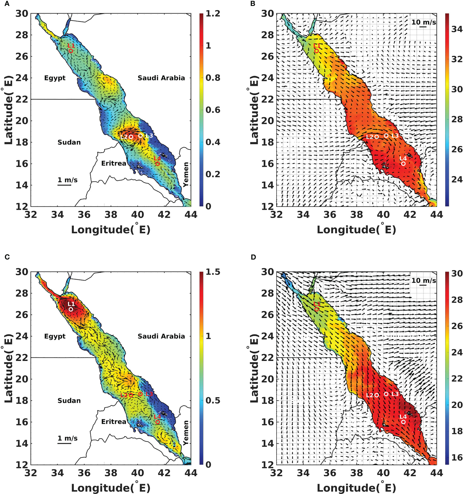
Figure 1 Left column (A, C): composite illustration of significant wave height (m) and surface currents (m/s); right column (B, D): composite illustration of sea surface temperature (°C) and surface winds (m/s). The top (A, B) and bottom (C, D) rows illustrate the average fields for the first of August and January of 2016, respectively. The release locations L1–4 are also depicted.

The release locations in the central RS cover the center and periphery of a long-lived eddy that experiences predictable movement during summer but more complex chaotic motion during winter. The release location in the northern RS is prone to strong wind effects that generate strong waves during summer. The circulation in the north is also dominated by mesoscale eddies that intensify in energy in winter. Finally, release Location 4 is selected to examine the influence of the metocean conditions in the south, which are tightly related to the Indian Monsoon, and the effect of the inflow current from the Arabian Sea. In the analysis below, Location 1 is the release location in the northern RS, and Location 2 is the release location at the center of the eddyin the central RS. Location 3 is the release location at the periphery of the eddy in the central RS, and Location 4 is the release location in the southern RS.

2.2 Oil spill model

Modelo Hidrodinâmico’s (MOHID) Lagrangian and oil models are components of the MOHID Water Modeling System (http://www.mohid.com/) adopted to simulate the results of oil spills. In addition, MOHID is an open-source, 3D water modeling system developed by the Marine and Environmental Technology Research Center at the Technical University of Lisbon (Leitao et al., 2013). Together, the models simulate oil trajectories while accounting for the physico-chemical transformations of the oil. The Lagrangian model is responsible for transporting individual particles, accounting for the effects of diffusion, buoyancy, Stokes drift, windage, linear degradation, and land interaction, such as beaching. Moreover, the oil model simulates the effects of the weathering processes, including dispersion, evaporation, sedimentation, spread, dissolution, and emulsification. The MOHID Lagrangian and oil spill models are driven by the outputs of the high-resolution RS metocean fields discussed in Section 2.1.1 (Hoteit et al., 2021).

A Cartesian grid uniformly spaced in the horizontal directions, longitude and latitude, and nonuniformly spaced in vertical layers was adopted for the current applications. The grid covers the entire RS between longitudes 32°E and 46°E and latitudes 10°N and 30°N up to a depth of approximately 2,746 m. The longitudinal and latitudinal axes are divided into 1,401 and 2,001 equally spaced nodes, respectively, corresponding to a grid resolution of approximately 1 km on both axes. The metocean input fields, including the daily averaged 3D ocean currents, hourly winds, wave height, and period, are specified on the same horizontal and vertical grids. The time step of the oil model was set to 60 s to properly describe the weathering processes, which vary over very short time scales, and the results were reported at 15-min intervals. The time step of the Lagrangian model to transport the individual particles was set to 3,600 s, and the results were reported at 3-h intervals. For each release scenario, 5,000 oil particles were released from the release point, where the Lagrangian and oil models advected and simulated weathering under metocean conditions. The performance and accuracy of MOHID for oil spill modeling have already been demonstrated in many previous studies and ocean basins [e.g., (Li, 2017) and (Mittal et al., 2021)].

2.3 Quantities of interest

This section discusses the QoIs used to characterize the transport and geometry of the oil slick and selected weathering processes. We explored several ways to characterize the shape and deformation of the surface oil. Specifically, we examined the second-order particle moments centered on the centroid of the realized oil slick or nominal oil slick. A more detailed description of these integral quantities is provided. We also investigated distance measures between the realized and reference spills, such as the Hausdorff distance and the ${\ell }_2$ distance between concentration or binary maps, attributing a value of 1 to the grid cells with surface oil and 0 for no oil. For brevity, we focus on the central and nominal second-order particle moments.

The general $(p,q)$-moment is defined according to the following:

$\begin{array}{ll}{M}_{p,q}=\sum _i{x}_{1,(i)}^p{x}_{2,(i)}^q,& (1)\end{array}$

where the sum is performed over all surface particles with nonzero mass. The transportation of the oil slick is characterized by the location of its centroid or first moment, estimated as follows:

$\begin{array}{ll}\overline{x}=\frac{M_{1,0}}{M_{0,0}}=\frac{{\sum }_i{x}_{1,(i)}^1{x}_{2,(i)}^0}{N},& (2)\end{array}$

$\begin{array}{ll}\overline{y}=\frac{M_{0,1}}{M_{0,0}}=\frac{{\sum }_i{x}_{1,(i)}^0{x}_{2,(i)}^1}{N},& (3)\end{array}$

where $N$ is the total number of particles with a nonzero mass. These equations yield the longitude and latitude of the centroid (C Lon and C Lat, respectively) that describe the mean geometric location of the oil slick.

To characterize the shape of the surface slick, we rely on the second-order central particle moments (Rocha et al., 2002). Specifically, we extracted the particle covariances expressed by the following:

$\begin{array}{ll}a=\frac{M_{2,0}}{M_{0,0}}-{\overline{x}}^2=\frac{{\sum }_i{x}_{1,(i)}^2{x}_{2,(i)}^0}{N}-{\overline{x}}^2,& (4)\end{array}$

$\begin{array}{ll}b=\frac{M_{1,1}}{M_{0,0}}-\overline{x} \overline{y}=\frac{{\sum }_i{x}_{1,(i)}^1{x}_{2,(i)}^1}{N}-\overline{x} \overline{y},& (5)\end{array}$

$\begin{array}{ll}c=\frac{M_{0,2}}{M_{0,0}}-{\overline{y}}^2=\frac{{\sum }_i{x}_{1,(i)}^0{x}_{2,(i)}^2}{N}-{\overline{y}}^2 ,& (6)\end{array}$

which enables characterizing an elliptical region associated with the surface slick.

In addition, the second-order moments relative to the nominal oil slick centroid are introduced, leading to covariances denoted by $\widehat{a}$, $\widehat{b}$, and $\widehat{c}$, which are obtained by replacing $\overline{x}$ and $\overline{y}$ in the system above with ${\overline{x}}_o$ and ${\overline{y}}_o$, respectively, which are the longitude and latitude of the centroid of the nominal oil slick. The nominal scenario corresponds to the deterministic prediction obtained using the average value of the input parameters. Whereas $a$, $b$, and $c$ characterize the shape of individual oil slicks, $\widehat{a}$, $\widehat{b}$, and $\widehat{c}$ characterize the region where spilled oil is likely to be present.

Finally, we rely on the fraction of mass evaporated (FME) and the fraction of mass dispersed (FMD) to characterize weathering processes. In addition, the QoIs are summarized and briefly described in Table 1. Figure S1 illustrates an example for release at Location 3 during summer. The distribution of surface oil particles and the ellipse characterized using the first and second particle moments are presented.

TABLE 1

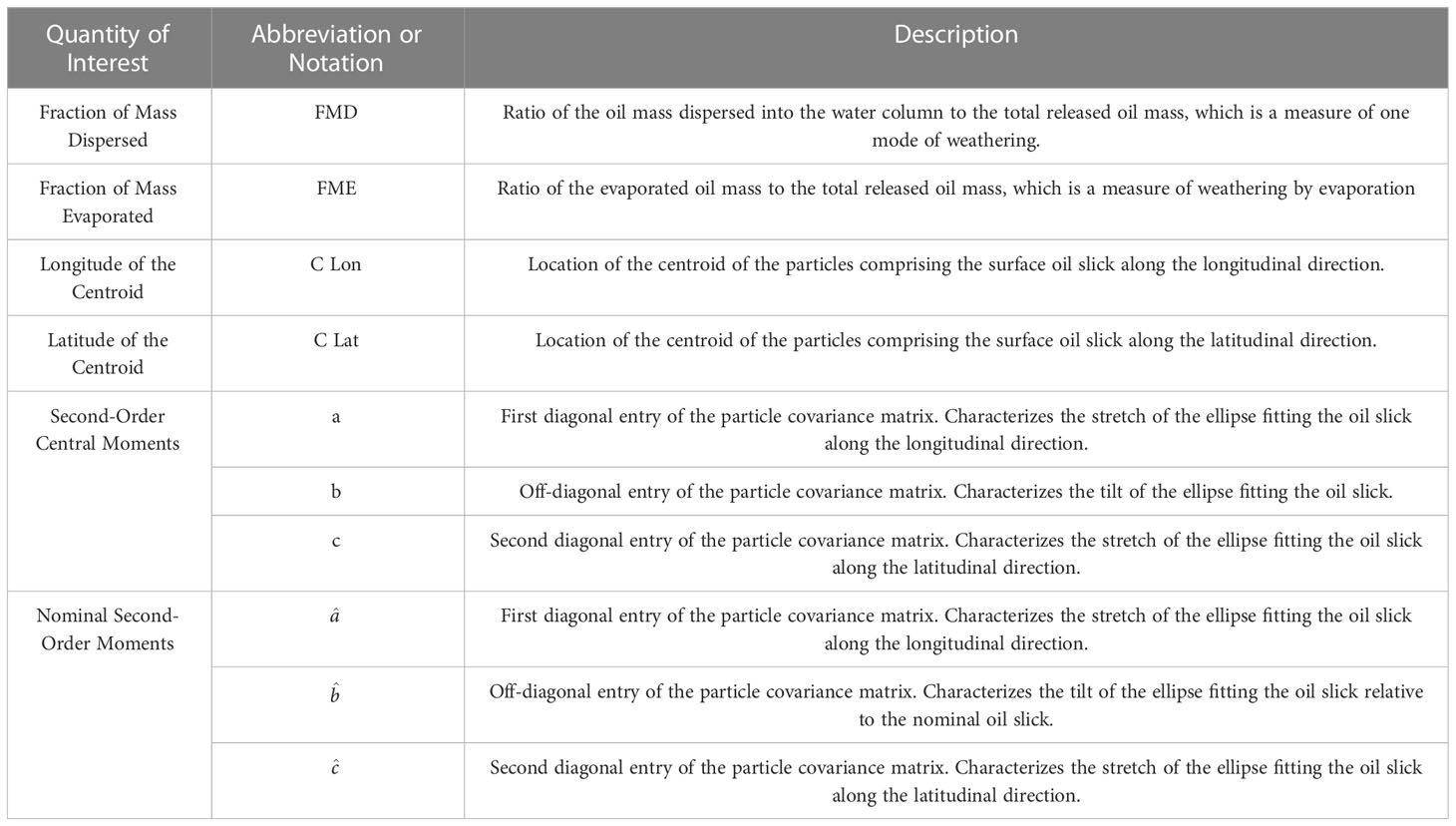
Table 1 Quantities of interest and their associated abbreviations or notation and descriptions.

2.4 Uncertain input parameters

The evolution of simulated ocean oil spills is governed by several parameters related to the physical oil properties and model parametrizations. An initial screening was conducted by varying a single parameter at a time and observing its effects on the oil spill evolution. The parameters examined in this preliminary screening study are summarized in Table 2. These include Fay’s spread, the empirical thickness gradient (ETG) spread coefficient, the emulsification coefficient, the water uptake parameter (WUP), wind coefficient (WC), the American Petroleum Institute gravity (API), pour point temperature, asphaltene content, dynamic viscosity, and interfacial tension (IFT).

TABLE 2

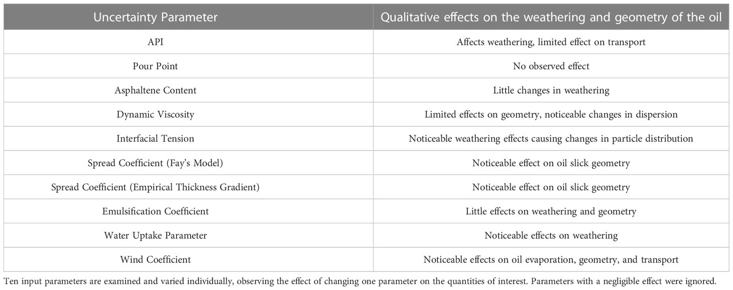
Table 2 Screening study to shortlist uncertainty parameters of the oil spill model, keeping those of interest to construct surrogate models.

The effects of each parameter in Table 2 on the QoIs were analyzed, focusing on the resulting total (peak-to-peak) variability. The results indicated that the parameters with the strongest influence on the QoIs consisted of oil properties (API, viscosity, IFT) and model parameterizations (wind coefficient, ETG, and water uptake parameter). These six parameters were consequently retained in the GSA.

Table 3 reports the retained uncertainty parameters and the variability ranges extracted from the literature. The choice of prior distributions has a significant impact on the results of PC models, and it is generally considered advantageous to rely on distributions that reflect the prior state of knowledge (Thacker et al., 2015; Wang et al., 2016). Because information on the joint or marginal distributions of the parameters in Table 3 was not available, however, the analysis treated the individual parameters as uncorrelated and imposed an uninformative prior for each of the parameters considered. Because the parameters had bounded ranges, a uniform prior was consequently selected.

TABLE 3

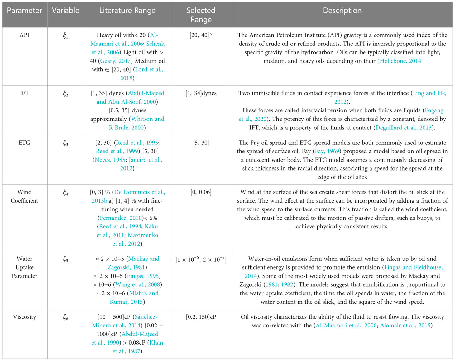
Table 3 Uncertainty parameters with variable notation, value range considered in the referenced literature, range selected for constructing the surrogate model, and a brief description of the uncertain input.

3 Polynomial chaos methodology

This section discusses the PC methodology (Wiener, 1938; Ghanem and Spanos, 1991; Le Maître and Knio, 2010) to construct functional representations of QoIs in terms of uncertain inputs. A nonintrusive regularized regression technique outlined in Section 3.1 is applied for this purpose. A brief discussion is provided in Section 3.2 concerning how surrogates are exploited to estimate the global variance-based sensitivities of QoIs to uncertain inputs.

3.1 Polynomial chaos expansions

In the PC approach (Knio and Le Maître, 2006; Le Maître and Knio, 2010; Sraj et al., 2017), uncertain inputs are parametrized in terms of a vector of independent canonical random variables, $\xi$. The dependence of a generic QoI, $X$, on the uncertain inputs is approximated by a truncated series of the following form:

$\begin{array}{ll}X(\xi )\approx {\displaystyle \sum _{k=0}^P{c}_k{\text{Ψ}}_k(\xi ),}& (7)\end{array}$

where ${\text{Ψ}}_k$denotes the orthogonal basis function defined over the probability space associated with $\xi$, $c_k$ represents the expansion coefficients to be determined, and $P+1$ indicates the size of the approximation basis.

In light of the discussion in Section 2, $d$ uncertain input parameters are parametrized using $d$ independent canonical random variables uniformly distributed over ${[-1,1]}^d$. Thus, the random vector $\xi =\left\{{\xi }_1,\dots ,{\xi }_d\right\}$ has components whose physical ranges coincide with those of the associated model parameters in Table 3. The basis functions ($\text{Ψ}$) are the multidimensional Legendre polynomials in the random vector $\xi$. A generic input parameter is expressed as $p_i(\xi )={\mu }_i+{\sigma }_i{\xi }_i$ for $i=1,\dots ,d$. In this formulation, ${\mu }_i=\frac{1}{2}(a_i+b_i)$ denotes the nominal value of $p_i$, ${\sigma }_i=\frac{1}{2}(b_i-a_i)$ represents half its range, and $a_i$ and $b_i$ represent the lower and upper bounds of the physical range of $p_i$, respectively. We adopted a total order truncation technique so that the truncated basis size is as follows:

$$P+1=\frac{(d+p)!}{d!p!},$$

where $p$ denotes the maximal polynomial degree of the truncated expansion.

PC expansions are generally classified as global or local depending on the span of the stochastic space covered by the model (Najm, 2009). In the present study we focus on global PC models, rely on a so-called non-intrusive methodology to determine the PC coefficients (Eldred, 2009; Lüthen et al., 2021). This indicates that the coefficients are determined using the outputs deterministic forward model runs, performed at suitable realizations of the uncertain inputs. An overview of different methods to generate PC surrogate models could be found in (Najm, 2009; Hadigol and Doostan, 2018; Lüthen et al., 2021).

In preliminary work, we investigated constructing surrogates using projection-based methods based on Gauss and Gauss–Kronrod–Paterson quadratures (Laurie, 1997) and regularized regression following the least absolute shrinkage and selection operator (LASSO) algorithm (Tibshirani, 1996; Roth, 2004; Ranstam and Cook, 2018). The study suggested that surrogates obtained using the LASSO regression yielded lower reconstruction errors than the pseudospectral projection counterparts. The large errors in the projection-based surrogates were due to the noisy particle approximations of the QoIs. Because the regression approach is robust to noisy estimates, it was adopted to construct the surrogates and support the GSA. Note that several open source libraries such as UQ toolkit (Debusschere et al., 2017) and UQLab (Marelli and Sudret, 2014) provide implementations of projection and regression methods that can be readily used to efficiently build PC surrogates.

In the LASSO regression, the coefficients are obtained by minimizing the sum of residuals between the observed variable and PC expansion prediction, and an ${\ell }_1$ regularization term is introduced to prevent overfitting. The functional to be minimized is as follows:

$\begin{array}{ll}R(c_k)=\left(\frac{1}{2N}\sum _{i=1}^N{\left(y_i-{\displaystyle \sum _{k=0}^P{c}_k{\text{Ψ}}_k({\xi }^{(i)})}\right)}^2+\lambda \sum _{k=1}^P\left|c_k\right|\right),& (8)\end{array}$

where $N$ represents the number of observations, $y_i$ indicates the QoI at observation $i$, ${\xi }^{(i)}$ denotes the i^th observation point, and $\lambda$ represents a positive regularization constant to be determined. The LASSO algorithm is applied with 10-fold cross-validation to estimate the model error (Obuchi and Kabashima, 2016). The optimal value of $\lambda$ yields the smallest cross-validation mean squared error. Once determined, the corresponding coefficient vector is adopted to define the PC surrogate.

3.2 Global sensitivity analysis

The Sobol indices estimate the influence of the input uncertainties on the variability in the model output by evaluating the ratio of the conditional variances to the total variance of the output. Using the same notation as in the work by (Crestaux et al., 2009), the sensitivity index corresponding to the index set $i\subset D\equiv \left\{1,\dots ,d\right\}$ are defined as:

$\begin{array}{ll}{S}_i\equiv \frac{V_i(X)}{V(X)}=\frac{E[X^2({\xi }_i)]}{V(X)}& (9)\end{array}$

whereas the corresponding total sensitivity index is defined according to:

$\begin{array}{ll}{T}_i\equiv \frac{E_{{\xi }_{\sim i}}[V_{{\xi }_i}(X|{\xi }_{\sim i})]}{V(X)},& (10)\end{array}$

where $X$ is a generic QoI, $d$ is the total number of dimensions, $E$ and $V$ denote the expectation and variance operators, respectively, and $\sim i$ represents the complement of the subset $i$ in $D$.

The Sobol sensitivity indices could be estimated efficiently using the PC expansion by exploiting the orthogonality of the PC basis (Sobol, 1993; Homma and Saltelli, 1996; Sobol, 2001; Sudret, 2008; Crestaux et al., 2009; Le Maître and Knio, 2010; Alexanderian et al., 2012). The Sobol indices are given by:

$\begin{array}{ll}{S}_i\approx \frac{{\sum }_{k\in S_i}{c}_k^2|\left|{\Psi }_k\right|{|}_2^2}{{\sum }_{k\ge 1}{c}_k^2|\left|{\Psi }_k\right|{|}_2^2},& (11)\end{array}$

where $S_i=\left\{k\right|{\text{Ψ}}_k\text{ has degree }0\text{ in all }{\xi }_j\text{ with }j\notin i\}$. Similarly, the total sensitivity index corresponding to the singleton $\left\{i\right\}$can be readily obtained using:

$\begin{array}{ll}{T}_i\approx \frac{{\sum }_{k\in T_i}{c}_k^2|\left|{\Psi }_k\right|{|}_2^2}{{\sum }_{k\ge 1}{c}_k^2|\left|{\Psi }_k\right|{|}_2^2},& (12)\end{array}$

where $T_i=\left\{k|{\text{Ψ}}_k\text{ has degree }\rangle 0\text{ in }{\xi }_i\right\}$. Note that the Sobol indices $S_i$ account for the so-called direct contributions of the uncertain parameters ${\xi }_i$, and that $T_i$ accounts for both the direct contributions of the uncertain variable ${\xi }_i$ as well as its mixed interactions with the remaining variables. In particular, it can readily be seen that a small $T_i$ justifies neglecting ${\xi }_i$ and according restricting the uncertain input space.

4 Results and discussion

4.1 Assessment of the surrogate model

The $N=600$ realizations (${\xi }^{(i)}$) of the random germ ($\xi$) were generated using a Latin hypercube sampling algorithm to generate PC surrogates. The same realizations of the germ were used for each of the eight considered scenarios, and MOHID was applied to simulate the evolution of the corresponding spills. As discussed in the previous section, PC surrogates of the selected QoIs were determined by solving the LASSO regression problem based on the simulation outputs. This section analyzes the performance of the PC surrogates by computing the associated time-dependent normalized ${\ell }_2$errors:

$\begin{array}{ll}{E}_2(t)\frac{\sqrt{\frac{1}{N}{\displaystyle {\sum }_{i=1}^N{(f({\xi }^{(i)},t)-\widehat{f}({\xi }^{(i)},t))}^2}}}{\left(\underset{\xi }{\max }f(\xi ,t)-\underset{\xi }{\min }f(i,t)\right)} ,& (13)\end{array}$

where $f$ denotes a generic QoI obtained from the MOHID simulation, $\widehat{f}$ is the corresponding QoI approximated by the PC surrogate, and the maximum and minimum function values are defined over all realizations and simulation times in the order indicated. PC surrogate models ranging from first to sixth total order expansions were constructed, and their reconstruction errors were evaluated. The fifth-order PC model was selected because it offered the best compromise between suitable reconstruction errors and computational time. Consequently, the study presents results obtained using a degree five total order truncation.

An illustration of the performance of the PC surrogate is provided in Figure 2A, which depicts the evolution of C Lon and C Lat for a randomly selected realization of $\xi$. The results for release Location 1 are used, and curves are generated for winter and summer release scenarios using the MOHID outputs and corresponding PC surrogates. The PC representation errors are depicted in Figure 2B. As expected, errors corresponding to C Lon and C Lat increase with time for both release seasons. Nonetheless, the $E_2$ metric remains below 6% throughout the simulation period, indicating that the PC representation remains suitable for estimating sensitivities over the entire simulation time, which is reflected in the close alignment between the curves in Figure 2A.

FIGURE 2

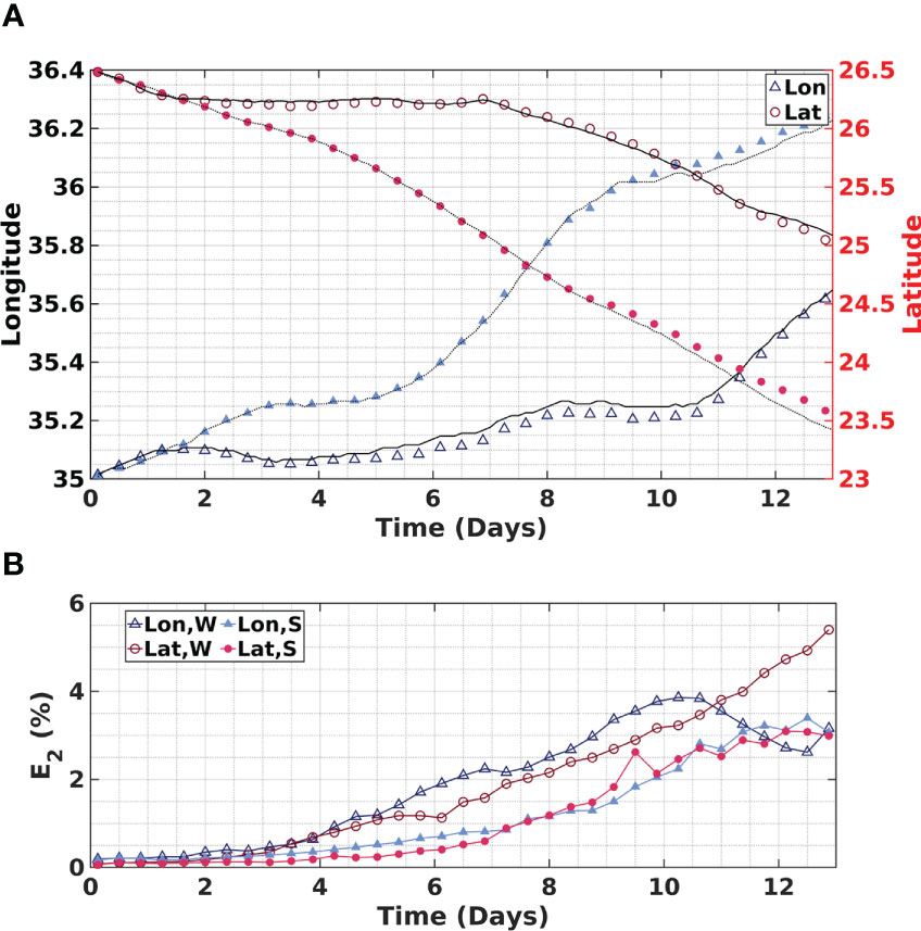
Figure 2 Illustration of the (A) evolution of C Lon (triangles) and its Lat (circles) for the winter (W, hollow) and summer (S, filled) releases as predicted by the surrogate model and compared to the corresponding MOHID output (black) for winter (solid) and summer (dashed) releases; (B) evolution of $E_2$ in time for C Lon and C Lat for summer and winter releases.

We also analyzed the maximum values over time of $E_2$ for all considered QoIs and all release scenarios; see Supplementary Table S1. Overall, the results exhibit small error values and alignment between the surrogate and the MOHID predictions for the various realizations, indicating that the PC surrogate suitably represents the functional dependence of the QoIs on uncertain inputs.

4.2 Spill motion and deformation

Figures 3A, B illustrate the evolution of the standard deviation of C Lon and C Lat, respectively. Curves are generated for all eight considered scenarios. The results indicate that C Lon and C Lat generally experience substantial variability, with values of the standard deviation exceeding $\mathrm{0.25o}$ in all scenarios. In addition, C Lat generally exhibits greater variability during the winter scenarios, attributed to the more chaotic nature of the RS flow field during the selected winter events. A more chaotic flow leads to higher variability (Zhan et al., 2016).

FIGURE 3

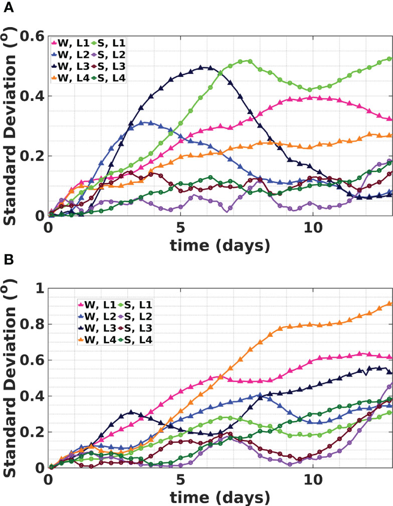
Figure 3 Evolution of the standard deviation of the (A) C Lon and (B) C Lat of the ellipse that fits the oil particles. Evolution curves are presented for summer (S, circles) and winter (W, triangles) and release Locations 1–4.

The figures also demonstrate that the standard deviation of C Lat is greater than that of C Lon, which may be attributed to the topography of the RS basin with a greater extent along the latitude. The evolution of the standard deviation is generally nonmonotonic because of the stretching and folding of the oil slick by the ocean eddies. This nonmonotonic behavior has important implications for analyzing sensitivities, as discussed below. Finally, the figures indicate strong variability across release scenarios for C Lon and C Lat, which indicates that different metocean conditions along the RS basin strongly affect the motion of the spilled oil and significantly affect the evolution of parametric uncertainties. These findings may be readily appreciated by contrasting the mean displacements and their variabilities across the eight considered scenarios. The present observations also underscore the importance of using accurate wind information in oil spill modeling (Keramea et al., 2021).

Figure 4 depicts the particle distributions corresponding to four randomly selected realizations of the parameters. The distributions are plotted two weeks after the initial release. Simulations corresponding to a summer release scenario originating at Location 2 are used for this purpose. The distributions reveal that for two out of the four selected realizations of $\xi$, C Lat is around 18.25°N (frames b and c), whereas for the other two realizations of C Lat is around 17.5°N (frames a and d). The illustrations correspond to samples at the modes of C Lat for the summer release scenario with an initial release from Location 2. The particle distributions also illustrate the variability resulting from using different inputs with the same metocean conditions, see also Figure S2, which depicts the evolution of the PDFs of C Lon and C Lat revealing multimodal behavior. This highlights the importance of properly selecting key model parameters and physical oil properties and accounting for residual uncertainties.

FIGURE 4

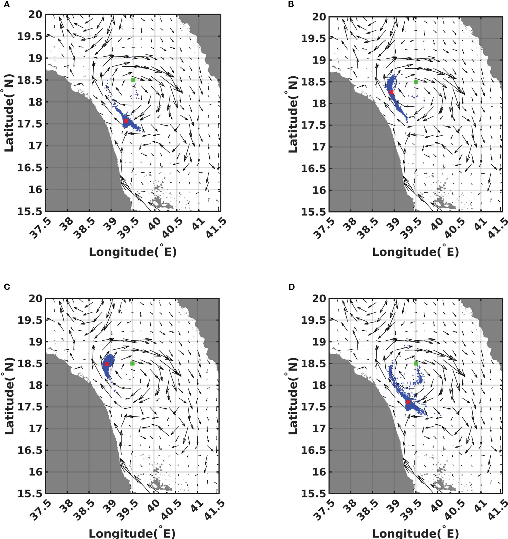
Figure 4 Particle distributions at the last simulation time step (14 days from release) for four realizations of the random germ $\xi$. The distributions are plotted individually and presented in frames (A–D). All simulations correspond to a release occurring during summer from release Location 2. Each frame presents the release source location (green square), oil particles (blue dots), and their center of gravity(red cross). Particles are distributed differently for various combinations of uncertainty parameters. Specifically, for some realizations, the center of gravity is located at a similar latitude as the initial release (frames B, C), whereas for others, the center of gravity is located noticeably southward of the initial release (frames A, D).

Figures 5A, B display the evolution of the total sensitivity indices for C Lon and C Lat for all release locations. The curves are depicted for the summer release scenarios. The results for the winter scenarios were similar and, thus, omitted. The results indicate that the wind coefficient has the greatest influence on the location of the oil spill centroid. Around Day 9, the sensitivity of C Lon and C Lat with respect to the viscosity briefly rises, but this behavior is insignificant because the variances drop to small values around that time. Similar behavior also occurs with IFT and approximately 10 days after the initial release of oil. These results imply that, among the investigated parameters, the wind coefficient is the dominant input parameter affecting the transport of an oil spill.

FIGURE 5

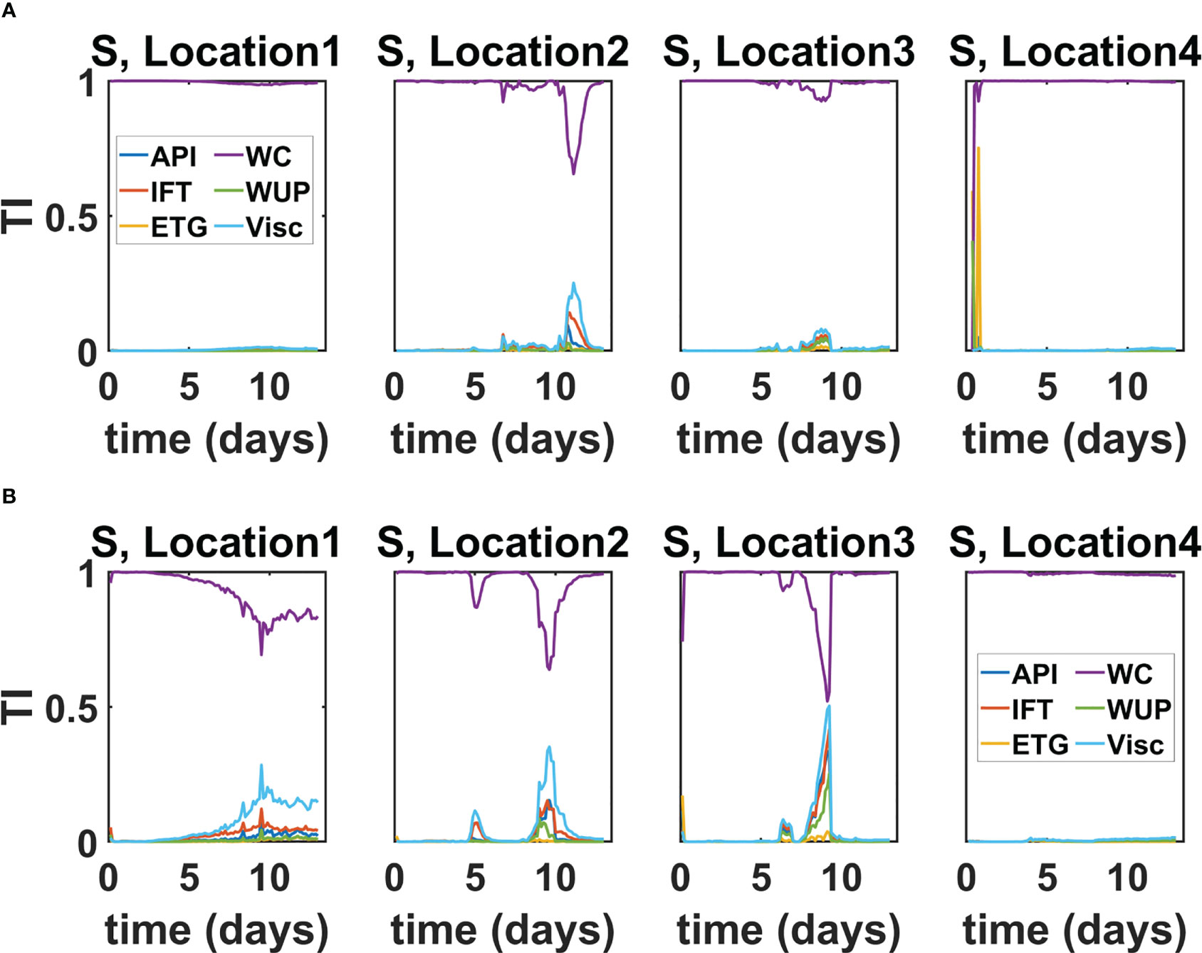
Figure 5 Evolution of the TI of (A) C Lon and (B) C Lat. Evolution curves are presented for the summer release scenarios from Locations 1–4.

These findings are consistent with and enhance well-established results in the literature, which have demonstrated that the transport of surface oil is strongly influenced by wind speed and direction and that wind stresses tend to elongate the surface of the oil slick in the direction of the surface winds (Androulidakis et al., 2018; Lodise et al., 2019; Duran et al., 2021). Our results provide quantitative estimates of the contribution of the uncertain variables on the location of the center of volume of the oil slick and allows to rule out uncertain parameters with lower contribution to the variability in the location of the center of volume. These results not only reveal that uncertainties in the wind coefficient dominate uncertainties in transport, but also indicate that all other uncertain parameters have a negligible contribution to the observed variabilities. Therefore, for the sake of predicting oil transport and estimating relevant confidence bounds, one could restrict the input space to the wind coefficient only, thus disregarding the remaining uncertain parameters.

The geometry of the oil slick is characterized using the central particle moments a, b, and c. We analyzed the variances of a, b, and c and generally observed that the prevailing behavior for C Lon and C Lat also holds for the second-order central particle moments. Figures 6A–C illustrate the evolution of the standard deviation of a, b, and c over the two-week release period. The curves outline a general increase in the variability of the central particle moments over time, except for the summer release scenario originating from release Location 3, which exhibits large oscillations. These oscillations may arise because the original release location is at the periphery of an eddy, inducing a rotational motion about its core.

FIGURE 6

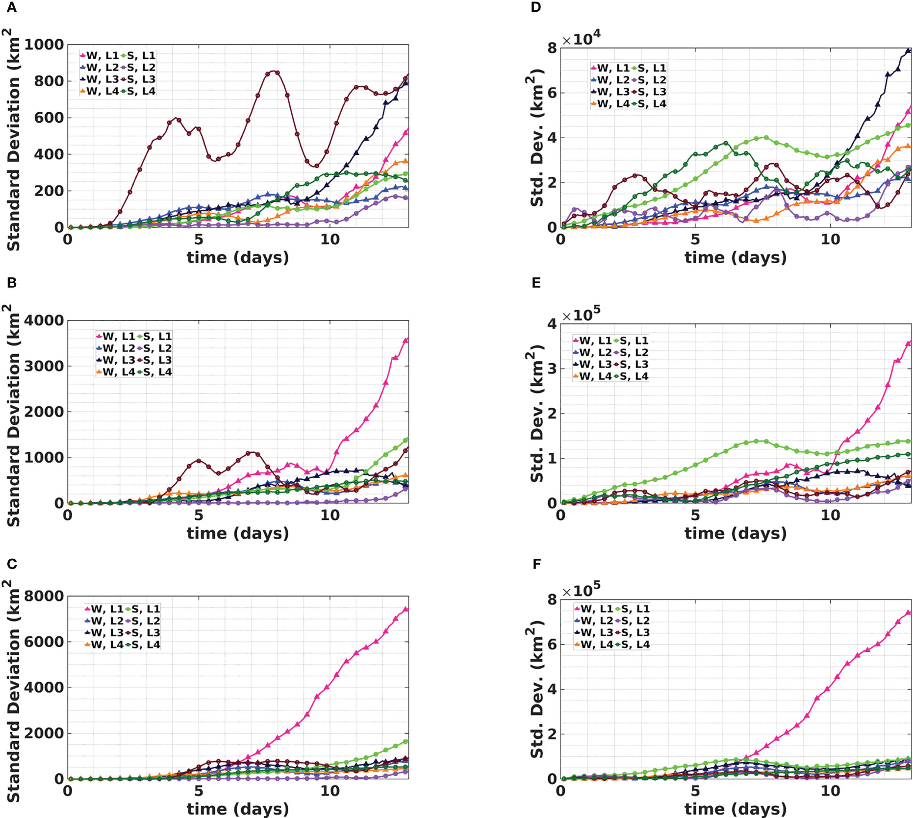
Figure 6 (A–C) Evolution curves of the standard deviation of the “a”, “b”, and “c” variables for all considered release scenarios. (D–F) Evolution of the standard deviation of $\widehat{a}$, $\widehat{b}$, and $\widehat{c}$ for the summer release scenarios.

The standard deviation of a is significantly smaller than that of c, which may be attributed to the elongated shape of the RS basin. For a given spill scenario (i.e., when the spill location and metocean conditions are specified), the variability of all three second moments is dominated by the uncertainty of the wind coefficient. This result can be readily appreciated from Figure 7, displaying the evolution of the total sensitivity indices of the central particle moments for the summer release scenarios. Locations 1 and 2 display a nonmonotonic change in the total sensitivity, with the wind coefficient having the largest influence. This outcome is unsurprising because the shear stresses imposed by the surface winds stretch the oil slick along the main wind direction, directly distorting its shape (Kampouris et al., 2021). However, the effects of the IFT and viscosity are generally not negligible, as observed from the results for Locations 1 and 2. Empirical findings have suggested that more-viscous oils spread less than less-viscous oils (Olugbenga et al., 2020), explaining the observed sensitivity of the slick deformation to the oil viscosity. Moreover, the IFT directly influences surface oil spreading, ultimately affecting the shape of the oil slick and how it stretches under the action of surface currents (Winoto et al., 2014; Speight, 2020). These results indicate that uncertainties about the shape of the oil slicks are primarily dependent on the wind coefficient and to a lesser degree on IFT and viscosity, and that the contribution of the remaining parameters is negligible.

FIGURE 7

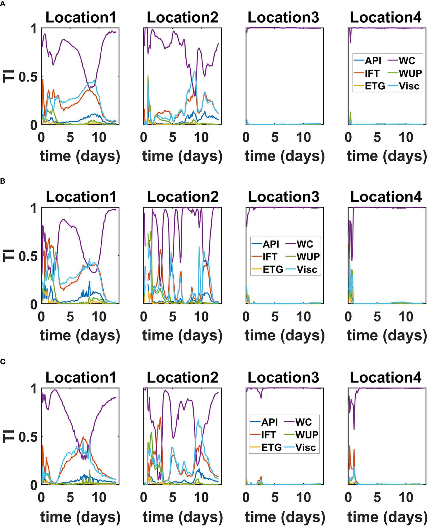
Figure 7 (A–C) Evolution curves of the total sensitivity indices corresponding to variables “a”, “b” and “c”, respectively, for the summer release scenarios.

As discussed in Section 2.3, we rely on the second-order nominal particle moments, $\widehat{a}$, $\widehat{b}$, and $\widehat{c}$ to characterize the properties of the elliptical region, centered at the centroid of the nominal oil slick, where spilled oil is likely to be present. Figures 6D–F illustrate the evolution of the standard deviation of $\widehat{a}$, $\widehat{b}$, and $\widehat{c}$ for all release scenarios. The evolution of the standard deviation of the nominal moments is similar to that of the central moments; however, the magnitude of the nominal particle moments is much larger than that of the central particle moments. This result is expected because the central particle moments measure the extent of the oil slick, whereas the nominal particle moments characterize the extent of the region centered on the centroid of the nominal oil slick, where individual oil slick realizations are likely to be present. The latter may be well separated from the nominal oil slick, explaining the higher values of the second-order nominal particle moments.

Unlike the variability of the central moments, which primarily depends on the wind coefficient and to lesser extent IFT and viscosity, the variability of the nominal moments is controlled by the wind coefficient. The total sensitivity indices (not shown)corresponding to the wind coefficient are approximately 1 for the entire simulation duration, and the remaining uncertainty parameters have total sensitivities close to zero. This behavior is unsurprising because the nominal moments reflect the combined effects of deformation (substantially affected by the wind coefficient) and mean motion (controlled by the wind coefficient). This approach substantially filters out the effects of IFT and viscosity, whose influence on the variability of the nominal moments can be deemed negligible. Thus, uncertainties in the second-order nominal particle moments are dominated solely by the wind coefficient.

4.3 Weathering quantities

This section analyzes the variability of the FME and FMD. The evolution of the standard deviation of the FME is reported in Figure 8A for all release scenarios. The figure indicates that the standard deviation of the FME increases monotonically as time progresses over a two-week period, with considerable variance after one week of the initial release. On the other hand, these predictions are fairly similar for the various release scenarios. As can be seen in Figure S3, the PDFs of FME also exhibit similar profiles, with widths increasing over time.

FIGURE 8

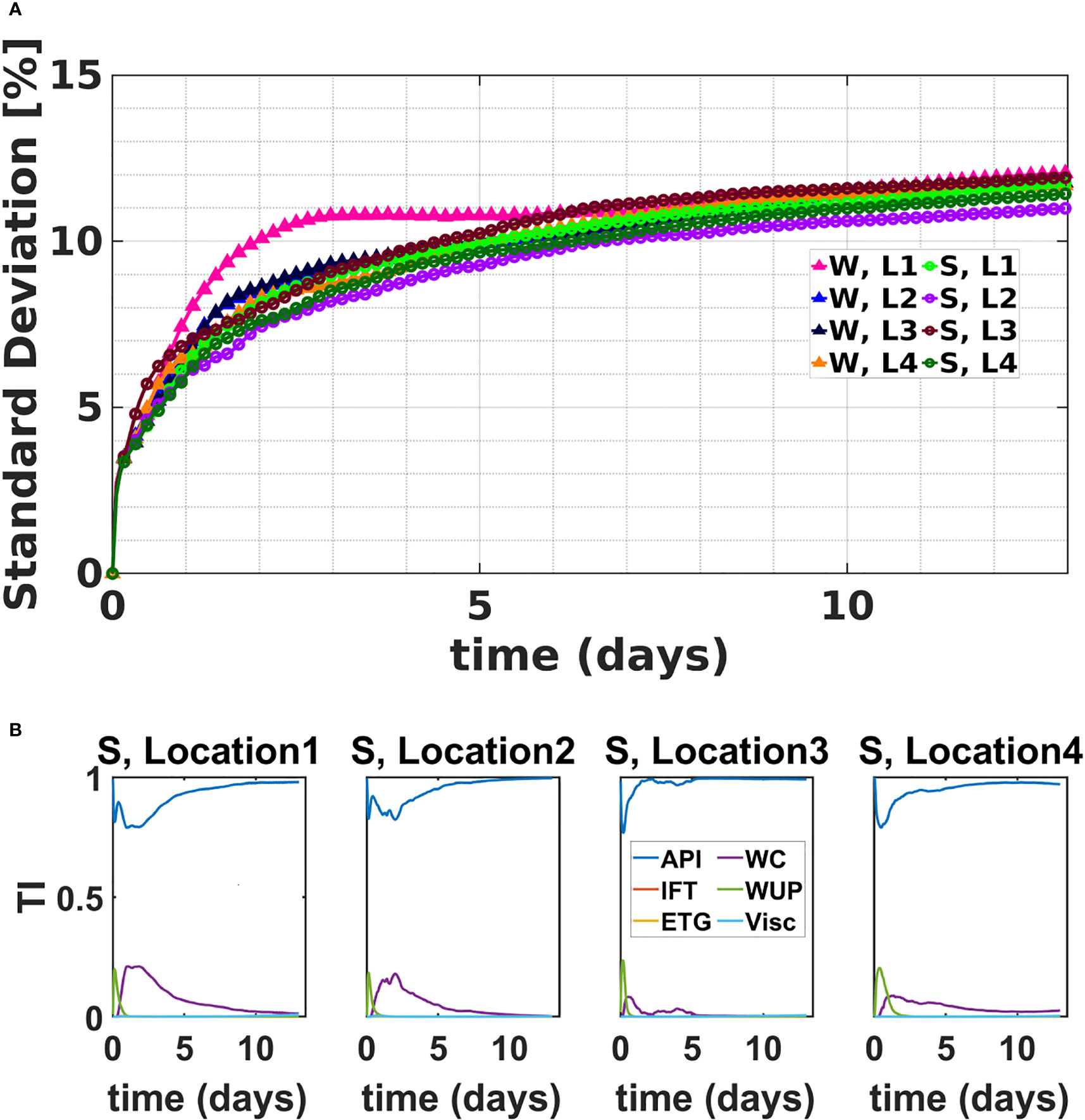
Figure 8 Evolution of the (A) standard deviation of the FME in time for all release scenarios considered. Subplot (B) illustrates the evolution of the total sensitivity indices of the FME corresponding to the summer release scenarios.

The evolution of the total sensitivity indices for the summer release scenarios is presented in Figure 8B. The curves demonstrate that, except for a short time following the release, the FME is most sensitive to the oil's API. The total sensitivity indices corresponding to the wind coefficient also appear to be more significant than the other uncertainty parameters; however, the influence of the wind coefficient on the FME is secondary compared to the API. These observations are consistent with the findings by (French-McCay et al., 2021), and also indicate that except at early times following the release, the variance of FME is dominated by uncertainty in API, and that contributions from other sources can be neglected.

Figure 9 presents a scatterplot of the 600 FME values predicted by MOHID one week after the initial release of oil from Location 1 for the winter and summer scenarios. The figure also illustrates the conditional expectation of FME and the 10^th and 90^th percentiles for varying obtained from the PC surrogate. The plots reveal that the FME increases nearly linearly with increasing. Realizations falling below the 10^th percentile curves exhibit a larger scatter compared with realizations falling above the 90^th percentile curves. This result is consistent with the skewness of the PDFs and the structure of their tails (see Figure S3). We examined the origin of these events by examining their parameters. The analysis indicated that extreme FME values correlate with extreme values of the wind coefficient. As expected, due to convective effects induced by surface winds, low FME values occur for low values of the wind coefficient and vice versa for higher wind coefficient values, which aligns with the results from (Saltymakova et al., 2020).

FIGURE 9

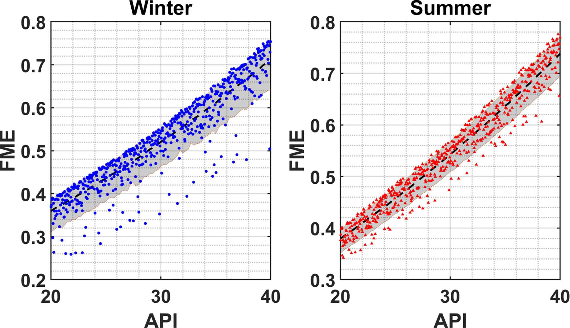
Figure 9 Scatterplot of the FME value one week after the initial release of oil from Location 1 for the summer and winter release scenarios, as predicted by MOHID. The figure also portrays the projection of the mean (black dashed line) and the 10^th (lower boundary of the shaded area) and 90 ^th (upper boundary of the shaded area) percentiles of the FME for values.

Figure 10A illustrates the evolution of the standard deviation of the FMD for all considered release scenarios. The figure indicates that the standard deviation of the FMD increases monotonically over time. The standard deviation estimated from the PC surrogate is comparable to the empirical standard deviation; however, the empirical standard deviation is smoother than that of the PC surrogate, possibly due to the cross-validation strategy adopted to obtain the PC coefficients. The results also reveal that the standard deviations vary substantially across various release scenarios, indicating that uncertainty in the input parameters over the considered ranges leads to appreciable relative differences in the FMD estimates. Overall, however, the FMD estimates exhibit small values in all scenarios considered, despite the large coefficients of variation. This is consistent with the empirical PDFs plotted in Figure S4. In contrast to the FME, the FMD PDFs reveal long-tailed unimodal distributions peaking at a small values (< 1%).

FIGURE 10

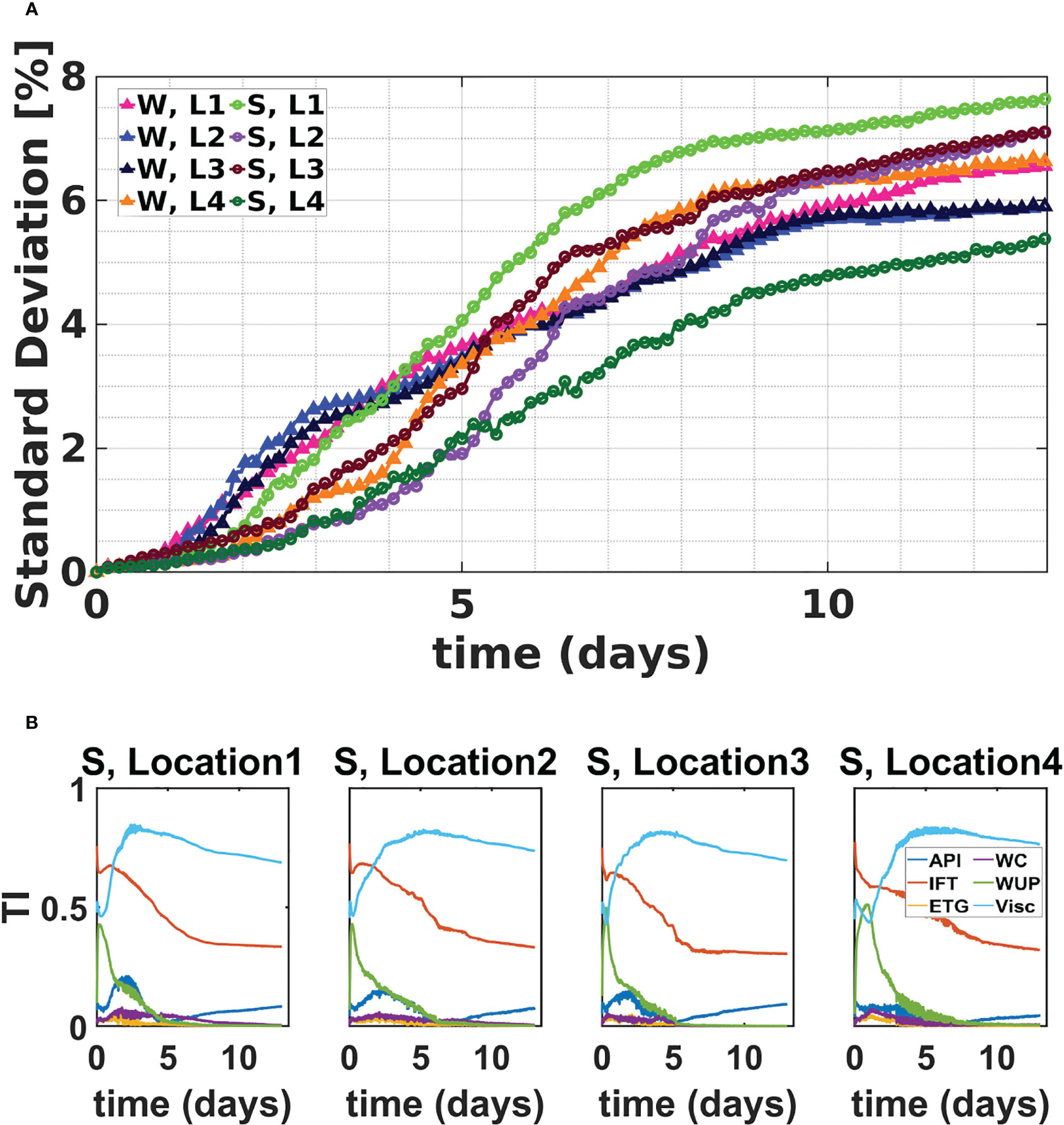
Figure 10 Evolution of the (A) standard deviation of the FMD in time. This plot presents the results for all considered release scenarios. Subplot (B) illustrates the evolution of the total sensitivity indices of the FME corresponding to the summer release scenarios.

The evolution of the total sensitivity indices of the FMD for all summer release scenarios is presented in Figure 10B. Initially, the IFT exhibits the highest total sensitivity index. As time progresses, the total sensitivity index of the IFT decreases to just below 0.5; thus, the IFT remains significant throughout the release. The FMD is also initially sensitive to the water uptake parameter after the oil release; however, it becomes insignificant later. The sensitivity of the FMD to viscosity increases with time, and the total sensitivity index of viscosity becomes the largest parameter and remains so over the remaining simulation time. Because the standard deviation of the FMD is very small in the first two days following the release, for the range of considered scenarios, the variability of the FMD is primarily sensitive to viscosity and IFT. The sensitivity of the FMD to the IFT may also be anticipated because the IFT affects the oil breakup dynamics and, consequently, the dispersion into the water column, as suggested from the observations by (Delvigne and Sweeney, 1988).

Note in the cases of FME and transport QoIs the analysis revealed the presence of a dominant parameter, but in the case of FMD multiple parameters have significant contributions to the variance. This leads us to examine the behavior of higher order sensitivities in this instance. Figure S5 illustrates the evolution the evolution of the first-order and second-order Sobol sensitivity indices for FMD. The results indicate that in addition to direct contributions from the uncertainty in IFT and viscosity, the mixed (cross-sensitivity) term between the IFT and viscosity also has significant impact. Thus, the contributions of these two dominant sources of uncertainty are clearly not additive.

A summary of the GSA results for the summer scenarios is presented in Table 4. The table present the average total sensitivity index for each QoI for each uncertainty parameter for the summer releases, respectively. As indicated, the total sensitivities are averaged over the release locations and across various time spans. Specifically, sensitivity values are averaged over early (≤ 3 days), intermediate (> 3 and< 10 days), and late (≥ 10 days) integration periods to further aid in identifying the uncertain input to which the QoI is most sensitive. Consistent with earlier discussions, for all considered time ranges, the location and geometry of the oil slick are most sensitive to the wind coefficient, and the variability of the FME is predominantly affected by the API. In contrast, the FMD exhibits strong sensitivity to viscosity and IFT. The results corresponding to the winter release exhibited similar behaviors and are presented in Table S2.

TABLE 4

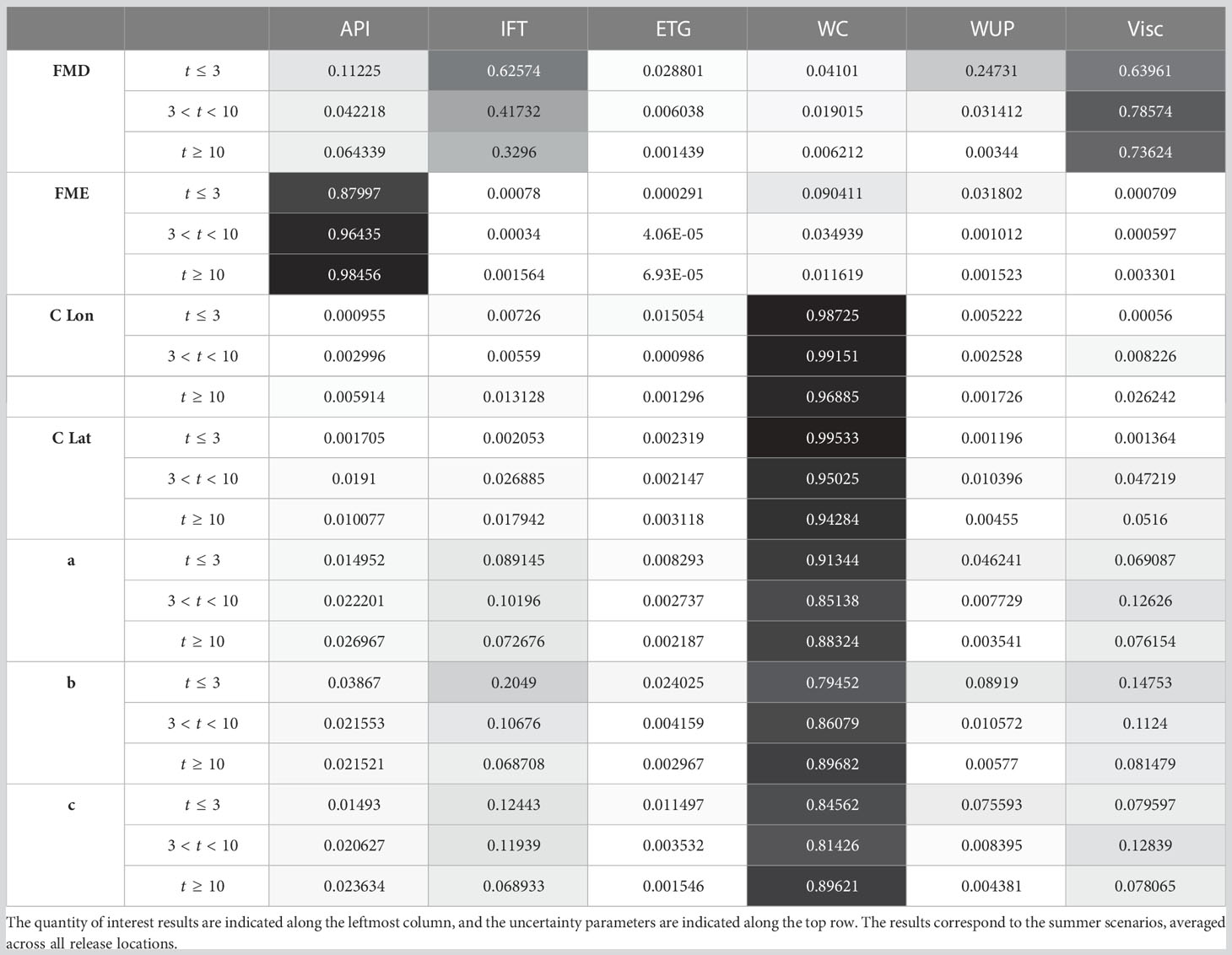
Table 4 Table listing the average total sensitivity indices for short (≤ 3 days), intermediate (> 3 days and< 10 days), and long (≥ 10 days) term.

5 Conclusion

We considered eight scenarios for oil spill incidents in the RS by specifying four release locations and two metocean conditions characteristic of winter and summer. For each scenario, the evolution of the released oil is simulated using the MOHID oil spill model over two weeks following the release.

Six uncertainty parameters that strongly influence the evolution of the oil were selected following a preliminary screening study. The six uncertain inputs include oil properties and oil-model parameters, including the API gravity (API), interfacial tension (IFT), empirical thickness gradient (ETG), wind coefficient (WC), water uptake parameter (WUP), and viscosity. We constructed PC surrogates of QoIs characterizing the location and geometry of the slick as well as weathering effects. A nonintrusive, regularized regression approach was used for this purpose. We analyzed the suitability of the surrogate models by quantifying the representation errors and exploited them to investigate the variability, distribution, and sensitivity of the QoIs.

In particular, the study indicated that, for the range of considered scenarios, QoIs characterizing the motion and deformation of the oil slick generally have large variances and exhibit strong dependence on metocean conditions. For a given scenario, the analysis demonstrated that the wind coefficient generally controls the influence of the motion and deformation of the oil slick. Specifically, the wind coefficient governs the variability in the centroid and nominal particle moments of the oil slick. The effects of viscosity and IFT are not negligible to determine the variability of the central particle moments. The analysis also indicated that the variability of FME is controlled by the API, with higher FME values for summer scenarios than for winter scenarios, as expected. Extreme values of the FME are positively correlated with extreme values of the wind coefficient. Finally, the results indicate that the variability of the FMD primarily depends on the oil viscosity followed by the IFT.

Overall, the present experiments indicate that, for the considered conditions, the prediction of areas affected by an accidental oil spill depends on metocean conditions and is highly sensitive to uncertainties in the metocean field and wind-coupling parametrization. For the range of tested conditions, the amount of oil affecting a region may be substantially affected by oil evaporation, which is highly sensitive to the API. For the assessment of spill effects over relatively short periods following an accidental release, these findings suggest that effective approaches can be conceived that focus primarily on metocean conditions, wind effects, evaporation, and their associated variabilities.

In conclusion, the present analysis focused on the influence of uncertainties in key oil properties and model parametrizations and ignored other sources of uncertainty, such as those affecting metocean conditions. In future work, we plan to account for these uncertainties using a flow ensemble approach while leveraging the results of the present study to restrict the number of uncertain oil and model parameters to a reasonably sized set. This plan would enable efficient means to simultaneously address forecasting and parameter uncertainties and effectively capitalize on the resulting predictions for impact assessments, source identification, or decision support.

Data availability statement

The raw data supporting the conclusions of this article will be made available by the authors, without undue reservation.

Author contributions

Conceptualization, MH, HM, and OK; Methodology, MH, HM, and OK; software, MH; validation, OL, IH, and OK; formal analysis, MH, HM, and OK; investigation, MH, HM, and OK; resources, IH and OK; data curation, MH and HM; writing—original draft preparation, MH, HM, and OK; writing—review and editing, MH, HM, OL, IH, and OK; visualization, MH and HM; supervision, OL, IH, and OK; project administration, OL, IH, and OK; funding acquisition, IH and OK. All authors contributed to the article and approved the submitted version.

Funding

This publication is based on work supported by the King Abdullah University of Science and Technology (KAUST) Office of Sponsored Research (OSR) under Award No. OSR-CRG2018-3711 and the Virtual Red Sea Initiative Award No. REP/1/3268-01-01.

Conflict of interest

The authors declare that the research was conducted in the absence of any commercial or financial relationships that could be construed as a potential conflict of interest.

Publisher’s note

All claims expressed in this article are solely those of the authors and do not necessarily represent those of their affiliated organizations, or those of the publisher, the editors and the reviewers. Any product that may be evaluated in this article, or claim that may be made by its manufacturer, is not guaranteed or endorsed by the publisher.

Supplementary material

The Supplementary Material for this article can be found online at: https://www.frontiersin.org/articles/10.3389/fmars.2023.1185106/full#supplementary-material

References

Abdul-Majeed G. H., Abu Al-Soof N. B. (2000). Estimation of gas–oil surface tension. J. Petroleum Sci. Eng. 27, 197–200. doi: 10.1016/S0920-4105(00)00058-9

CrossRef Full Text | Google Scholar

Abdul-Majeed G. H., Kattan R. R., Salman N. H. (1990). New correlation for estimating the viscosity of undersaturated crude oils. J. Can. Petroleum Technol. 29, 80–85. doi: 10.2118/90-03-10

CrossRef Full Text | Google Scholar

Adetula B., Bokov P. (2011). “Method for calculation of global sensitivity indices for few-group cross-section-dependent problems,” in International Conference on Mathematics and Computational Methods Applied to Nuclear Science and Engineering (M&C 2011), Rio de Janeiro, RJ, Brazil, American Nuclear Society (ANS).

Google Scholar

Alexanderian A., Winokur J., Sraj I., Srinivasan A., Iskandarani M., Thacker W. C., et al. (2012). Global sensitivity analysis in an ocean general circulation model: a sparse spectral projection approach. Comput. Geosciences 16, 757–778. doi: 10.1007/s10596-012-9286-2

CrossRef Full Text | Google Scholar

Alkhshall H., Westcott B. (2019). Iranian Oil tanker hit by two missiles near Saudi port: state news (Jeddah, Saudi Arabia: CNN).

Google Scholar

Al-Maamari R. S., Houache O., Abdul-Wahab S. A. (2006). New correlating parameter for the viscosity of heavy crude oils. Energy Fuels 20, 2586–2592. doi: 10.1021/ef0603030

CrossRef Full Text | Google Scholar

Alomair O., Jumaa M., Alkoriem A., Hamed M. (2015). Heavy oil viscosity and density prediction at normal and elevated temperatures. J. Petroleum Explor. Production Technol. 6, 253–263. doi: 10.1007/s13202-015-0184-8

CrossRef Full Text | Google Scholar

Androulidakis Y., Kourafalou V., Özgökmen T., Garcia-Pineda O., Lund B., Le Hénaff M., et al. (2018). Influence of river-induced fronts on hydrocarbon transport: a multiplatform observational study. J. Geophysical Research: Oceans 123, 3259–3285. doi: 10.1029/2017JC013514

CrossRef Full Text | Google Scholar

Barker C. H., Kourafalou V. H., Beegle-Krause C., Boufadel M., Bourassa M. A., Buschang S. G., et al. (2020). Progress in operational modeling in support of oil spill response. J. Mar. Sci. Eng. 8. doi: 10.3390/jmse8090668

CrossRef Full Text | Google Scholar

Carvalho S., Kürten B., Krokos G., Hoteit I., Ellis J. (2019). “Chapter 3 - the red sea,” in World seas: an environmental evaluation, 2nd ed. Ed Sheppard C. (Academic Press), 49–74.

Google Scholar

Chiffings A. W., Bleakley C., Kelleher G., Wells S. (1995). Marine region 11 Arabian seas. (World bank group) 3, 39–71.

Google Scholar

Crestaux T., Le Maître O., Martinez J.-M. (2009). Polynomial chaos expansion for sensitivity analysis. Reliability Eng. System Saf. 94, 1161–1172. doi: 10.1016/j.ress.2008.10.008

CrossRef Full Text | Google Scholar

Dasari H. P., Desamsetti S., Langodan S., Attada R., Kunchala R. K., Viswanadhapalli Y., et al. (2019). High-resolution assessment of solar energy resources over the arabian peninsula. Appl. Energy 248, 354–371. doi: 10.1016/j.apenergy.2019.04.105

CrossRef Full Text | Google Scholar

Debusschere B., Sargsyan K., Safta C., Chowdhary K. (2017). Uncertainty quantification toolkit (UQTk) (Cham: Springer International Publishing), 1807–1827. doi: 10.1007/978-3-319-12385-1_56

CrossRef Full Text | Google Scholar

De Dominicis M., Pinardi N., Zodiatis G., Archetti R. (2013a). Medslik-ii, a lagrangian marine surface oil spill model for short-term forecasting – part 2: numerical simulations and validations. Geoscientific Model. Dev. 6, 1871–1888. doi: 10.5194/gmd-6-1871-2013

CrossRef Full Text | Google Scholar

De Dominicis M., Pinardi N., Zodiatis G., Lardner R. (2013b). Medslik-ii, a lagrangian marine surface oil spill model for short-term forecasting – part 1: theory. Geoscientific Model. Dev. 6, 1851–1869. doi: 10.5194/gmd-6-1851-2013

CrossRef Full Text | Google Scholar

Dee D. P., Uppala S. M., Simmons A. J., Berrisford P., Poli P., Kobayashi S., et al. (2011). The era-interim reanalysis: configuration and performance of the data assimilation system. Q. J. R. Meteorological Soc. 137, 553–597. doi: 10.1002/qj.828

CrossRef Full Text | Google Scholar

Deguillard E., Pannacci N., Creton B., Rousseau B. (2013). Interfacial tension in oil–water–surfactant systems: on the role of intra-molecular forces on interfacial tension values using DPD simulations. J. Chem. Phys. 138, 144102. doi: 10.1063/1.4799888

PubMed Abstract | CrossRef Full Text | Google Scholar

Delvigne G., Sweeney C. (1988). Natural dispersion of oil. Oil Chem. pollut. 4, 281–310. doi: 10.1016/S0269-8579(88)80003-0

CrossRef Full Text | Google Scholar

Dong Y., Liu Y., Hu C., MacDonald I. R., Lu Y. (2022). Chronic oiling in global oceans. Science 376, 1300–1304. doi: 10.1126/science.abm5940

PubMed Abstract | CrossRef Full Text | Google Scholar

Duran R., Nordam T., Serra M., Barker C. (2021). “Chapter 3 - horizontal transport in oil-spill modeling,” in Marine hydrocarbon spill assessments. Ed. Makarynskyy O. (Amsterdam, Netherlands: Elsevier), 59–96.

Google Scholar

Eldred M. (2009). “Recent advances in non-intrusive polynomial chaos and stochastic collocation methods for uncertainty analysis and design,” in 50th AIAA/ASME/ASCE/AHS/ASC structures, structural dynamics, and materials conference (Palm Springs, California, United States of America: AIAA). doi: 10.2514/6.2009-2274

CrossRef Full Text | Google Scholar

Fay J. A. (1969). The spread of oil slicks on a calm Sea (Boston, MA: Springer US), 53–63.

Google Scholar

Fernandez M. (2010). Wind coefficients and model calibration for drifter trajectories simulation with MOHID. tech. rep. WP2 (Lisbon, Portugal: AMPERA). Europe windCoefficient.

Google Scholar

Fingas M. (1995). Water-in-oil emulsion formation: a review of physics and mathematical modelling. Spill Sci. Technol. Bull. 2, 55–59. doi: 10.1016/1353-2561(95)94483-Z

CrossRef Full Text | Google Scholar

Fingas M., Fieldhouse B. (2014). Water-in-Oil emulsions Vol. 8 (Hoboken, New Jersey: John Wiley & Sons, Ltd), 225–270. doi: 10.1002/9781118989982.ch8

CrossRef Full Text | Google Scholar

Fogang L. T., Kamal M. S., Hussain S. M. S., Kalam S., Patil S. (2020). Oil/water interfacial tension in the presence of novel polyoxyethylene cationic gemini surfactants: impact of spacer length, unsaturation, and aromaticity. Energy Fuels 34, 5545–5552. doi: 10.1021/acs.energyfuels.0c00044

CrossRef Full Text | Google Scholar

French-McCay D. P., Jayko K., Li Z., Spaulding M. L., Crowley D., Mendelsohn D., et al. (2021). Oil fate and mass balance for the deepwater horizon oil spill. Mar. pollut. Bull. 171, 112681. doi: 10.1016/j.marpolbul.2021.112681

PubMed Abstract | CrossRef Full Text | Google Scholar

Geary E. (2017). The API gravity of crude oil produced in the U.S. varies widely across states - today in energy - U.S (USA: Energy Information Administration (EIA)).

Google Scholar

Ghanem R. G., Spanos P. D. (1991). Stochastic finite elements: a spectral approach (New York, NY, USA: Springer New York).

Google Scholar

Goncalves R. C., Iskandarani M., Srinivasan A., Thacker W. C., Chassignet E., Knio O. M. (2016). A framework to quantify uncertainty in simulations of oil transport in the ocean. J. Geophysical Research: Oceans 121, 2058–2077. doi: 10.1002/2015JC011311

CrossRef Full Text | Google Scholar

Hadigol M., Doostan A. (2018). Least squares polynomial chaos expansion: a review of sampling strategies. Comput. Methods Appl. Mechanics Eng. 332, 382–407. doi: 10.1016/j.cma.2017.12.019

CrossRef Full Text | Google Scholar

Hodges B. R., Orfila A., Sayol J. M., Hou X. (2015). “Operational oil spill modelling: from science to engineering applications in the presence of uncertainty,” in Mathematical modelling and numerical simulation of oil pollution problems. Ed. Ehrhardt M. (Cham: Springer International Publishing), 99–126.

Google Scholar

Hollebone B. P. (2014). Appendix a the oil properties data appendix (Hoboken, New Jersey: John Wiley & Sons, Ltd), 575–681. doi: 10.1002/9781118989982.app1

CrossRef Full Text | Google Scholar

Homma T., Saltelli A. (1996). Importance measures in global sensitivity analysis of nonlinear models. Reliability Eng. System Saf. 52, 1–17. doi: 10.1016/0951-8320(96)00002-6

CrossRef Full Text | Google Scholar

Hoteit I., Abualnaja Y., Afzal S., Ait-El-Fquih B., Akylas T., Antony C., et al. (2021). Towards an end-to-end analysis and prediction system for weather, climate, and marine applications in the red sea. Bull. Am. Meteorological Soc. 102, E99–E122. doi: 10.1175/BAMS-D-19-0005.1

CrossRef Full Text | Google Scholar

Huan X., Safta C., Sargsyan K., Geraci G., Eldred M. S., Vane Z. P., et al. (2018). Global sensitivity analysis and estimation of model error, toward uncertainty quantification in scramjet computations. AIAA J. 56, 1170–1184. doi: 10.2514/1.J056278

CrossRef Full Text | Google Scholar

Iskandarani M., Le Hénaff M., Thacker W. C., Srinivasan A., Knio O. M. (2016a). Quantifying uncertainty in gulf of mexico forecasts stemming from uncertain initial conditions. J. Geophysical Research: Oceans 121, 4819–4832. doi: 10.1002/2015JC011573

CrossRef Full Text | Google Scholar

Iskandarani M., Wang S., Srinivasan A., Carlisle Thacker W., Winokur J., Knio O. M. (2016b). An overview of uncertainty quantification techniques with application to oceanic and oil-spill simulations. J. Geophysical Research: Oceans 121, 2789–2808. doi: 10.1002/2015JC011366

CrossRef Full Text | Google Scholar

Janeiro J., Martins F., Relvas P. (2012). Towards the development of an operational tool for oil spills management in the algarve coast. J. Coast. Conserv. 16, 449–460. doi: 10.1007/s11852-012-0201-8

CrossRef Full Text | Google Scholar

Kako S., Isobe A., Magome S., Hinata H., Seino S., Kojima A. (2011). Establishment of numerical beach-litter hindcast/forecast models: an application to goto islands, japan. Mar. pollut. Bull. 62, 293–302. doi: 10.1016/j.marpolbul.2010.10.011

PubMed Abstract | CrossRef Full Text | Google Scholar

Kampouris K., Vervatis V., Karagiorgos J., Sofianos S. (2021). Oil spill model uncertainty quantification using an atmospheric ensemble. Ocean Sci. 17, 919–934. doi: 10.5194/os-17-919-2021

CrossRef Full Text | Google Scholar

KC U., Aryal J., Garg S., Hilton J. (2021). Global sensitivity analysis for uncertainty quantification in fire spread models. Environ. Model. Software 143, 105110. doi: 10.1016/j.envsoft.2021.105110

CrossRef Full Text | Google Scholar

Keramea P., Spanoudaki K., Zodiatis G., Gikas G., Sylaios G. (2021). Oil spill modeling: a critical review on current trends, perspectives, and challenges. J. Mar. Sci. Eng. 9. doi: 10.3390/jmse9020181

CrossRef Full Text | Google Scholar

Khan S., Al-Marhoun M., Duffuaa S., Abu-Khamsin S. (1987). “Viscosity correlations for saudi arabian crude oils,” in All days (Bahrain: SPE), 1–8.

Google Scholar

Kleinhaus K., Voolstra C. R., Meibom A., Amitai Y., Gildor H., Fine M. (2020). A closing window of opportunity to save a unique marine ecosystem. Front. Mar. Sci. 7, 1117. doi: 10.3389/fmars.2020.615733

CrossRef Full Text | Google Scholar

Knio O., Le Maître O. (2006). Uncertainty propagation in cfd using polynomial chaos decomposition. Fluid Dynamics Res. 38, 616–640. Recent Topics in Computational Fluid Dynamics. doi: 10.1016/j.fluiddyn.2005.12.003

CrossRef Full Text | Google Scholar

Kostianaia E. A., Kostianoy A., Lavrova O. Y., Soloviev D. M. (2020). Oil pollution in the northern red Sea: a threat to the marine environment and tourism development (Cham: Springer International Publishing), 329–362.

Google Scholar

Langodan S., Cavaleri L., Vishwanadhapalli Y., Pomaro A., Bertotti L., Hoteit I. (2017). The climatology of the red sea – part 1: the wind. Int. J. Climatology 37, 4509–4517. doi: 10.1002/joc.5103

CrossRef Full Text | Google Scholar

Langodan S., Cavaleri L., Viswanadhapalli Y., Hoteit I. (2014). The red sea: a natural laboratory for wind and wave modeling. J. Phys. Oceanography 44, 3139–3159. doi: 10.1175/JPO-D-13-0242.1

CrossRef Full Text | Google Scholar

Laurie D. (1997). Calculation of gauss-kronrod quadrature rules. Math. Comput. 66, 1133–1145. doi: 10.1090/S0025-5718-97-00861-2

CrossRef Full Text | Google Scholar

Lehr W., Jones R., Evans M., Simecek-Beatty D., Overstreet R. (2002). Revisions of the ADIOS oil spill model. Environ. Model. Software 17, 189–197. doi: 10.1016/S1364-8152(01)00064-0

CrossRef Full Text | Google Scholar

Leitao P., Malhadas M., Ribeiro J., Leitao J., Pierini J., Otero L. (2013). An overview for simulating the blowout of oil spills with a three-dimensional model approach (Caribbean Coast, Colombia: IST press), 97–115.

Google Scholar

Le Maître O., Knio O. (2010). Spectral methods for uncertainty quantification (Netherlands: Springer Netherlands).

Google Scholar

Li S. (2017). Evaluation of new weathering algorithms for oil spill modeling (Halifax, Canada: Dalhousie University). Master’s thesis.

Google Scholar

Ling K., He J. (2012). “A new correlation to calculate oil-water interfacial tension,” in All days (Kuwait City, Kuwait: SPE), 1–9.

Google Scholar

Lodise J., Özgökmen T., Griffa A., Berta M. (2019). ). vertical structure of ocean surface currents under high winds from massive arrays of drifters. Ocean Sci. 15, 1627–1651. doi: 10.5194/os-15-1627-2019

CrossRef Full Text | Google Scholar

Lopes I. E. (2016). Uncertainty analysis in oil spill modelling – sensitivity and forcing analysis for a spill in the Portuguese coast and tagus estuary (Lisbon, Portugal: Técnico Lisboa). Master’s thesis.

Google Scholar

Lord D., Allen R., Rudeen D., Wocken C., Aulich T. (2018). DOE/DOT crude oil characterization research study, task 2 test report on evaluating crude oil sampling and analysis methods, revision 1 - winter sampling. doi: 10.2172/1458999

CrossRef Full Text | Google Scholar

Lüdtke N., Panzeri S., Brown M., Broomhead D. S., Knowles J., Montemurro M. A., et al. (2008). ). information-theoretic sensitivity analysis: a general method for credit assignment in complex networks. J. R. Soc. Interface 5, 223–235. doi: 10.1098/rsif.2007.1079

PubMed Abstract | CrossRef Full Text | Google Scholar

Lüthen N., Marelli S., Sudret B. (2021). Sparse polynomial chaos expansions: literature survey and benchmark. SIAM/ASA J. Uncertainty Quantification 9, 593–649. doi: 10.1137/20M1315774

CrossRef Full Text | Google Scholar

Mackay D., Zagorski W. (1981). “EnglishStudies of the formation of water-in-Oil emulsions,” in Fourth Arctic marine oilspill program technical seminar, vol. 75. (Environment Canada, Ottawa: Edmonton, Alberta).

Google Scholar

Mackay D., Zagorski W. (1982). “EnglishWater-in-Oil emulsions: a stability hypothesis,” in 5th Arctic marine oilspill program technical seminar (Environment Canada, Ottawa: Edmonton, Alberta), 61–74.

Google Scholar

Marelli S., Sudret B. (2014). “Uqlab: a framework for uncertainty quantification in matlab,” in Vulnerability, uncertainty, and risk (University of Liverpool, United Kingdom: ASCE), 2554–2563. doi: 10.1061/9780784413609.257

CrossRef Full Text | Google Scholar

Marshall J., Hill C., Perelman L., Adcroft A. (1997). Hydrostatic, quasi-hydrostatic, and nonhydrostatic ocean modeling. . J. Geophysical Research: Oceans 102, 5733–5752. doi: 10.1029/96JC02776

CrossRef Full Text | Google Scholar

Martorell S., Soares C. G., Barnett J. (2008). Safety, reliability and risk analysis (London: CRC Press). doi: 10.1201/9781482266481

CrossRef Full Text | Google Scholar

Mateus M. D., Franz G. (2015). Sensitivity analysis in a complex marine ecological model. Water 7, 2060–2081. doi: 10.3390/w7052060

CrossRef Full Text | Google Scholar

Maximenko N., Hafner J., Niiler P. (2012). Pathways of marine debris derived from trajectories of lagrangian drifters. Mar. Pollut. Bull. 65, 51–62. doi: 10.1016/j.marpolbul.2011.04.016

PubMed Abstract | CrossRef Full Text | Google Scholar

Mishra A. K., Kumar G. S. (2015). Weathering of oil spill: modeling and analysis. Aquat. Proc. 4, 435–442. doi: 10.1016/j.aqpro.2015.02.058

CrossRef Full Text | Google Scholar

Mittal H. V. R., Langodan S., Zhan P., Li S., Knio O., Hoteit I. (2021). Hazard assessment of oil spills along the main shipping lane in the red sea. Sci. Rep. 11, 17078. doi: 10.1038/s41598-021-96572-5

PubMed Abstract | CrossRef Full Text | Google Scholar

Najm H. N. (2009). Uncertainty quantification and polynomial chaos techniques in computational fluid dynamics. Annu. Rev. Fluid Mechanics 41, 35–52. doi: 10.1146/annurev.fluid.010908.165248

CrossRef Full Text | Google Scholar

Navarro Jimenez M., Le Maître O. P., Knio O. M. (2016). Global sensitivity analysis in stochastic simulators of uncertain reaction networks. J. Chem. Phys. 145, 244106. doi: 10.1063/1.4971797

PubMed Abstract | CrossRef Full Text | Google Scholar

Neves R. (1985). Biodimensional model for residual circulation in coastal zones: application to the sado estuary. Annales geophysicae (1983) 3, 465–471.

Google Scholar

Neves R. (2013). The mohid concept, ocean modelling for coastal management–case studies with mohid. MOHID's handbook 1–11.

Google Scholar

Obuchi T., Kabashima Y. (2016). Cross validation in LASSO and its acceleration. J. Stat. Mechanics: Theory Experiment 2016, 053304. doi: 10.1088/1742-5468/2016/05/053304

CrossRef Full Text | Google Scholar

Oliveira A. R., Ramos T. B., Simionesei L., Pinto L., Neves R. (2020). Sensitivity analysis of the mohid-land hydrological model: a case study of the ulla river basin. Water 12. doi: 10.3390/w12113258

CrossRef Full Text | Google Scholar

Olugbenga A. G., Yahya M. D., Garba M. U., Mohammed A. (2020). Utilization of oil properties to develop a spreading rate regression model for nigerian crude oil. Adv. Chem. Eng. Sci. 10, 332–342. doi: 10.4236/aces.2020.104021

CrossRef Full Text | Google Scholar

Oudot J., Merlin F., Pinvidic P. (1998). Weathering rates of oil components in a bioremediation experiment in estuarine sediments. Mar. Environ. Res. 45, 113–125. doi: 10.1016/S0141-1136(97)00024-X

CrossRef Full Text | Google Scholar

Ranstam J., Cook J. A. (2018). LASSO regression. Br. J. Surg. 105, 1348–1348. doi: 10.1002/bjs.10895

CrossRef Full Text | Google Scholar

Reed M., Aamo O. M., Daling P. S. (1995). Quantitative analysis of alternate oil spill response strategies using oscar. Spill Sci. Technol. Bull. 2, 67–74. doi: 10.1016/1353-2561(95)00020-5

CrossRef Full Text | Google Scholar

Reed M., Johansen Øistein, Brandvik P. J., Daling P., Lewis A., Fiocco R., et al. (1999). Oil spill modeling towards the close of the 20th century: overview of the state of the art. Spill Sci. Technol. Bull. 5, 3–16. doi: 10.1016/S1353-2561(98)00029-2

CrossRef Full Text | Google Scholar

Reed M., Turner C., Odulo A. (1994). The role of wind and emulsification in modelling oil spill and surface drifter trajectories. Spill Sci. Technol. Bull. 1, 143–157. doi: 10.1016/1353-2561(94)90022-1

CrossRef Full Text | Google Scholar

Rocha L., Velho L., Carvalho P. (2002). “Image moments-based structuring and tracking of objects,” in Proceedings. XV Brazilian Symposium on Computer Graphics and Image Processing , Fortaleza, Brazil. 99–105. doi: 10.1109/SIBGRA.2002.1167130

CrossRef Full Text | Google Scholar

Roth V. (2004). The generalized lasso. IEEE Trans. Neural Networks 15, 16–28. doi: 10.1109/TNN.2003.809398

CrossRef Full Text | Google Scholar

Saltymakova D., Desmond D. S., Isleifson D., Firoozy N., Neusitzer T. D., Xu Z., et al. (2020). Effect of dissolution, evaporation, and photooxidation on crude oil chemical composition, dielectric properties and its radar signature in the arctic environment. Mar. pollut. Bull. 151, 110629. doi: 10.1016/j.marpolbul.2019.110629

PubMed Abstract | CrossRef Full Text | Google Scholar

Sánchez-Minero F., Sánchez-Reyna G., Ancheyta J., Marroquin G. (2014). Comparison of correlations based on api gravity for predicting viscosity of crude oils. Fuel 138, 193–199. doi: 10.1016/j.fuel.2014.08.022

CrossRef Full Text | Google Scholar

Schenk C. J., Pollastro R. M., Hill R. J. (2006). Natural bitumen resources of the united states. (Reston, VA, USA: USGS).

Google Scholar

Sobol I. M. (1993). EnglishSensitivity estimates for nonlinear mathematical models. Math. Model. Comput. Exper. 1, 407–414.

Google Scholar

Sobol I. (2001). Global sensitivity indices for nonlinear mathematical models and their monte carlo estimates. Mathematics Comput. Simulation 55, 271–280. doi: 10.1016/S0378-4754(00)00270-6

CrossRef Full Text | Google Scholar

Speight J. (2020). “Chapter 9 - analysis of oil from tight formations,” in Shale oil and gas production processes. Ed. Speight J. (Cambridge MA, United States: Gulf Professional Publishing), 519–571.

Google Scholar

Sraj I., Mandli K. T., Knio O. M., Dawson C. N., Hoteit I. (2017). Quantifying uncertainties in fault slip distribution during the tōhoku tsunami using polynomial chaos. Ocean Dynamics 67, 1535–1551. doi: 10.1007/s10236-017-1105-9

CrossRef Full Text | Google Scholar

Srinivasan A., LeHenaff M., Kourafalou V. H., Thacker W. C., Tsinoremas N. F., Helgers J., et al. (2010). “Many task computing for modeling the fate of oil discharged from the deep water horizon well blowout,” in 2010 3rd workshop on many-task computing on grids and supercomputers (New Orleans, LA, USA: IEEE), 1–7.

Google Scholar

Sudret B. (2008). Global sensitivity analysis using polynomial chaos expansions. Reliability Eng. System Saf. 93, 964–979. doi: 10.1016/j.ress.2007.04.002

CrossRef Full Text | Google Scholar

Thacker W. C., Iskandarani M., Gonçalves R. C., Srinivasan A., Knio O. M. (2015). Pragmatic aspects of uncertainty propagation: a conceptual review. Ocean Model. 95, 25–36. doi: 10.1016/j.ocemod.2015.09.001

CrossRef Full Text | Google Scholar

Tibshirani R. (1996). Regression shrinkage and selection via the lasso. J. R. Stat. Society. Ser. B (Methodological) 58, 267–288.

Google Scholar

Transportation Research Board and National Research Council (2003). Oil in the Sea III: inputs, fates, and effects Vol. 4 (Washington, DC: The National Academies Press), 89–117. doi: 10.17226/10388

CrossRef Full Text | Google Scholar

van Sebille E., Griffies S. M., Abernathey R., Adams T. P., Berloff P., Biastoch A., et al. (2018). Lagrangian Ocean analysis: fundamentals and practices. Ocean Model. 121, 49–75. doi: 10.1016/j.ocemod.2017.11.008

CrossRef Full Text | Google Scholar

Viswanadhapalli Y., Dasari H. P., Langodan S., Challa V. S., Hoteit I. (2017). Climatic features of the red sea from a regional assimilative model. Int. J. Climatology 37, 2563–2581. doi: 10.1002/joc.4865

CrossRef Full Text | Google Scholar

Wang S., Iskandarani M., Srinivasan A., Thacker W. C., Winokur J., Knio O. M. (2016). Propagation of uncertainty and sensitivity analysis in an integral oil-gas plume model. J. Geophysical Research: Oceans 121, 3488–3501. doi: 10.1002/2015JC011365

CrossRef Full Text | Google Scholar

Wang S.-D., Shen Y.-M., Guo Y.-K., Tang J. (2008). Three-dimensional numerical simulation for transport of oil spills in seas. Ocean Eng. 35, 503–510. doi: 10.1016/j.oceaneng.2007.12.001

CrossRef Full Text | Google Scholar

Whitson C. H., R Brule M. (2000). EnglishPhase behavior (Society of petroleum engineers of AIME: Henry l. doherty memorial fund of AIME, society of petroleum engineers). (Pennsylvania, USA: Society of Petroleum Engineers).

Google Scholar

Wiener N. (1938). The homogeneous chaos. Am. J. Mathematics 60, 897–936. doi: 10.2307/2371268

CrossRef Full Text | Google Scholar

Winokur J., Conrad P., Sraj I., Knio O., Srinivasan A., Thacker W. C., et al. (2013). A priori testing of sparse adaptive polynomial chaos expansions using an ocean general circulation model database. Comput. Geosciences 17, 899–911. doi: 10.1007/s10596-013-9361-3

CrossRef Full Text | Google Scholar

Winoto W., Loahardjo N., Takamura K., Morrow N. R. (2014). Spreading and retraction of spilled crude oil on seawater. Int. Oil Spill Conf. Proc. 2014, 1465–1473. doi: 10.7901/2169-3358-2014.1.1465

CrossRef Full Text | Google Scholar

Xu H.-L., Chen J.-N., Wang S.-D., Liu Y. (2012). ). oil spill forecast model based on uncertainty analysis: a case study of dalian oil spill. Ocean Eng. 54, 206–212. doi: 10.1016/j.oceaneng.2012.07.019

CrossRef Full Text | Google Scholar

Yao F., Hoteit I., Pratt L. J., Bower A. S., Köhl A., Gopalakrishnan G., et al. (2014a). Seasonal overturning circulation in the red sea: 2. winter circulation. J. Geophysical Research: Oceans 119, 2263–2289. doi: 10.1002/2013JC009004

CrossRef Full Text | Google Scholar

Yao F., Hoteit I., Pratt L. J., Bower A. S., Zhai P., Köhl A., et al. (2014b). Seasonal overturning circulation in the red sea: 1. model validation and summer circulation. J. Geophysical Research: Oceans 119, 2238–2262. doi: 10.1002/2013JC009331

CrossRef Full Text | Google Scholar

Zhan P., Krokos G., Guo D., Hoteit I. (2019). Three-dimensional signature of the red sea eddies and eddy-induced transport. Geophysical Res. Lett. 46, 2167–2177. doi: 10.1029/2018GL081387

CrossRef Full Text | Google Scholar

Zhan P., Subramanian A. C., Yao F., Kartadikaria A. R., Guo D., Hoteit I. (2016). The eddy kinetic energy budget in the red sea. J. Geophysical Research: Oceans 121, 4732–4747. doi: 10.1002/2015JC011589

CrossRef Full Text | Google Scholar

Zodiatis G., Lardner R., Spanoudaki K., Sofianos S., Radhakrishnan H., Coppini G., et al. (2021). “Chapter 5 - operational oil spill modelling assessments,” in Marine hydrocarbon spill assessments. Ed. Makarynskyy O. (Amsterdam, Netherlands: Elsevier), 145–197.

Google Scholar