Projecting shifts in the distributions of Chinese endemic vertebrate species under climate and land-use change

Deng, Yiming; Goodale, Eben; Dong, Anran; Jiang, Demeng; Jiang, Aiwu; Zhang, Zhixin; Mammides, Christos

doi:10.3389/fevo.2023.1174495

ORIGINAL RESEARCH article

Front. Ecol. Evol., 13 June 2023

Sec. Conservation and Restoration Ecology

Volume 11 - 2023 | https://doi.org/10.3389/fevo.2023.1174495

This article is part of the Research Topic Proceedings of INTECOL 2022: LOOK UP! CONSERVATION AND RESTORATION View all 6 articles

Projecting shifts in the distributions of Chinese endemic vertebrate species under climate and land-use change

Aiwu Jiang¹^*

Zhixin Zhang^4,5^*

Christos Mammides⁶

¹Guangxi Key Laboratory of Forest Ecology and Conservation, College of Forestry, Guangxi University, Nanning, Guangxi, China
²Department of Health and Environmental Sciences, Xi'an Jiaotong-Liverpool University, Suzhou, Jiangsu, China
³College of Urban and Environmental Science, Peking University, Beijing, China
⁴CAS Key Laboratory of Tropical Marine Bio-resources and Ecology, South China Sea Institute of Oceanology, Chinese Academy of Sciences, Guangzhou, Guangdong, China
⁵Global Ocean and Climate Research Center, South China Sea Institute of Oceanology, Guangzhou, Guangdong, China
⁶Nature Conservation Unit, Frederick University, Nicosia, Cyprus

Human-induced climate and land-use change impact species’ habitats and survival ability. A growing body of research uses species distribution models (SDMs) to predict potential changes in species ranges under global change. We constructed SDMs for 411 Chinese endemic vertebrates using Maximum Entropy (MaxEnt) modeling and four shared socioeconomic pathways (SSPs) spanning to 2100. We compared four different approaches: (1) using only climatic and geographic factors, (2) adding anthropogenic factors (land-use types and human population densities), but only using current data to project into the future, (3) incorporating future estimates of the anthropogenic variables, and (4) processing species occurrence data extracted from IUCN range maps to remove unsuitable areas and reflect each species’ area of habitat (AOH). The results showed that the performance of the models (as measured by the Boyce index) improved with the inclusion of anthropogenic data. Additionally, the predicted future suitable area was most restricted and diminished compared to the current area, when using the fourth approach. Overall, the results are consistent with other studies showing that species distributions will shift to higher elevations and latitudes under global change, especially under higher emission scenarios. Species threatened currently, as listed by the IUCN, will have their range decrease more than others. Additionally, higher emission scenarios forecast more threatened species in the future. Our findings show that approaches to optimizing SDM modeling can improve accuracy, predicting more direct global change consequences, which need to be anticipated. We also show that global change poses a significant threat to endemic species even in regions with extensive protected land at higher latitudes and elevations, such as China.

1. Introduction

Global biodiversity is threatened by a multitude of anthropogenic factors, including growing human populations, intensified land-use practices, and climate change (Devictor et al., 2008; Bellard et al., 2012; Williams et al., 2021). Improved biodiversity conservation measures are critical in the face of deteriorating ecological conditions (Araújo et al., 2019; Nielsen et al., 2021). In turn, to effectively design such measures, it is essential to accurately predict how species will shift their geographical distributions under global change (Bennett et al., 2017; Hanson et al., 2020; Hu et al., 2020).

Species distribution models (SDMs) are recognized as a powerful approach for predicting species’ geographical distribution patterns (Elith and Leathwick, 2009; Guisan et al., 2017; Zurell et al., 2020). SDMs are statistical modeling tools that quantify the relationships between species distributions and a collection of environmental and anthropogenic variables. Climate is frequently regarded as the primary driver of species distributions (Pearson and Dawson, 2003). Consequently, previous SDM studies aiming at predicting species distributions under global change have relied heavily on climatic variables (e.g., Devictor et al., 2008; Bellard et al., 2012).

A variety of other factors, however, also regulate species distributions, and it has been noted that climate-only models may yield imprecise predictions (Thuiller et al., 2004; Martin et al., 2013). Further, it has been recommended that anthropogenic factors, in particular, should also be incorporated into SDMs (Jetz et al., 2007; Nori et al., 2018). Moreover, even in cases in which such variables are included, the conceptual and technical challenges associated with predicting their future conditions, such as future land-use patterns, have forced many studies to base their modeling on static data that reflect only current patterns (Verburg et al., 2011). Yet, updated future estimates of anthropogenic factors are now increasingly becoming available, and hence their dynamic nature should be explored in SDMs (Stanton et al., 2012; Martin et al., 2013; Milanesi et al., 2020).

Another aspect of SDMs that has been recently discussed is related to species distribution data (Merow et al., 2013). There are mainly two types of distribution data in SDM studies: occurrence records obtained from public records and databases, such as the Global Biodiversity Information Facility (GBIF), and occurrences extracted from the species IUCN ranges (Fourcade, 2016). Species occurrences derived primarily from museum records and public databases have been shown to suffer from sampling biases (Hughes et al., 2021). Therefore, species range polygons have been often used as additional distribution data to avoid biased estimations of species realized niches, particularly in studies involving large numbers of species (Fourcade, 2016; Thuiller et al., 2019). However, it has been pointed out that range polygons, such as those available by the IUCN, tend to considerably overestimate the occurrence of species as commission errors (Ocampo-Peñuela et al., 2016; Brooks et al., 2019; Jung et al., 2020). These methods can overestimate the species’ available suitable habitat, also known as the Area of Habitat (AOH), by including elevations or habitats that the species are known not to inhabit (Supplementary Figure 2) (Brooks et al., 2019; Jung et al., 2020). Consequently, more studies are needed to explore whether range polygons that account for AOH can improve the accuracy of SDM predictions.

China is a megadiverse country, so adequately protecting its biodiversity is crucial (China Catalogue of Life, 2020). However, China is also the most populous country and has witnessed tremendous anthropogenic changes in recent centuries (He et al., 2013). Moreover, China is expected to face significant land-use changes in the near future due to increased urbanization (Zhao et al., 2006; Dong et al., 2019) and other social and environmental factors, including climatic change (Shukla et al., 2018; Spinoni et al., 2019). Earlier studies on predicting the effects of global change on Chinese endemic vertebrates have focused mainly on climatic variables without necessarily considering anthropogenic impacts (Li et al., 2013; Hu et al., 2020; Wu, 2020). That said, a recent article did consider anthropogenic influences in an SDM model, but focused only on a single plant species (Tang and Zhao, 2022).

In this study, we compared four different approaches for predicting the potential effects of global anthropogenic land use and climate change on Chinese endemic vertebrate species. The first approach included climatic and geographic variables only, such as temperature, precipitation, aspect, and slope. The second approach included also anthropogenic variables, specifically current human population densities and land-use patterns, but the data was static (i.e., used only current patterns). The third approach included future human population densities and future land-use patterns and thus is dynamic. These three approaches (1, 2, 3) were applied to occurrence data from multiple sources, including occurrences extracted from the IUCN species ranges, by randomly selecting points within the distribution of each species. We also investigated a fourth approach, similar to the third, but in which unsuitable habitats and elevations were removed in order to maintain each species’ AOH (Forero-Medina et al., 2011; Brooks et al., 2019). We hypothesized that: (a) the inclusion of anthropogenic variables and the approach of eliminating unsuitable habitats within the IUCN range (i.e., maintaining only the AOH) would improve model performance, (b) the inclusion of dynamic anthropogenic variables would predict smaller suitable areas in the current situation, and more profound range loss in the future, as many species are not able to tolerate human-modified and human-dominated land-types.

2. Methods

2.1. Species occurrence data

China is home to 641 endemic terrestrial vertebrate species, including 272 amphibians, 77 birds, 150 mammals, and 142 reptiles (China Animal Scientific Database, 2020¹; IUCN, 2022). Aquatic species have vastly different environmental preferences, constraints, and movement patterns, so they were excluded from this study (Sundblad et al., 2009; Zhang et al., 2020). To determine the distributions of the rest of the Chinese endemic vertebrate species (n = 411), we compiled a dataset of the geographic coordinates of the species occurrences obtained from the Global Biodiversity Information Facility (GBIF: www.gbif.org), the IUCN range maps (www.iucnredlist.org), and the Chinese Bird Report (www.birdreport.cn).

To predict species distributions using the first three approaches (approaches 1–3), we first extracted occurrence records from the IUCN range maps (Van Wilgen et al., 2009; Fourcade, 2016; Sales et al., 2017) by randomly selecting records within each species’ range, with the number of points being proportional to the species’ range size. This was necessary to avoid overfill and possibly exaggerate the species’ niches due to extensive point data (Sales et al., 2019). Specifically, for species that occupied less than 100 grid cells (each of 2.5 arc-minutes square, roughly equal to 5 km² at the equator), we selected all occurrence points within the IUCN polygon range; for species with 101 to 500 cells, we randomly selected 50% of the points; similarly, between 501 and 1,000 cells, we randomly selected 25% of the points, and for more than 1,001 cells, we selected 12.5% (Sales et al., 2019; see their Supplementary material). Then, we consolidated the data from the different databases and randomly selected one occurrence record per 2.5 arc-minute cell. We filter the data by retaining only the occurrence points within China, including a buffer of 10 degrees, considering that the species we studied are Chinese endemic species (Elith et al., 2011; Thompson et al., 2017; Tang et al., 2018). We did not filter in other ways to avoid reducing the dataset further. Lastly, we excluded species with fewer than ten occurrence records to reduce statistical errors associated with small sample sizes (Hernandez et al., 2006; Liang et al., 2018). For birds, we only used the China Bird Report, because it provided detailed information. See Supplementary Figure 1 for a description of the number of occurrence records for the species in different taxa.

To obtain each species’ AOH by eliminating unsuitable habitats and elevations within their range polygons (Approach 4), we used (a) the recent global map of terrestrial habitat types produced by Jung et al. (2020), showing the distribution of 112 IUCN habitat classes (level 2) in a 100 m resolution (Jung et al., 2020), and (b) an elevation map provided by the United States Geological Survey² at 2.5 arc-minutes resolution. After removing the unsuitable habitat and elevations (See Supplementary Figure 2), random points were generated within the AOH and consolidated with the other sources of occurrence points data as described above. We finally kept 175 amphibians, 71 birds, 94 mammals, and 71 reptiles in our subsequent analyses (see details in Supplementary Figure 3).

2.2. Types of predictors

For climatic factors, we obtained 19 bioclimatic variables at 2.5 arc-minute resolution from WorldClim version 2.1 (www.worldclim.org), which represent annual mean and extreme values of temperature and precipitation. We averaged values between 2000 and 2020 for the current period and obtained mean values across four 20-year periods (2021–2040, 2041–2060, 2061–2080, 2081–2100) for the future (Hijmans et al., 2005). We obtained the future projections of global change under distinct shared socioeconomic pathways (SSPs), specifically using SSP1, the most optimistic scenario, and SSP5, the scenario without any emission controls, as extremes (Hijmans et al., 2005; O’Neill et al., 2014). We also included two intermediate scenarios: SSP2 and SSP3 (Thuiller et al., 2019).

Regarding the geographic factors, we retrieved slope and aspect from the United States Geological Survey (www.usgs.gov) at 2.5 arc-minute resolution (www.earthenv.org/topography). Since water is an essential resource for terrestrial species (Kearney and Porter, 2009), we also quantified the distance to the closest surface water (De Solan et al., 2019). This water distance was obtained through Euclidean-distance estimation, using source data of coastlines and waterways, including rivers, streams, and lakes, provided by OpenStreetMap Data Extracts³ (Sangermano et al., 2015; Coxen et al., 2017). We assumed that the geographic data (including slope, aspect, and distance to the closest water source) remain unchanged in the future.

Regarding the anthropogenic factors, human population densities per grid cell were obtained from Gao and Pesaresi (2021). This dataset provides averaged human population densities across decades from 2000 to 2100 at 0.5 arc-minute resolution. To be consistent with the rest of the datasets used in our analyses, we calculated the mean human population densities step size every 20 years as one period (Gao and Pesaresi, 2021). Regarding the dynamic anthropogenic data for Approaches 3 and 4, we obtained the global gridded land-use forecasted data from Chen et al. (2020). The dataset additionally considers variations within the broad land cover types, integrating data on climatic zones, leaf types, and vegetation types to obtain a total of 32 land-use types consistent with the climatic projections (Lawrence et al., 2016; Hurtt et al., 2020). We used the land-use data from Chen et al. (2020)’s harmonized GCAM (the Global Change Analysis Model).⁴ First, we calculated the average proportion for each land-use type across 2000–2020. Then, we assigned to each pixel the land-use type with the greatest extent (the bilinear interpolation method, Kramer-Schadt et al., 2013; Liu et al., 2020). For Approaches 3 and 4, we performed a similar procedure for the four 20-year future periods and for the selected group of SSPs.

All variables were resampled to a resolution of 2.5 arc-minutes and projected onto the same coordinate reference system (WGS84) using the R package “raster” (Hijmans et al., 2021; R-Core-Team, 2022). We resampled categorical variables via the nearest neighbor method, and continuous variables via the bilinear method.

Prior to SDM modeling, it is important to assess and reduce co-linearity between predictors to avoid overfitting and other statistical issues (Synes and Osborne, 2011; Dormann et al., 2013; Cruz-Cárdenas et al., 2014). We assessed collinearity among predictors by calculating the pairwise Pearson’s correlation coefficient (r), and by keeping only variables with |r| < 0.7 (Supplementary Figures 4A,B, Supplementary Table 1). If pairs of variables were highly correlated (|r| > 0.7), we only retained one of the variables, selecting those that have often been used in previous studies due to their ecological and biological importance (Supplementary Table 2; Fourcade et al., 2018; Smith and Santos, 2020). Through this process, we selected ten variables for Approach 1 and 12 variables for Approaches 2–4.

2.3. Species distribution modeling

As a first step to the modeling, we established a buffer around each species’ range, reflecting their dispersal potential. This was necessary to avoid overly optimistic results of unlimited dispersal models (Guisan and Thuiller, 2005). We defined buffer regions differentially and according to the different taxa’s dispersion abilities, with the maximum dispersion distance for amphibians, birds, mammals, and reptiles set as 2,000 km, 4,000 km, 3,000 km, and 2,000 km, respectively, following earlier studies (Thuiller et al., 2019; Dupont-doar and Alagador, 2021).

We then developed SDMs using the maximum entropy (MaxEnt) method. We used the “ENMeval” package in R to run the models (Muscarella et al., 2014; Kass et al., 2021). The Maxent algorithm has been used widely and is considered to have high predictive performance with varying sample sizes (Elith et al., 2006; Hernandez et al., 2006). We randomly selected 10,000 points within the taxon-specific buffer region as background data. For each species and each approach, we ran multiple models using different combinations of feature classes (specifically, linear, linear-quadratic, hinge, and linear-quadratic-hinge), which govern the complexity of the model, and regularization multipliers (ranging from 0.5 to 4.0 in steps of 0.5), which vary the precision of the model constraints (Phillips et al., 2006; Merow et al., 2013; Radosavljevic and Anderson, 2013).

Following previous recommendations (Roberts et al., 2017; Sales et al., 2019), we used a spatial block cross-validation approach (three blocks for model training and the remaining block for model testing) to select the optimal model for each species in each of the four approaches (Muscarella et al., 2014; Valavi et al., 2019). Specifically, we first chose the model with the minimum average 10% omission rate (Muscarella et al., 2014; Thompson et al., 2017; Mendes et al., 2020). If multiple models had the same omission rate, we chose the model with the highest AUC value (Zhang et al., 2021). We evaluated predictive model performance via the continuous Boyce index, which is a presence-only and threshold-independent evaluator (Hirzel et al., 2006). The Boyce index varies between −1 and 1; positive values indicate that the presence data are consistent with predictions. A zero value means that the model is essentially the same as a random model. Negative values indicate counter-predictions (Hirzel et al., 2006). Therefore, we removed models with a Boyce index ≤0 from subsequent analyses (i.e., four species in total; Supplementary Table 3).

2.4. Statistical comparisons among the four approaches

We constructed general linear mixed models (GLMMs) to compare the SDM results among the four approaches using the package “glmmTMB” (Bolker, 2019). GLMMs were constructed from subsets of all fixed effect variables, and for simplicity, we focused on the best model with the lowest Akaike Information Criteria (AIC), as indicated by the package “MuMIn” (Hothorn, 2010). To compare levels of categories, we used Tukey HSD multiple comparisons as implemented through the “ghlt” function of the “multcomp” package. To produce partial residual graphs that visualize the effect of one variable when the others are held constant, we used the package “visreg” (Breheny and Burchett, 2017). To test model assumptions, residual analyses were conducted using the “DHARMa” package.

All GLMMs incorporated as random factors the identity of the species and its evolutionary history (or a proxy thereof, the family of the species). Our first model measured performance (Boyce’s index). The model was specified as follows:

Boyce index ~ Approach + Taxa + (1 | Family / Species)

The residual analysis showed that an arcsine transformation on Boyce Index produced the fewer deviations from assumptions. Because Boyce Index is used only on evaluations of the SDM built by current distributions, Approaches 2 and 3 were the same for these models (i.e., there were three results, Approaches 1, 2 & 3, and 4).

We next compared the approaches in (a) the area of suitable habitat (hereafter “ASH”) that was predicted in the future, (b) the percentage of currently suitable habitat that was predicted to become unsuitable (loss in range index, LRI), and (c) the proportional change in the size of the range (change in range index, CRI). The indices were calculated as follows:

L R I = \frac{L R}{C R} \times 100 %

Where LR is the lost range, the currently suitable habitat that is no longer suitable in future scenarios, and CR is the current total suitable area.

C R I = \frac{F R - C R}{C R} \times 100 %

Where FR is the total suitable area in the future.

The GLMM models for ASH, LRI, and CRI were similar to those described for the Boyce index, but also integrated as predictors the Period (range of years) and SSP for which the estimation was made. In addition, we considered possible interactions between Approach, SSP, and Period. However, because interactions were discovered to complicate the models while having an insubstantial influence on the results, we excluded them from the final models, which were specified as follows:

\begin{array}{l} CRI, LRI, or ASH ~ Approach + SSP + Period + Taxa \\ + (1 | Family / Species) \end{array}

Selected suitable transformations were sqrt (CRI + 1.5), sqrt (LRI), and log (ASH +1).

2.5. Estimating the future distributions of Chinese endemic vertebrates using Approach 4

Following our findings that using anthropogenic variables improves model performance and that Approach 4, in particular, has the most adverse effects on Chinese endemic vertebrates, we used Approach 4 to create predicted species distribution maps for the current time period and for 2080–2100 for SSP1 and SSP5. We also calculated the importance of each predictor based on their permutation importance value, which is only dependent on the final model and not affected by the process (Smith and Santos, 2020). In addition, we developed a map of the changes in species distribution from now until 2080–2100, as well as shifts in the centers of species distributions and elevations.

Lastly, we also analyzed the effect of the current level of threat to species, as determined by IUCN. The three IUCN categories, CR, EN, and VU, were combined into a “Threatened” category following standard convention and because of their small number of species (IUCN, 2022), and were compared to LC and NT species; Data Deficient (DD) species were excluded from the analysis. Models to quantitatively assess this factor were specified using glmmTMB as follows:

\begin{array}{l} CRI, LRI or ASH ~ IUCN Level (Threatened, LC, NT) \\ + Taxa + (1 | Family / Species) \end{array}

As a further conservation-related analysis, we investigated the number of species that would appear to face increased extinction threat by 2080–2100. Following previous studies, we defined species to be threatened by extinction if their future distribution is predicted to be less than 20% of their current distribution (i.e., CRI < −0.8), or if 80% of the currently suitable area becomes unsuitable in the future (i.e., LRI > 0.8; Mayani-Parás et al., 2019; Wu et al., 2020). When looking at these patterns, we also determined whether species current level of threats (IUCN categories, following the categories described above) influenced the estimates of their future extinction threats.

3. Results

3.1. Comparisons among the four approaches

With regards to the SDM performance, all the models showed relatively high Boyce index scores (Approach 1: 0.920 ± 0.103; Approaches 2&3: 0.931 ± 0.110; Approach 4: 0.933 ± 0.093; mean ± standard deviation). Nevertheless, the approach used influenced model performance (ANOVA, χ²₂ = 14.98, p = 0.00056), with the Tukey HSD comparisons showing that Approach 1 had, on average, significantly lower Boyce index values than those of other approaches (Figure 1; comparison with Approaches 2 [&3], p = 0.0024; comparison with Approach 4, p = 0.0022). The elimination of unsuitable habitats and elevation (Approach 4) made no significant difference to performance (comparison between Approaches 2 [&3] and 4, p = 0.999). The best model was the full model, which included approach and taxa as fixed effects. Differences between the taxa are described in Supplementary Figure 5A.

FIGURE 1

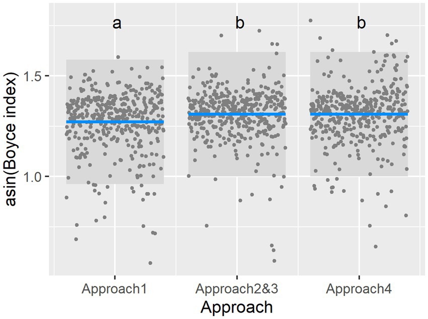
Figure 1. Comparison of models’ predictive performance, as measured by Boyce index, among the different approaches, with Approach 1, which had no anthropogenic data, performing on average worse than other approaches. This is a partial residual graph, with other variables held constant as the approach changes; each point represents a different species. Blue is the predicted mean, and the gray area represents the 95% confidence interval. Columns with the same letter are not significantly different.

The approaches also differed in their predictions as to the distributions of the endemic vertebrates. The approaches that incorporated anthropogenic factors, and eliminated unsuitable habitats and elevation, generally predicted more adverse outcomes for Chinese endemic vertebrates. Specifically, assessing ASH, the overall effect of approach was significant (ANOVA, χ²₂ = 1270.37, p < 0.0001), with the area of suitable habitat largest for Approach 1, intermediate for Approaches 2 and 3, and smallest for Approach 4 (Figure 2A). For LRI, the overall effect of approach was significant (ANOVA, χ²₂ = 1414.19, p < 0.0001), with Approach 2 having the smallest range decrease, Approach 1 slightly larger, Approach 3 being intermediate, and Approach 4 having the highest values (Figure 2C). For CRI, the overall effect of the approach was significant (ANOVA, χ²₂ = 21.54, p < 0.0001), with Approach 4 having lower change of range values than the other approaches (Figure 2B). In all these models, taxa was only significant for ASH (see Supplementary Figure 5B for its effect). SSP was an important explanatory variable for CRI and LRI, and the time period influenced all three models. In general, higher emission SSPs produced more adverse effects than lower emission SPPs, and later periods (i.e., 2081–2100) also produced more extreme effects (Supplementary Table 4).

FIGURE 2

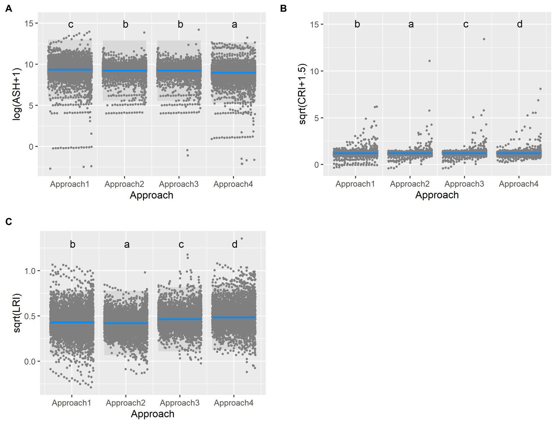
Figure 2. Predictions of the future distributions of Chinese endemic vertebrates varied by approach. Response variables included: (A) Area of suitable habitat (ASH), (B) Loss in Range Index (LRI), and (C) Change in Range Index (CRI). In general, models that incorporated anthropogenic factors (Approaches 2, 3, and 4), and eliminated unsuitable areas from range maps (Approach 4), had more adverse outcomes for Chinese endemic vertebrates.

3.2. Future species’ distributions using Approach 4

3.2.1. Variable importance

As to variable importance, there was a large difference between the 12 explanatory variables in their permutation importance. When looking at mean permutation importance in three classes (climatic, geographic, and anthropogenic), climatic variables were the most influential (Figure 3). The slope was the most important geographic variable, and land use was the most important anthropogenic variable. Results for different taxa are shown in Supplementary Figure 6.

FIGURE 3

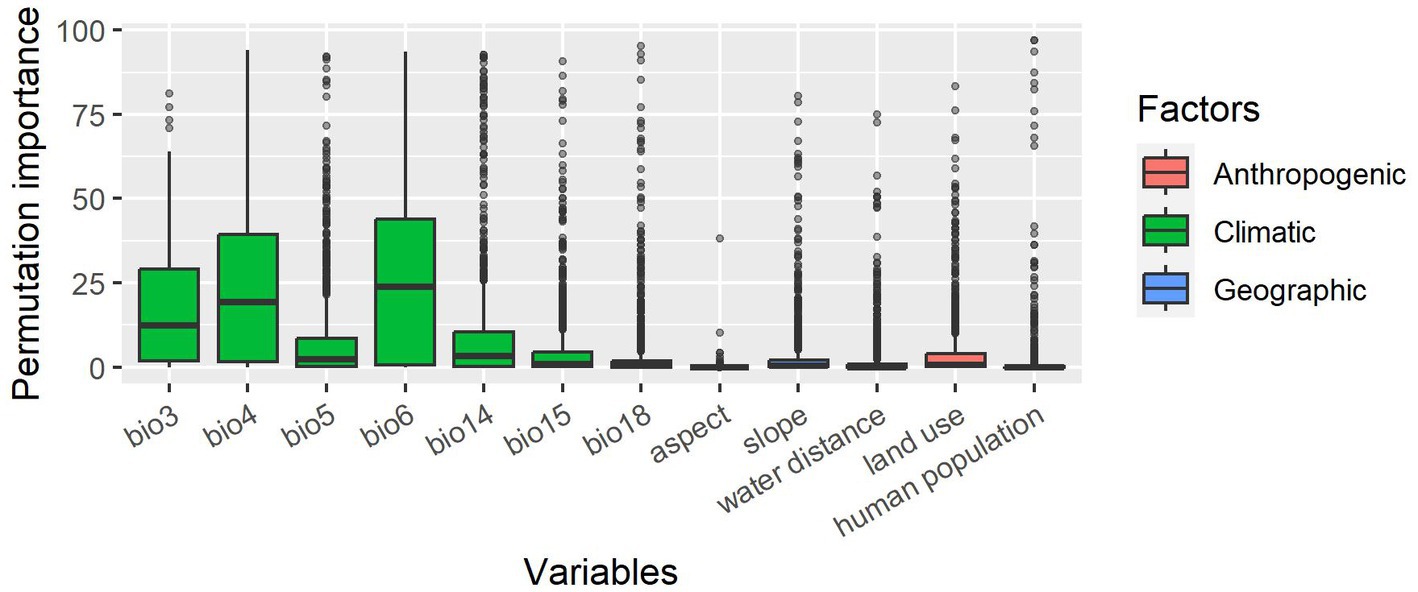
Figure 3. A boxplot of the permutation importance for the 12 explanatory variables in the best models. The variables are classified into three different classes: climatic, geographic, and anthropogenic.

3.2.2. Maps of diversity and descriptions of change over time

A map of the current distributions of the endemic species (Figure 4) shows several major endemic centers for birds and mammals: a large diversity hotspot in mountainous areas around the Sichuan Basin in the north and west of Sichuan, extending into northern Yunnan and eastern Xizang, eastern Qinghai, southern Gansu, southern Shaanxi, northern Guizhou, and Chongqing, as well as another diversity hotspot on the islands of Hainan and Taiwan. In contrast, diversity hotspots for amphibians and reptiles are more diffuse and throughout southern and eastern China.

FIGURE 4

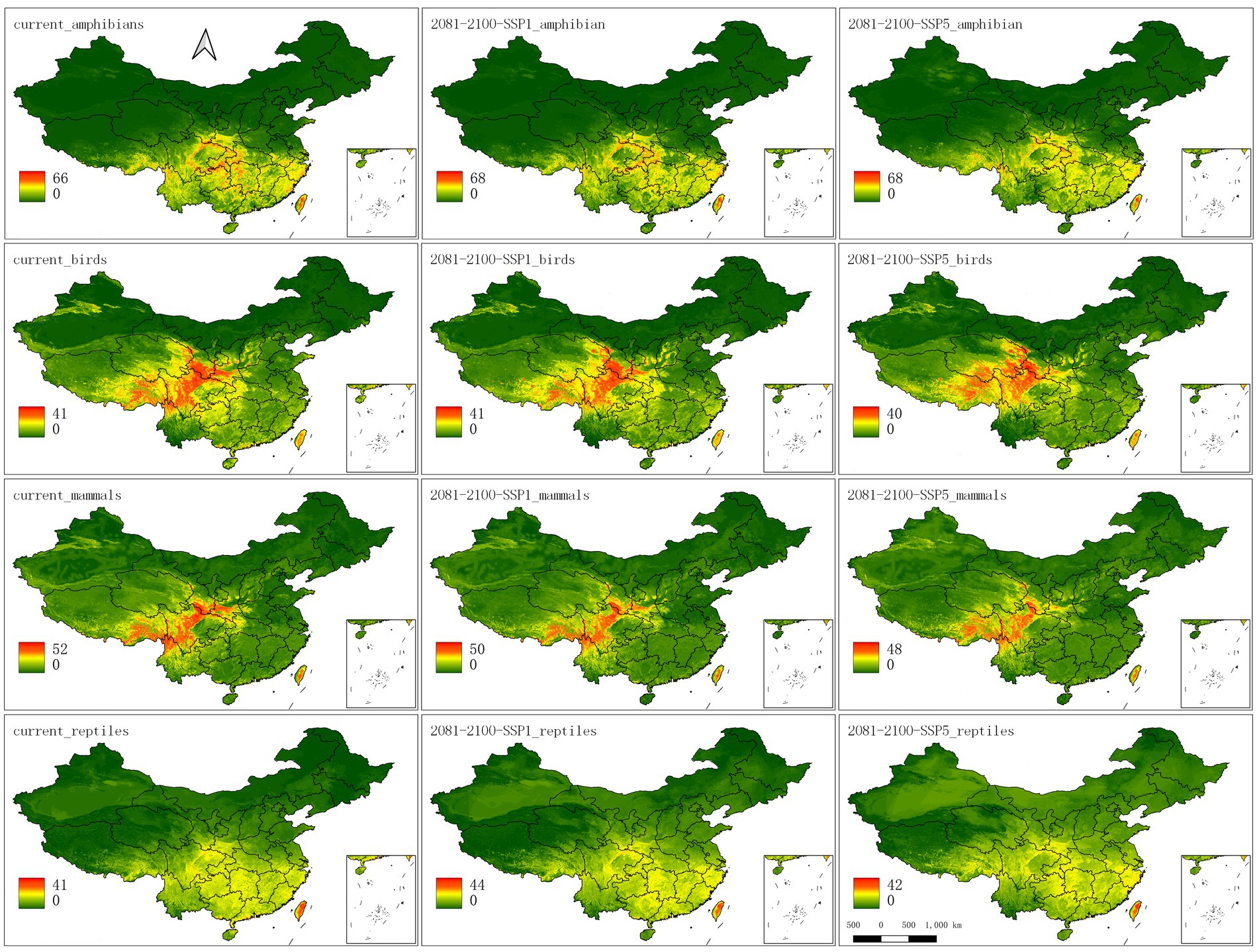
Figure 4. Maps of the current (left), future SSP1 (middle), and SSP5 (right) ranges for each of the four taxa summed across species. The color legend represents the number of species predicted to be present.

In the maps that depict changes in species richness for birds and mammals, there are declines in the current hotspots by 2080–2100, especially for SSP5 (Figures 4, 5). New hotspots emerge for birds and mammals in south to southeast Xizang (Tibet) and southern Qinghai, and even amphibians show movements into this area. Reptiles and mammals show diversity increases across broad swaths of northern China; amphibians show hotspots on the movement map as north as Xinjiang.

FIGURE 5

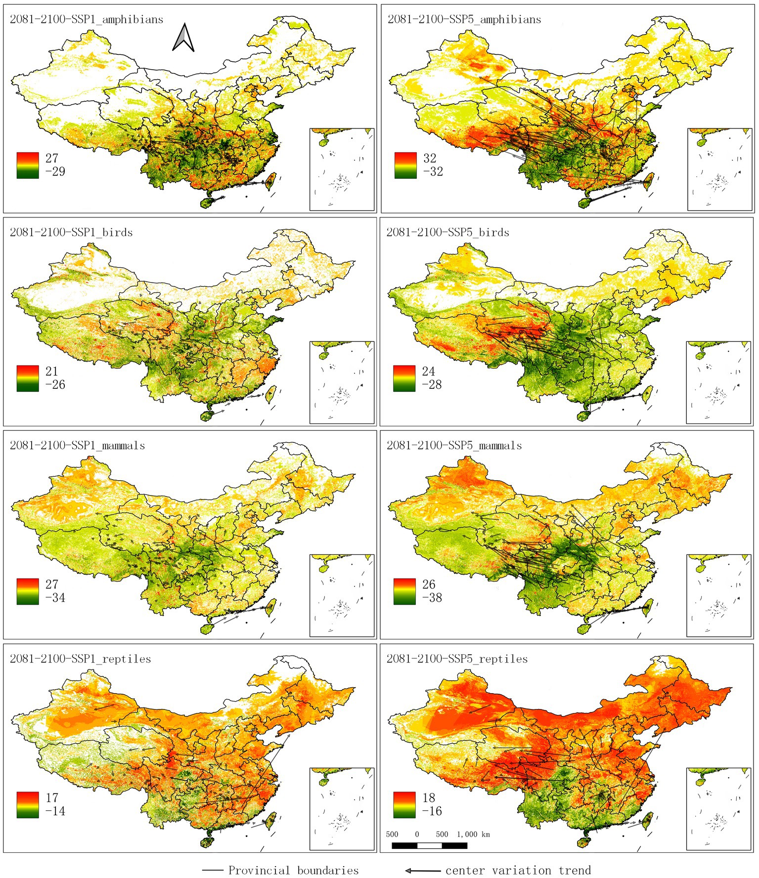
Figure 5. Change maps for the four different taxa and the two different future climate scenarios, SSP1 (left), and SSP5 (right). The arrows point from the current to the future distribution centers. The color legend shows the number of species that shifted in 2080–2100.

The general direction of movement can be analyzed by investigating how the centers of the range for the species change over time (Supplementary Figure 7). Generally, movement tends to be toward the north and to the west (i.e., higher elevations). More extreme climate scenarios show substantial shifts. For example, under SSP5, some species move as much as 15 degrees (around 1,665 km), whereas under SSP1, the movement of all species is almost always less than 5 degrees (around 555 km). At the same time, the animals are moving in terms of elevation (Supplementary Figure 8). In particular, birds and mammals develop under the SSP5 scenario a secondary peak of diversity approximately between 3,500–4,500 m a.s.l.

3.2.3. Analysis of threatened species

The future distributions of species were also influenced by their current threat status, as categorized by the IUCN. Species that are considered threatened by the IUCN face more severe loss of suitable habitat in the future (especially the 2080–2100 period). Specifically, the area of distribution under both the most optimistic SSP1 (ANOVA, χ²₂ = 20.81, p < 0.0001) and the most critical SSP5 (ANOVA, χ²₂ = 12.71, p = 0.0023) scenarios is significantly influenced by the IUCN status (Figure 6). Threatened species have the smallest ASH and highest LCI of all the compared categories. CRI, however, did not show this pattern (being highest for threatened species in SSP1 and not influenced by the IUCN category in SSP5).

FIGURE 6

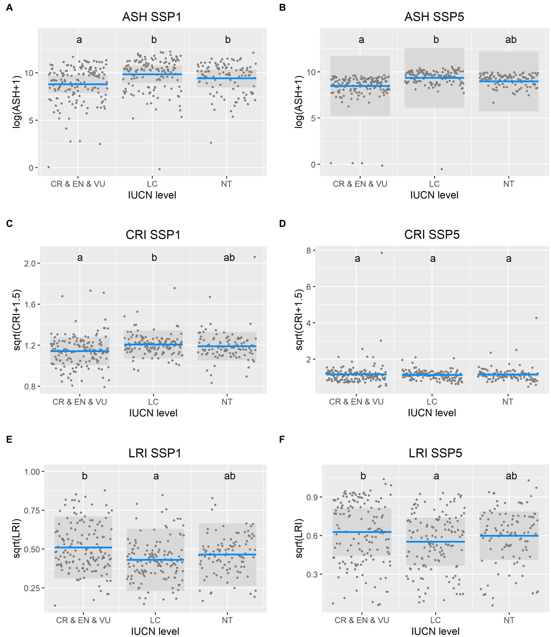
Figure 6. The current threat status of the species was related to their future suitable habitat and how it might change from the current situation. Response variables for the future of Chinese endemic vertebrates in 2081–2100 period are (A) the area of suitable habitat (ASH) in SSP1 scenario and (B) ASH in SSP5 scenario, (C) the change in range index (CRI) in SSP1 scenario and (D) CRI in SSP5 scenario, and (E) the loss of range index (LRI) in SSP1 scenario and (F) LRI in SSP5 scenario. Columns with the same letter are not significantly different.

There are also more species that appear threatened by extinction in the future by more extreme emission scenarios. The number of species facing extinction crises (as measured by less than 20% of the suitable area remaining, or an 80% or more decline of the total range) in the SSP1, SSP2, SSP3, and SSP5 future scenarios was estimated to be 14, 22, 26 and 51, respectively (Supplementary Table 5). For currently threatened species, in particular (CR, EN, and VU), this translated in the SSP1, SSP2, SSP3, and SSP5 scenarios into 5.10, 10.53, 12.81, and 17.59%, respectively, of species (Supplementary Table 5).

4. Discussion

Our results demonstrate that in addition to climatic variables, anthropogenic land-use change and human population densities should also be accounted for when predicting species’ range shifts under global change. Anthropogenic factors have significant influences on species’ survival and ecology and contain a wealth of information that can significantly improve the performance of SDMs. We also found that dynamic anthropogenic factors (i.e., those with estimates into the future) show more dramatic differences in the distribution of species than static ones when projected into the future, with more currently suitable areas becoming unsuitable and narrower distributions predicted. In addition, Approach 4, in which unsuitable areas within the species ranges were removed to reflect the AOH, shows the most potentially adverse results under global change. In terms of China’s endemic vertebrate species, global change may be less harmful to their conservation status than in other countries, because protected areas are larger in the west at higher elevations, providing potential habitat for species to move into. However, it appears that currently threatened species will fare worse, and higher emission scenarios will force more species into extinction in the future, particularly those that are already endangered. This emphasizes the need for China and other countries to immediately reduce greenhouse gas emissions to avoid the worst-case scenarios.

There is an emerging trend to combine static or dynamic anthropogenic factors with climatic factors to construct SDMs (Stanton et al., 2012; Newbold, 2018; Milanesi et al., 2020). Our result suggested that adding anthropogenic variables significantly improved the performance of the modeling procedure. Consistent with previous findings, adding anthropogenic variables containing little redundant information with climatic variables. Land use, in particular, appears to improve modeling outcomes (Martin et al., 2013; Marshall et al., 2018; Della Rocca and Milanesi, 2020). Some earlier studies, for example, Martin et al. (2013), did not find significant differences between using static and dynamic land-use variables. In contrast, in our study, we used a high resolution (2.5 min) and biodiversity-relevant land type classification and found that the dynamic approach showed the potential for more adverse effects (Trisurat et al., 2014; Seaborn et al., 2021; Tang and Zhao, 2022). Overall, land use in China is expected to substantially change between now and 2100, with an expansion of farmland and urban areas, as well as wood harvesting, and in particular, a substantial reduction in temperate and mixed forests (Lai et al., 2016; Dong et al., 2019). Hence it makes sense that dynamic land-use data could contribute to more adverse estimates for Chinese endemic vertebrates.

As for occurrence data, a number of studies have used the species range polygons provided by the IUCN directly, but the shortcomings of the IUCN data have been pointed out for more than a decade (Van Wilgen et al., 2009). Previous research has suggested that IUCN occurrence data should be used with some caution, and that range polygons can exaggerate the species AOH (Ocampo-Peñuela et al., 2016; Brooks et al., 2019; Jung et al., 2020). We found that refining IUCN data into AOH yielded more adverse effects under global change. Since policymakers should plan for the most potentially serious occurrences, this suggests that models using this method are useful.

With regard to the future of Chinese endemic species, we generally obtained consistent results with other studies, where the distribution of species shifts to higher altitudes or higher latitudes under global change (Angert et al., 2011; Hill et al., 2011; Luo et al., 2021). Other studies of Chinese vertebrates, mostly amphibians and birds, have shown that threatened species and endemic species are more vulnerable to climate change (Wu, 2020; Luo et al., 2021). Our results show that species currently listed as threatened by the IUCN might have an increased risk of extinction in the future, which is similar to the results of Li et al. (2013), and requires immediate conservation planning (Li et al., 2013; Zhao et al., 2022). Generally, our results show that while some species’ distribution ranges will increase, a greater number will be severely endangered due to the shrinking of suitable areas and the loss of currently suitable habitats (Li et al., 2013; Wu, 2020). Furthermore, higher emission SSPs aggravate the situation. In response to the already rapidly worsening land degradation and climate change, a number of Chinese policies aim to develop a sustainable future, in particular through the protection and expansion of forests (Chen et al., 2019; Agreement, 2022). Our findings highlight the importance of China and the rest of the world focusing on emission reductions (Fuldauer et al., 2022).

Our study focused on endemic species that are more sensitive to climate change. Future studies could be extended to species with wider ranges. Studies of marine animals (Bayramoglul et al., 2004), invertebrates (Marshall et al., 2018; Liu et al., 2020), plants (Harrison et al., 2006), fungi and microorganisms should also be considered, though the availability of occurrence data for some of those taxa is limited. China is a megadiverse country spanning multiple climatic zones with complex land-use patterns and severe anthropogenic impacts; therefore, it is an important study area in global change research. However, studies from other regions, such as the tropics or boreal regions, are required to generalize results (Louca et al., 2015; Sreekar et al., 2015; Della Rocca and Milanesi, 2020). From the technical perspective, we used a simple buffer to limit the maximum dispersal distance of species, but future studies could add complexities to this framework to better approximate reality (Barve et al., 2011; Lu et al., 2012; Thuiller et al., 2019). For example, many animals may be unable to disperse over marine areas, which may limit species migration to suitable distribution areas. Results for the biodiverse islands of Hainan and Taiwan could be further refined by considerations of this kind.

In conclusion, our findings support the use of an enhanced SDM modeling pathway that incorporates anthropogenic variables and refines IUCN ranges into AOH. Our findings support the recommendation to incorporate dynamic anthropogenic variables, particularly land use, into SDMs (Stanton et al., 2012; Seaborn et al., 2021). High-resolution dynamic anthropogenic variables are now available (De Chazal and Rounsevell, 2009; Chen et al., 2020). We also recommend optimizing the occurrence data for more accurate results that may fully capture potential adverse conditions when using IUCN data, given that high-resolution habitat-type maps and technological advances give us the possibility to estimate the AOH (Jung et al., 2020). The case of Chinese endemic vertebrates demonstrates that climate change can be a threat even in seemingly advantageous situations, such as a large country with more protected areas in the areas where species will move (west and north).

Data availability statement

The original contributions presented in the study are included in the article/Supplementary material, further inquiries can be directed to the corresponding authors.

Author contributions

YD contributed to the conceptualization, investigation, formal analysis, and writing the manuscript. EG contributed to the supervision, conceptualization, investigation, funding acquisition, and improving the manuscript. AD contributed to the data curation, review, and editing the writing. DJ contributed to investigation. AJ contributed to the funding acquisition and investigation. ZZ contributed to the supervision, conceptualization, formal analysis, and improving the manuscript. CM contributed to the supervision, methodology, funding acquisition, and improving the manuscript. All authors read and approved the final manuscript.

Funding

This work was supported by grants from the National Natural Science Foundation of China (Grant number 31870370), and Special Talents Recruitment Grant from Guangxi University.

Acknowledgments

We are grateful to all the researchers and organizations who helped to collect and make publicly available the data used in this study. We also appreciate the comments of two reviewers, which substantially improved the manuscript.

Conflict of interest

The authors declare that the research was conducted in the absence of any commercial or financial relationships that could be construed as a potential conflict of interest.

Publisher’s note

All claims expressed in this article are solely those of the authors and do not necessarily represent those of their affiliated organizations, or those of the publisher, the editors and the reviewers. Any product that may be evaluated in this article, or claim that may be made by its manufacturer, is not guaranteed or endorsed by the publisher.

Supplementary material

The Supplementary material for this article can be found online at: https://www.frontiersin.org/articles/10.3389/fevo.2023.1174495/full#supplementary-material

Footnotes

1. ^http://zoology.especies.cn/

2. ^http://www.earthenv.org/topography

3. ^https://download.geofabrik.de/

4. ^https://data.pnnl.gov/group/nodes/dataset/13192

References

Agreement, T. P. (2022). Effective land management strategies can help climate mitigation in China. Nat. Clim. Change 12, 789–790. doi: 10.1038/s41558-022-01440-3