Intelligent Command Filter Design for Strict Feedback Unmodeled Dynamic MIMO Systems With Applications to Energy Systems

This study presents a command filtered control scheme for multi-input multi-output (MIMO) strict feedback nonlinear unmodeled dynamical systems with its applications to power systems. To deal with dynamic uncertainties, a dynamic signal is introduced, together with radial basis function neural networks (RBFNNs) to overcome the influences of the dynamic uncertainties. Command filters (CFs) are used to prevent the explosion of complexity, where the compensating signals can eliminate the effect of filter errors. Compared with single-input single-output strict feedback nonlinear systems, the method proposed in this study has more suitability. In the end, the simulation experiments are carried out by applying the developed algorithm to power systems, where the simulation results verify the efficacy of the approach proposed.

1 Introduction

In recent years, adaptive control has become a hotspot because of its strong disturbance-rejection property. Related theories, such as model reference control, robust adaptive control, and adaptive dynamic programming (Mukherjee et al., 2017; Yang et al., 2021b; Han and Liu, 2020; Yang et al., 2021d; L’Afflitto, 2018; Yang et al., 2021e), have been applied to many fields, including power systems, wind energy systems, and multi-agent systems (Li et al., 2020; Xu et al., 2018; Wu et al., 2017; Ghaffarzdeh and Mehrizi-Sani, 2020; Zou et al., 2020b; Ghosh and Kamalasadan, 2017; Namazi et al., 2018; Zou et al., 2020a). Moreover, applications of adaptive control on energy systems are also widely reported (Deese and Vermillion, 2021; Quan et al., 2020; Liu et al., 2022; Nascimento Moutinho et al., 2008; Liu et al., 2021). Among them, backstepping is a powerful tool since many energy systems can essentially be modeled as strict feedback systems, which can be analyzed through the backstepping technique.

The main idea of backstepping is to divide the whole system into a series of subsystems so that they can be analyzed individually. In this way, the control design and stability analysis can both be simplified, especially for large-scale systems (Yang et al., 2021a). Meanwhile, for unmodeled dynamical systems, if the unmodeled dynamics are ignored, the disturbance from dynamic uncertainties may result in unbounded evolution. Therefore, the dynamic uncertainties need to be paid enough attention, which is not considered in the aforementioned literatures. Zhao J. et al. (2021) presented a fuzzy adaptive control approach with an observer design for unmodeled dynamical systems. Xia et al. developed an output feedback controldesign with quantized performance for dynamic uncertainties in Xia and Zhang (2018). Wang et al. (2017)investigated nonstrict feedback systems with unmodeled dynamics and dead zones through output feedback-based control methods. Although the aforementioned results can successfully tackle dynamic uncertainties, they are not able to deal with the explosion of complexity and avoid the influences of filter errors.

In the backstepping process, the explosion of complexity often occurs because the virtual control is repeatedly differentiated. Meanwhile, the computational complexity increases significantly, which results in the presented design not being suitable for applications (Yang et al., 2020). To deal with this issue, the dynamic surface control method is proposed (Wang and Huang, 2005). The dynamic surface control method uses first-order filters, where the virtual control is replaced by the filter states in each subsystem (Yang et al., 2021c). In this way, the repeated differentiation issue can be evaded. However, filter errors are introduced simultaneously, which degrades the control precision. Thus, command filters (CFs) are developed (Farrell et al., 2009). Based on the dynamic surface control approach, CFs additionally introduce compensating signals to compensate for the loss caused by filter errors, which further improves the control accuracy compared with the dynamic surface control method. Owing to this advantage, CFs are widely applied to many systems. For example, Zhu et al. (2018)investigated a command filtered robust adaptive neural network (NN) control for strict feedback nonlinear systems with input saturation. Zhao L. et al. (2021)presented an adaptive finite-time tracking control design with CFs. The adaptive fuzzy backstepping control approach of uncertain strict feedback nonlinear systems is developed by Wang et al. (2016). However, the applications of the backstepping technique in energy systems are not taken into consideration in these works. In addition, the systems of interest in these works are single-input single-output systems, which may give conservative results. Therefore, in this study, for multi-input multi-output (MIMO) strict feedback nonlinear unmodeled dynamical systems, a command filtered control method is developed and applied to energy systems.

The contributions of this study are two-fold. First, this study designs an adaptive backstepping control scheme for MIMO strict feedback nonlinear unmodeled dynamical systems with CFs, the compensating signal design and controller design are improved such that they can get higher tracking precision. Second, this study investigates the applications of the presented CF-based adaptive backstepping control approach on power systems, and a MIMO circuit system is used in the simulation experiments to verify the effectiveness of the method developed.

The rest of this article is organized as follows. Section 2 provides the problem formulation and necessary assumptions. In Section 3, the control design is proposed. The stability analysis of the system with the presented design is carried out in Section 4. In Section 5, a voltage source converter-high voltage direct current transmission system is used to verify the efficacy of the proposed method. The conclusion is made in Section 6.

2 Problem Formulation

In this study, the circuit system under consideration is modeled as

$\begin{array}{l}\hfill \begin{array}{cc}\hfill \dot{\varsigma }& =q\left(\varsigma ,X\right),\hfill \\ \hfill {\dot{X}}_i& =F_i\left({\underline{X}}_i\right)+G_i{X}_{i+1}+D_i+{\mathrm{\Delta }}_i\left(\varsigma ,X\right),\hfill \\ \hfill {\dot{X}}_i& =F_n\left(X\right)+G_{n}U+D_n+{\mathrm{\Delta }}_n\left(\varsigma ,X\right),\hfill \\ \hfill y& =X_1,\hfill \end{array}\end{array}(1)$

where $X={\left[X_1\dots X_n\right]}^{\text{T}}\in {\mathbb{R}}^{nm}$, $y\in {\mathbb{R}}^m$, and $U\in {\mathbb{R}}^m$ are the system state, output, and the control input, respectively. $F_i(\cdot ):{\mathbb{R}}^{im}\to {\mathbb{R}}^m$ is a known continuous function, $q(\cdot ,\cdot ):\mathbb{R}\times {\mathbb{R}}^{nm}\to \mathbb{R}$ is an unknown continuous function, G_i ≠ 0 is a known constant, $D_i\in {\mathbb{R}}^m$ is an unknown constant vector, ${\underline{X}}_i={\left[X_1,\cdots ,X_i\right]}^{\text{T}}\in {\mathbb{R}}^{im}$, $\varsigma \in \mathbb{R}$ is the unmeasured portion of the state, and ${\mathrm{\Delta }}_i\in {\mathbb{R}}^m$ is the unmodeled dynamics.

In this study, the following assumptions are needed.

Assumption 1. Jiang and Praly (1998): The dynamic uncertainty Δ_i in Eq. 1 is assumed to satisfy

$‖{\mathrm{\Delta }}_i\left(\varsigma ,X\right)‖\le {\varphi }_{i1}\left(‖{\underline{X}}_i‖\right)+{\varphi }_{i2}\left(‖\varsigma ‖\right),i=1,\dots ,n(2)$

with unknown smooth functions ${\varphi }_{i1}\left(\cdot \right):{\mathbb{R}}_0^{+}\to {\mathbb{R}}_0^{+}$ and ${\varphi }_{i2}\left(\cdot \right):{\mathbb{R}}_0^{+}\to {\mathbb{R}}_0^{+}$. In addition, ${\varphi }_{i2}\left(\cdot \right)$ is assumed to be strictly increasing.

Assumption 2. Jiang and Praly (1998): There exists an input-to-state practically stable Lyapunov function $V_{\varsigma }\left(\varsigma \right)$ for $\dot{\varsigma }=q\left(\varsigma ,X\right)$ in Eq. 1 such that

$\begin{array}{l}\hfill \begin{array}{cc}\hfill {\omega }_1\left(‖\varsigma ‖\right)& \le V_{\varsigma }\left(\varsigma \right)\le {\omega }_2\left(‖\varsigma ‖\right),\hfill \\ \hfill \frac{\partial V_{\varsigma }}{\partial \varsigma }q\left(\varsigma ,X\right)& \le -c_0{V}_{\varsigma }\left(\varsigma \right)+\mathit{\vartheta }\left(‖X_1‖\right)+d_0,\hfill \end{array}\end{array}(3)$

with ω₁ and ω₂ belonging to class ${\mathcal{K}}_{\infty }$ functions, $\vartheta \left(\cdot \right):{\mathbb{R}}_0^{+}\to {\mathbb{R}}_0^{+}$, and c₀ and d₀ being positive constants.To deal with the dynamic uncertainty, a dynamic signal is designed with the following dynamics,

$\dot{r}=-\bar{c}r+\bar{\vartheta }\left(‖X_1‖\right)+d_0,r\left(0\right)=r_0,(4)$

where $\bar{\vartheta }\left(X_1\right)\ge \vartheta \left(‖X_1‖\right)$, $\bar{c}\in \left(0,c_0\right)$, and c₀ > 0 and r₀ are constants.

Lemma 1. Hardy et al. (1952): For any ξ₀ > 0, one has

$0\le ‖{\xi }_0‖-{\xi }_0\tanh \left(\frac{{\xi }_0}{\chi }\right)\le 0.2785\chi ,$

where χ > 0 is a constant.

Lemma 2. Jiang and Praly (1998):For the unmeasured partial state $\varsigma \left(t\right)$ with initial state ς₀, $V_{\varsigma }\left(\varsigma \right)$ given in Assumption 2, the dynamic signal r(t) in Eq. 4, and all t ≥ 0, there is a non-negative function $B\left(t\right)$ such that

$V_{\varsigma }\left(\varsigma \right)\le r\left(t\right)+\mathrm{\Phi }\left(t\right).(5)$

In addition, there is a limited time $T_0=T_0\left({\bar{c}}_0,r_0,{\varsigma }_0\right)$ such that $\mathrm{\Phi }\left(t\right)=0$ for all t ≥  T₀.With no loss of generality, choose $\bar{\mathrm{\Theta }}\left(X_1\right)$ as $\bar{\mathrm{\Theta }}\left(X_1\right)=X_1^2\mathrm{\Theta }\left(X_1^2\right)$. Accordingly, the dynamic signal r(t) is designed as

$\dot{r}=-\bar{c}r+X_1^2\mathrm{\Theta }\left(X_1^2\right)+d_0,r\left(0\right)=r_0.(6)$

The control objective of this study can be formulated as follows.Control Objective: Consider the reference output X_d satisfying $\left\{X_d,,,{\dot{X}}_d,,,{\ddot{X}}_d\right\}$ are bounded. Under Assumptions 1–2, design a neuro-adaptive controller for the system (1), such that,

1. the system output X₁ can track the reference X_d asymptotically, and

2. all signals in the closed-loop system keep bounded.

3 Neuro-Adaptive Controller Design

First, the tracking errors E_i, filter errors Z_i, and the compensated tracking errors Λ_i are defined for each subsystem as

$\begin{array}{l}\hfill \begin{array}{cc}\hfill E_i& =X_i-A_{i-1},i=\mathrm{1,2,3},\hfill \\ \hfill Z_i& =A_i-S_i,i=\mathrm{1,2},\hfill \\ \hfill {\mathrm{\Lambda }}_i& =E_i-B_i,i=\mathrm{1,2,3},\hfill \end{array}\end{array}(7)$

where A_i is the filter state, A₀ = X_d, S_i is the virtual control, and B_i is the compensating signal.

For the subsequent design and analysis, denote ${\mathrm{\Theta }}_i={‖W_i^{*}‖}^i,i=1,\dots ,n$ with $W_i^{*}$ being the ideal weight vector of the RBFNNs. In addition, denote ${\widehat{\mathrm{\Theta }}}_i\left(t\right)$ as the estimation of Θ_i with an estimation error ${\tilde{\mathrm{\Theta }}}_i\left(t\right)={\mathrm{\Theta }}_i-{\widehat{\mathrm{\Theta }}}_i\left(t\right)$.

3.1 Adaptive Backstepping Design

3.1.1 Step 1

Based on Eqs 1, 7, taking a derivative of E₁ yields

$\begin{array}{cc}{\dot{E}}_1=\hfill & \hfill F_1\left(X_1\right)+G_1{X}_2+D_1+{\mathrm{\Delta }}_1-{\dot{X}}_d\\ \hfill & \hfill =F_1\left(X_1\right)+G_1{E}_2+G_1{S}_1+G_1{Z}_1+D_1+{\mathrm{\Delta }}_1-{\dot{X}}_d.\end{array}(8)$

For the first subsystem, the virtual control S₁ is designed as

$S_1=\frac{1}{G_1}\left(-F_1-K_1{E}_1-\frac{{\widehat{\mathrm{\Theta }}}_1}{2{\eta }_1}{\mathrm{\Lambda }}_1{\phi }_1^{\text{T}}{\phi }_1+{\dot{X}}_d\right),(9)$

with $K_1=\mathrm{diag}\left\{K_{11},\cdots ,K_{1m}\right\}$ is a positive definite matrix, and η₁ > 0. To avoid repeated differentiation of the virtual control, a CF is designed as

${\dot{A}}_1=\frac{S_1-A_1}{{\tau }_1},A_1\left(0\right)=S_1\left(0\right),(10)$

with a positive constant τ₁. To eliminate the effect of filter errors, the compensating signal is developed as

${\dot{B}}_1=-K_1{B}_1+G_1{B}_2+G_1{Z}_1,B_1\left(0\right)=0.(11)$

To compensate for the unknown dynamics, the adaptive law for Θ₁ is presented as

${\dot{\widehat{\mathrm{\Theta }}}}_1=\frac{1}{2{\eta }_1}{\mathrm{\Lambda }}_1^{\text{T}}{\mathrm{\Lambda }}_1{\phi }_1^{\text{T}}{\phi }_1-{\gamma }_1{\widehat{\mathrm{\Theta }}}_1,{\widehat{\mathrm{\Theta }}}_1\left(0\right)=0,(12)$

where γ₁ > 0 is a constant.

3.1.2 Step $\mathit{i}\left(\mathbf{2}\mathbf{\le }\mathit{i}\mathbf{\le }\mathit{n}\mathbf{-}\mathbf{1}\right)$

From Eqs 1, 7, differentiating E_i leads to

$\begin{array}{cc}{\dot{E}}_i\hfill & \hfill =F_i+G_i{X}_{i+1}+D_i+{\mathrm{\Delta }}_i-{\dot{A}}_{i-1}\\ \hfill & \hfill =F_i+G_i{E}_{i+1}+G_i{S}_i+G_i{Z}_i+D_i+{\mathrm{\Delta }}_i-{\dot{A}}_{i-1}.\end{array}(13)$

The virtual control design S_i is developed as

$S_i=\frac{1}{G_i}\left(-F_i-G_{i-1}{E}_{i-1}-K_i{E}_i-\frac{{\widehat{\mathrm{\Theta }}}_i}{2{\eta }_i}{\mathrm{\Lambda }}_i{\phi }_i^{\text{T}}{\phi }_i+{\dot{A}}_{i-1}\right),(14)$

where $K_i=\mathrm{diag}\left\{K_{i1},\cdots ,K_{im}\right\}$ is a positive definite matrix, and η_i > 0. To obviate repeated differentiation of the virtual control S_i, a CF is given as

${\dot{A}}_i=\frac{S_i-A_i}{{\tau }_i},A_i\left(0\right)=S_i\left(0\right),(15)$

with a positive design parameter τ_i. To diminish the influences of filter errors, the compensating signal is proposed as

${\dot{B}}_i=-G_{i-1}{B}_{i-1}-K_i{B}_i+G_i{B}_{i+1}+G_i{Z}_i,B_i\left(0\right)=0.(16)$

To deal with the parameter estimation, the adaptive law to estimate Θ_i is designed as

${\dot{\widehat{\mathrm{\Theta }}}}_i=\frac{1}{2{\eta }_i}{\mathrm{\Lambda }}_i^{\text{T}}{\mathrm{\Lambda }}_i{\phi }_i^{\text{T}}{\phi }_i-{\gamma }_i{\widehat{\mathrm{\Theta }}}_i,{\widehat{\mathrm{\Theta }}}_i\left(0\right)=0,(17)$

with a constant γ_i > 0.

3.1.3 Step n

According to Eqs 1, 7, the differentiation of E_n can be transformed as

${\dot{E}}_n=F_n+G_{n}U+D_n+{\mathrm{\Delta }}_n-{\dot{A}}_{n-1}.(18)$

The controller design is given as

$U=\frac{1}{G_n}\left(-F_n-G_{n-1}{E}_{n-1}-K_n{E}_n-\frac{{\widehat{\mathrm{\Theta }}}_n}{2{\eta }_n}{\mathrm{\Lambda }}_n{\phi }_n^{\text{T}}{\phi }_n+{\dot{A}}_{n-1}\right),(19)$

with design parameters $K_n=\mathrm{diag}\left\{K_{n1},\cdots ,K_{nm}\right\}$ is a positive definite matrix, and η_n > 0. The compensating signal for this step is presented as

${\dot{B}}_n=-G_{n-1}{B}_{n-1}-K_n{B}_n,B_n\left(0\right)=0.(20)$

The adaptive law is developed as

${\dot{\widehat{\mathrm{\Theta }}}}_n=\frac{1}{2{\eta }_n}{\mathrm{\Lambda }}_n^{\text{T}}{\mathrm{\Lambda }}_n{\phi }_n^{\text{T}}{\phi }_n-{\gamma }_n{\widehat{\mathrm{\Theta }}}_n,{\widehat{\mathrm{\Theta }}}_n\left(0\right)=0,(21)$

where γ_n > 0 is a constant.

4 Stability Analysis

In this section, we analyze the stability of the closed-loop system (Eq. 1) with the presented design of the virtual control (Eqs 9, 14), controller (Eq. 19), adaptive laws (Eqs 12, 17, 21), CFs (Eq. 10) and (15), and compensating signals (Eqs 11, 16, 20).

4.1 Step 1

Inserting Eq. 9 into Eq. 8, we obtain

${\dot{E}}_1=-K_1{E}_1+G_1{E}_2+G_1{Z}_1-\frac{{\widehat{\mathrm{\Theta }}}_1}{2{\eta }_1}{\mathrm{\Lambda }}_1{\phi }_1^{\text{T}}{\phi }_1+D_1+{\mathrm{\Delta }}_1.(22)$

From the aforementioned equation and Eq. 11, one has

${\dot{\mathrm{\Lambda }}}_1=-K_1{\mathrm{\Lambda }}_1+G_1{\mathrm{\Lambda }}_2-\frac{{\widehat{\mathrm{\Theta }}}_1}{2{\eta }_1}{\mathrm{\Lambda }}_1{\phi }_1^{\text{T}}{\phi }_1+D_1+{\mathrm{\Delta }}_1.(23)$

The Lyapunov function is defined as $V_1\left({\mathrm{\Lambda }}_1,{\tilde{\mathrm{\Theta }}}_1\right)=\frac{1}{2}{\mathrm{\Lambda }}_1^{\text{T}}{\mathrm{\Lambda }}_1+\frac{1}{2}{\tilde{\mathrm{\Theta }}}_1^{\text{T}}{\tilde{\mathrm{\Theta }}}_1$. From Assumption 1, the term ${\mathrm{\Lambda }}_1^{\text{T}}{\mathrm{\Delta }}_1$ satisfies

${\mathrm{\Lambda }}_1^{\text{T}}{\mathrm{\Delta }}_1\le ‖{\mathrm{\Lambda }}_1‖{\varphi }_{11}\left(‖X_1‖\right)+‖{\mathrm{\Lambda }}_1‖{\varphi }_{12}\left(‖\varsigma ‖\right).(24)$

For the term $‖{\mathrm{\Lambda }}_1‖{\varphi }_{11}\left(‖X_1‖\right)$ in the aforementioned equation, based on Lemma 1, one has

$‖{\mathrm{\Lambda }}_1‖{\varphi }_{11}\left(X_1,{\mathrm{\Lambda }}_1\right)\le {\mathrm{\Lambda }}_1^{\text{T}}{\widehat{\varphi }}_{11}\left(‖X_1‖\right)+{{\epsilon }^{\prime }}_{11},{{\epsilon }^{\prime }}_{11}=0.2785{\epsilon }_{11},(25)$

with ${\epsilon }_{11}^{\prime }$ and ɛ₁₁ being positive constants and

${\widehat{\varphi }}_{11}\left(X_1,{\mathrm{\Lambda }}_1\right)={\varphi }_{11}\left(‖X_1‖\right)\tanh \left(\frac{{\mathrm{\Lambda }}_1^{\text{T}}{\varphi }_{11}\left(‖X_1‖\right)}{{\epsilon }_{11}}\right).$

Consider the term $‖{\mathrm{\Lambda }}_1‖{\varphi }_{12}\left(‖\varsigma ‖\right)$ in Eq. 24, according to Lemma 2, we have

$‖{\mathrm{\Lambda }}_1‖{\varphi }_{12}\left(‖\varsigma ‖\right)\le ‖{\mathrm{\Lambda }}_1‖{\varphi }_{12}\left({\omega }_1^{-1}\left(r+\mathrm{\Phi }\right)\right).(26)$

It is to be noted that ϕ₁₂(⋅) is strictly increasing and non-negative from Assumption 1, together with the fact that $r+\mathrm{\Phi }\le \max \left\{2r,2\mathrm{\Phi }\right\}$, one has

$\begin{array}{ll}\hfill ‖{\mathrm{\Lambda }}_1‖{\varphi }_{12}\left({\omega }_1^{-1}\left(r+\mathrm{\Phi }\right)\right)& \le ‖{\mathrm{\Lambda }}_1‖{\varphi }_{12}\left({\omega }_1^{-1}\left(2r\right)\right)\hfill \\ \hfill & +‖{\mathrm{\Lambda }}_1‖{\varphi }_{12}\left({\omega }_1^{-1}\left(2\mathrm{\Phi }\right)\right).\hfill \end{array}(27)$

From Lemma 1, we can obtain

$‖{\mathrm{\Lambda }}_1‖{\varphi }_{12}\left({\omega }_1^{-1}\left(2r\right)\right)\le {\mathrm{\Lambda }}_1^{\text{T}}{\widehat{\varphi }}_{12}\left({\mathrm{\Lambda }}_1,r\right)+{{\epsilon }^{\prime }}_{12},{{\epsilon }^{\prime }}_{12}=0.2785{\epsilon }_{12},(28)$

where ${\epsilon }_{12}^{\prime }$ and ε₁₂ are positive constants, and

${\widehat{\varphi }}_{12}\left({\mathrm{\Lambda }}_1,r\right){\varphi }_{12}\left({\omega }_1^{-1}\left(2r\right)\right)\tanh \left(\frac{{\mathrm{\Lambda }}_1{\varphi }_{12}\left({\omega }_1^{-1}\left(2r\right)\right)}{{\epsilon }_{12}}\right),$

$‖{\mathrm{\Lambda }}_1‖{\varphi }_{12}‖\left({\omega }_1^{-1}\left(2\mathrm{\Phi }\right)\right)‖\le \frac{1}{4}{\mathrm{\Lambda }}_1^{\text{T}}{\mathrm{\Lambda }}_1+d_1\left(t\right),(29)$

where $d_1\left(t\right)={\varphi }_{12}^2\left({\omega }_1^{-1}\left(2\mathrm{\Phi }\left(t\right)\right)\right)$. From Eqs 23–29, the derivative of V₁ can be expressed as

$\begin{array}{ll}\hfill {\dot{V}}_1& ={\mathrm{\Lambda }}_1^{\text{T}}\left(-K_1{\mathrm{\Lambda }}_1+G_1{\mathrm{\Lambda }}_2-\frac{{\widehat{\mathrm{\Theta }}}_1}{2{\eta }_1}{\mathrm{\Lambda }}_1{\phi }_1^{\text{T}}{\phi }_1+D_1+{\mathrm{\Delta }}_1\right)-{\tilde{\mathrm{\Theta }}}_1^{\text{T}}{\dot{\widehat{\mathrm{\Theta }}}}_1\hfill \\ \hfill & \le -{\mathrm{\Lambda }}_1^{\text{T}}{K}_1{\mathrm{\Lambda }}_1-\frac{{\widehat{\mathrm{\Theta }}}_1}{2{\eta }_1}{\mathrm{\Lambda }}_1^{\text{T}}{\mathrm{\Lambda }}_1{\phi }_1^{\text{T}}{\phi }_1+G_1{\mathrm{\Lambda }}_1^{\text{T}}{\mathrm{\Lambda }}_2+\frac{1}{2}{\mathrm{\Lambda }}_1^{\text{T}}{\mathrm{\Lambda }}_1\hfill \\ \hfill & +\frac{1}{2}{D}_1^{\text{T}}{D}_1-{\tilde{\mathrm{\Theta }}}_1^{\text{T}}{\dot{\widehat{\mathrm{\Theta }}}}_1+{\mathrm{\Lambda }}_1^{\text{T}}{\widehat{\varphi }}_{11}\left(x_1,{\mathrm{\Lambda }}_1\right)+{{\epsilon }^{\prime }}_{11}+{\mathrm{\Lambda }}_1^{\text{T}}{\widehat{\varphi }}_{12}\left({\mathrm{\Lambda }}_1,r\right)\hfill \\ \hfill & +{{\epsilon }^{\prime }}_{12}+\frac{1}{4}{\mathrm{\Lambda }}_1^{\text{T}}{\mathrm{\Lambda }}_1+d_1\left(t\right).\hfill \end{array}(30)$

Using RBFNNs satisfies

$\begin{array}{ll}\hfill {\dot{V}}_1& \le -{\mathrm{\Lambda }}_1^{\text{T}}{K}_1{\mathrm{\Lambda }}_1-\frac{{\widehat{\mathrm{\Theta }}}_1}{2{\eta }_1}{\mathrm{\Lambda }}_1^{\text{T}}{\mathrm{\Lambda }}_1{\phi }_1^{\text{T}}{\phi }_1+G_1{\mathrm{\Lambda }}_1^{\text{T}}{\mathrm{\Lambda }}_2\hfill \\ \hfill & +{\mathrm{\Lambda }}_1{H}_1\left(Y_1\right)+\frac{1}{2}{D}_1^{\text{T}}{D}_1+{{\epsilon }^{\prime }}_{11}+{{\epsilon }^{\prime }}_{12}+d_1\left(t\right)-{\tilde{\mathrm{\Theta }}}_1^{\text{T}}{\dot{\widehat{\mathrm{\Theta }}}}_1,\hfill \end{array}(31)$

where $H_1\left(Y_1\right)={\widehat{\varphi }}_{11}\left(x_1,{\mathrm{\Lambda }}_1\right)+{\widehat{\varphi }}_{12}\left({\mathrm{\Lambda }}_1,r\right)+\frac{3}{4}{\mathrm{\Lambda }}_1,Y_1={\left[X_1,{\mathrm{\Lambda }}_1,r\right]}^{\text{T}}$. It is to be noted that $H_1\left(Y_1\right)$ is an unknown function. Then, according to the universal approximation theory, the unknown function $H_1\left(Y_1\right)$ can be approximated by the RBFNNs in the following form,

${\widehat{H}}_1\left(\left.Y_1\right|W_1^{*}\right)=W_1^{*T}{\phi }_1\left(Y_1\right),(32)$

with $W_1^{*}$ being the ideal weight vector defined as

$W_1^{*}=\underset{W_1\in {\mathrm{\Omega }}_{W_1}}{\arg \min }\left[\underset{Y_1\in {\mathrm{\Omega }}_{Y_1}}{\sup }‖{\widehat{H}}_1\left(\left.Y_1\right|W_1\right)-H_1\left(Y_1\right)‖\right],$

where ${\mathrm{\Omega }}_{W_1}$ and ${\mathrm{\Omega }}_{Y_1}$ are compact regions for W₁ and Y₁, respectively. The corresponding approximation error ${\epsilon }_1^{*}$ is defined as

${\epsilon }_1^{*}=H_1\left(Y_1\right)-{\widehat{H}}_1\left(\left.Y_1\right|W_1^{*}\right),$

with $‖{\epsilon }_1^{*}‖\le {\epsilon }_1$ and a positive constant ε₁.

Based on the definition of Θ₁, combining with Young’s inequality, we have

${\mathrm{\Lambda }}_1^{\text{T}}{H}_1\left(Y_1\right)\le \frac{{\mathrm{\Theta }}_1}{2{\eta }_1}{\mathrm{\Lambda }}_1^{\text{T}}{\mathrm{\Lambda }}_1{\phi }_1^{\text{T}}{\phi }_1+\frac{{\eta }_1}{2}+\frac{1}{2}\left({\mathrm{\Lambda }}_1^{\text{T}}{\mathrm{\Lambda }}_1+{\epsilon }_1^2\right).(33)$

Inserting Eq. 33 into Eq. 31 yields

$\begin{array}{cc}{\dot{V}}_1\le \hfill & \hfill -{\mathrm{\Lambda }}_1^{\text{T}}{K}_1{\mathrm{\Lambda }}_1-\frac{{\mathrm{\Lambda }}_1{\mathrm{\Lambda }}_i}{L_i}+\frac{{\tilde{\mathrm{\Theta }}}_1}{2{\eta }_1}{\mathrm{\Lambda }}_1^{\text{T}}{\mathrm{\Lambda }}_1{\phi }_1^{\text{T}}{\phi }_1+\frac{{\eta }_1}{2}\\ \hfill & \hfill +\frac{1}{2}\left({\mathrm{\Lambda }}_1^{\text{T}}{\mathrm{\Lambda }}_1+{\epsilon }_1^2\right)+{\epsilon }_{11}^{\prime }+{\epsilon }_{12}^{\prime }+d_1\left(t\right)-{\tilde{\mathrm{\Theta }}}_1^{\text{T}}{\dot{\widehat{\mathrm{\Theta }}}}_1.\end{array}(34)$

4.2 Step $\mathit{i}\left(\mathbf{2}\mathbf{\le }\mathit{i}\mathbf{\le }\mathit{n}\mathbf{-}\mathbf{1}\right)$

Inserting the virtual control design Eq. 14 into Eq. 13, we have

${\dot{E}}_i=-G_{i-1}{E}_{i-1}-K_i{E}_i+G_i{E}_{i+1}+G_i{Z}_i-\frac{{\widehat{\mathrm{\Theta }}}_i}{2{\eta }_i}{\mathrm{\Lambda }}_i{\phi }_i^{\text{T}}{\phi }_i+D_i+{\mathrm{\Delta }}_i.(35)$

On the basis of Eq. 16 and the aforementioned equation, one can obtain

${\dot{\mathrm{\Lambda }}}_i=-G_{i-1}{\mathrm{\Lambda }}_{i-1}-K_i{\mathrm{\Lambda }}_i+G_i{\mathrm{\Lambda }}_{i+1}-\frac{{\widehat{\mathrm{\Theta }}}_i}{2{\eta }_i}{\mathrm{\Lambda }}_i{\phi }_i^{\text{T}}{\phi }_i+D_i+{\mathrm{\Delta }}_i.(36)$

To analyze the stability of the i-th subsystem through the Lyapunov theory, define the Lyapunov function for Λ_i and ${\tilde{\mathrm{\Theta }}}_i$ as $V_i\left({\mathrm{\Lambda }}_i,{\tilde{\mathrm{\Theta }}}_i\right)=\frac{1}{2}{\mathrm{\Lambda }}_i^{\text{T}}{\mathrm{\Lambda }}_i+\frac{1}{2}{\tilde{\mathrm{\Theta }}}_i^{\text{T}}{\tilde{\mathrm{\Theta }}}_i$. Based on Assumption 1, the term ${\mathrm{\Lambda }}_i^{\text{T}}{\mathrm{\Delta }}_i$ satisfies

${\mathrm{\Lambda }}_i^{\text{T}}{\mathrm{\Delta }}_i\le ‖{\mathrm{\Lambda }}_i‖{\varphi }_{i1}\left(‖{\underline{X}}_i‖\right)+‖{\mathrm{\Lambda }}_i‖{\varphi }_{i2}\left(‖\varsigma ‖\right).(37)$

Consider the term $‖{\mathrm{\Lambda }}_i‖{\varphi }_{i1}\left(‖{\underline{X}}_i‖\right)$ in Eq. 37, on account of Lemma 1, one has

$‖{\mathrm{\Lambda }}_i‖{\varphi }_{i1}\left(‖{\underline{X}}_i‖\right)\le {\mathrm{\Lambda }}_i^{\text{T}}{\widehat{\varphi }}_{i1}\left({\underline{X}}_i,{\mathrm{\Lambda }}_i\right)+{{\epsilon }^{\prime }}_{i1},{{\epsilon }^{\prime }}_{i1}=0.2785{\epsilon }_{i1},(38)$

with ${{\epsilon }^{\prime }}_{i1}>0$, ɛ_i1 > 0, and

${\widehat{\varphi }}_{i1}\left({\underline{X}}_i,{\mathrm{\Lambda }}_i\right)={\varphi }_{i1}\left(‖{\underline{X}}_i‖\right)\tanh \left(\frac{{\mathrm{\Lambda }}_i{\varphi }_{i1}\left(‖{\underline{X}}_i‖\right)}{{\epsilon }_{i1}}\right).$

For the term $‖{\mathrm{\Lambda }}_i‖{\varphi }_{i2}\left(‖\varsigma ‖\right)$ in (37), according to Lemma 2, we can obtain

$‖{\mathrm{\Lambda }}_i‖{\varphi }_{i2}\left(‖\varsigma ‖\right)\le ‖{\mathrm{\Lambda }}_i‖{\varphi }_{i2}\left({\omega }_1^{-1}\left(r+\mathrm{\Phi }\right)\right).(39)$

Since ϕ_i2 is strictly increasing and non-negative from Assumption 1, based on the fact $r+\mathrm{\Phi }\le \max \left\{2r,2\mathrm{\Phi }\right\}$, one has

$\begin{array}{ll}\hfill ‖{\mathrm{\Lambda }}_i‖{\varphi }_{i2}\left({\omega }_1^{-1}\left(r+\mathrm{\Phi }\right)\right)& \le ‖{\mathrm{\Lambda }}_i‖{\varphi }_{i2}\left({\omega }_1^{-1}\left(2r\right)\right)\hfill \\ \hfill & +‖{\mathrm{\Lambda }}_i‖{\varphi }_{i2}\left({\omega }_1^{-1}\left(2\mathrm{\Phi }\right)\right).\hfill \end{array}(40)$

On the basis of Lemma 1, we can obtain

$‖{\mathrm{\Lambda }}_i‖{\varphi }_{i2}\left({\omega }_1^{-1}\left(2r\right)\right)\le {\mathrm{\Lambda }}_i^{\text{T}}{\widehat{\varphi }}_{i2}\left({\mathrm{\Lambda }}_i,r\right)+{{\epsilon }^{\prime }}_{i2},{{\epsilon }^{\prime }}_{i2}=0.2785{\epsilon }_{i2},(41)$

with ${{\epsilon }^{\prime }}_{i2}>0$, ɛ_i2 > 0, and

${\widehat{\varphi }}_{i2}\left({\mathrm{\Lambda }}_i,r\right)={\varphi }_{i2}\left({\omega }_1^{-1}\left(2r\right)\right)\tanh \left(\frac{{\mathrm{\Lambda }}_i{\varphi }_{i2}\left({\omega }_1^{-1}\left(2r\right)\right)}{{\epsilon }_{i2}}\right).$

Using Young’s inequality, we have

$‖{\mathrm{\Lambda }}_i‖{\varphi }_{i2}\left({\omega }_1^{-1}\left(2\mathrm{\Phi }\right)\right)\le \frac{1}{4}{\mathrm{\Lambda }}_i^{\text{T}}{\mathrm{\Lambda }}_i+d_i\left(t\right),(42)$

where $d_i\left(t\right)={\varphi }_{i2}^2\left({\omega }_1^{-1}\left(2\mathrm{\Phi }\left(t\right)\right)\right)$.

From Eqs 36–42, the derivative of V_i becomes

$\begin{array}{ll}\hfill {\dot{V}}_i& ={\mathrm{\Lambda }}_i\left(-G_{i-1}{\mathrm{\Lambda }}_{i-1}-K_i{\mathrm{\Lambda }}_i+G_i{\mathrm{\Lambda }}_{i+1}\right.\hfill \\ \hfill & \left.-\frac{{\widehat{\mathrm{\Theta }}}_i}{2{\eta }_i}{\mathrm{\Lambda }}_i{\phi }_i^{\text{T}}{\phi }_i+D_i+{\mathrm{\Delta }}_i\right)-{\tilde{\mathrm{\Theta }}}_i^{\text{T}}{\dot{\widehat{\mathrm{\Theta }}}}_i\hfill \\ \hfill & \le -G_{i-1}{\mathrm{\Lambda }}_{i-1}^{\text{T}}{\mathrm{\Lambda }}_i-{\mathrm{\Lambda }}_i^{\text{T}}{K}_i{\mathrm{\Lambda }}_i+G_i{\mathrm{\Lambda }}_i^{\text{T}}{\mathrm{\Lambda }}_{i+1}-\frac{{\widehat{\mathrm{\Theta }}}_i}{2{\eta }_i}{\mathrm{\Lambda }}_i^{\text{T}}{\mathrm{\Lambda }}_i{\phi }_i^{\text{T}}{\phi }_i\hfill \\ \hfill & +\frac{1}{2}{\mathrm{\Lambda }}_i^{\text{T}}{\mathrm{\Lambda }}_i+\frac{1}{2}{D}_i^{\text{T}}{D}_i+{\mathrm{\Lambda }}_i^{\text{T}}{\widehat{\varphi }}_{i1}\left({\underline{X}}_i,{\mathrm{\Lambda }}_i\right)+{{\epsilon }^{\prime }}_{i1}+{\mathrm{\Lambda }}_i^{\text{T}}{\widehat{\varphi }}_{i2}\left({\mathrm{\Lambda }}_i,r\right)\hfill \\ \hfill & +{{\epsilon }^{\prime }}_{i2}+\frac{1}{4}{\mathrm{\Lambda }}_i^{\text{T}}{\mathrm{\Lambda }}_i+d_i\left(t\right)-{\tilde{\mathrm{\Theta }}}_i^{\text{T}}{\dot{\widehat{\mathrm{\Theta }}}}_i.\hfill \end{array}(43)$

Applying RBFNNs yields

$\begin{array}{ll}\hfill {\dot{V}}_i& \le -G_{i-1}{\mathrm{\Lambda }}_{i-1}^{\text{T}}{\mathrm{\Lambda }}_i-{\mathrm{\Lambda }}_i^{\text{T}}{K}_i{\mathrm{\Lambda }}_i+G_i{\mathrm{\Lambda }}_i^{\text{T}}{\mathrm{\Lambda }}_{i+1}-\frac{{\widehat{\mathrm{\Theta }}}_i}{2{\eta }_i}{\mathrm{\Lambda }}_i^{\text{T}}{\mathrm{\Lambda }}_i{\phi }_i^{\text{T}}{\phi }_i\hfill \\ \hfill & +{\mathrm{\Lambda }}_i^{\text{T}}{H}_i\left(Y_i\right)+\frac{1}{2}{D}_i^{\text{T}}{D}_i+{{\epsilon }^{\prime }}_{i1}+{{\epsilon }^{\prime }}_{i2}+d_i\left(t\right)-{\tilde{\mathrm{\Theta }}}_i^{\text{T}}{\dot{\widehat{\mathrm{\Theta }}}}_i,\hfill \end{array}(44)$

where $H_i\left(Y_i\right)={\widehat{\varphi }}_{i1}\left({\underline{X}}_i,{\mathrm{\Lambda }}_i\right)+{\widehat{\varphi }}_{i2}\left({\mathrm{\Lambda }}_i,r\right)+\frac{3}{4}{\mathrm{\Lambda }}_i,Y_i={\left[{\underline{X}}_i^{\text{T}},{\mathrm{\Lambda }}_i,r\right]}^{\text{T}}$. The unknown function $H_i\left(Y_i\right)$ can be approximated in the following form:

${\widehat{H}}_i\left(\left.Y_i\right|W_i^{*}\right)=W_i^{*T}{\phi }_i\left(Y_i\right),(45)$

where $W_i^{*}$ is the ideal weight vector defined as

$W_i^{*}=\underset{W_i\in {\mathrm{\Omega }}_{W_i}}{\mathrm{arg\; min}}\left[\underset{Y_i\in {\mathrm{\Omega }}_{Y_i}}{\sup }‖{\widehat{H}}_i\left(\left.Y_i\right|W_i\right)-H_i\left(Y_i\right)‖\right],$

with ${\mathrm{\Omega }}_{W_i}$ and ${\mathrm{\Omega }}_{Y_i}$ being compact regions for W_i and Y_i, respectively. The approximation error ${\epsilon }_i^{*}$ is defined as

${\epsilon }_i^{*}=H_i\left(Y_i\right)-{\widehat{H}}_i\left(\left.Y_i\right|W_i^{*}\right),$

where $‖{\epsilon }_i^{*}‖\le {\epsilon }_i$ and ɛ_i > 0.

Based on the definition of Θ_i, using Young’s inequality, one has

${\mathrm{\Lambda }}_i^{\text{T}}{H}_i\left(Y_i\right)\le \frac{{\mathrm{\Theta }}_i}{2{\eta }_i}{\mathrm{\Lambda }}_i^{\text{T}}{\mathrm{\Lambda }}_i{\phi }_i^{\text{T}}{\phi }_i+\frac{{\eta }_i}{2}+\frac{1}{2}\left({\mathrm{\Lambda }}_i^{\text{T}}{\mathrm{\Lambda }}_i+{\epsilon }_i^2\right).(46)$

Inserting Eq. 46 into Eq. 44, one can obtain

$\begin{array}{ll}\hfill {\dot{V}}_i& \le -G_{i-1}{\mathrm{\Lambda }}_{i-1}^{\text{T}}{\mathrm{\Lambda }}_i-{\mathrm{\Lambda }}_i^{\text{T}}{K}_i{\mathrm{\Lambda }}_i+G_i{\mathrm{\Lambda }}_i^{\text{T}}{\mathrm{\Lambda }}_{i+1}+\frac{{\tilde{\mathrm{\Theta }}}_i}{2{\eta }_i}{\mathrm{\Lambda }}_i^{\text{T}}{\mathrm{\Lambda }}_i{\phi }_i^{\text{T}}{\phi }_i\hfill \\ \hfill & +\frac{{\eta }_i}{2}+\frac{1}{2}\left({\mathrm{\Lambda }}_i^{\text{T}}{\mathrm{\Lambda }}_i+{\epsilon }_i^2\right)+\frac{1}{2}{D}_i^{\text{T}}{D}_i+{{\epsilon }^{\prime }}_{i1}+{{\epsilon }^{\prime }}_{i2}+d_i\left(t\right)\hfill \\ \hfill & -{\tilde{\mathrm{\Theta }}}_i^{\text{T}}{\dot{\widehat{\mathrm{\Theta }}}}_i.\hfill \end{array}(47)$

4.3 Step n

Inserting Eq. 19 into Eq. 18 results in

${\dot{E}}_n=-G_{n-1}{E}_{n-1}-K_n{E}_n-\frac{{\widehat{\mathrm{\Theta }}}_n}{2{\eta }_n}{\mathrm{\Lambda }}_n{\phi }_n^{\text{T}}{\phi }_n+D_n+{\mathrm{\Delta }}_n.(48)$

Based on the aforementioned equation and Eq. 20, we have

${\dot{\mathrm{\Lambda }}}_n=-G_{n-1}{\mathrm{\Lambda }}_{n-1}-K_n{\mathrm{\Lambda }}_n-\frac{{\widehat{\mathrm{\Theta }}}_n}{2{\eta }_n}{\mathrm{\Lambda }}_n{\phi }_n^{\text{T}}{\phi }_n+D_n+{\mathrm{\Delta }}_n.(49)$

To investigate system stability through the Lyapunov theory, the Lyapunov function is defined for Λ_n and ${\tilde{\mathrm{\Theta }}}_n$ as $V_n\left({\mathrm{\Lambda }}_n,{\tilde{\mathrm{\Theta }}}_n\right)=\frac{1}{2}{\mathrm{\Lambda }}_n^{\text{T}}{\mathrm{\Lambda }}_n+\frac{1}{2}{\tilde{\mathrm{\Theta }}}_n^2$. According to Assumption 1, the term ${\mathrm{\Lambda }}_n^{\text{T}}{\mathrm{\Delta }}_n$ satisfies

${\mathrm{\Lambda }}_n^{\text{T}}{\mathrm{\Delta }}_n\le ‖{\mathrm{\Lambda }}_n‖{\varphi }_{n1}\left(‖X‖\right)+‖{\mathrm{\Lambda }}_n‖{\varphi }_{n2}\left(‖\varsigma ‖\right).(50)$

For the term $‖{\mathrm{\Lambda }}_n‖{\varphi }_{n1}\left(‖x‖\right)$ in Eq. 50, one can obtain

$‖{\mathrm{\Lambda }}_n‖{\varphi }_{n1}\left(‖X‖\right)\le {\mathrm{\Lambda }}_n^{\text{T}}{\widehat{\varphi }}_{n1}\left(X,{\mathrm{\Lambda }}_n\right)+{{\epsilon }^{\prime }}_{n1},{{\epsilon }^{\prime }}_{n1}=0.2785{\epsilon }_{n1},(51)$

with ${{\epsilon }^{\prime }}_{n1}$ and ε_n1 being positive constants and

${\widehat{\varphi }}_{n1}\left(X,{\mathrm{\Lambda }}_n\right)={\varphi }_{n1}\left(‖X‖\right)\tanh \left(\frac{{\mathrm{\Lambda }}_n{\varphi }_{n1}\left(‖X‖\right)}{{\epsilon }_{n1}}\right).$

For the term $‖{\mathrm{\Lambda }}_n‖{\varphi }_{n2}\left(‖\varsigma ‖\right)$, from Lemma 2, we have

$‖{\mathrm{\Lambda }}_n‖{\varphi }_{n2}\left(‖\varsigma ‖\right)\le ‖{\mathrm{\Lambda }}_n‖{\varphi }_{n2}\left({\omega }_1^{-1}\left(r+\mathrm{\Phi }\right)\right).(52)$

Based on the facts that ϕ_n2(⋅) is strictly increasing and non-negative from Assumption 1 and $r+\mathrm{\Phi }\le \max \left\{2r,2\mathrm{\Phi }\right\}$, one has

$\begin{array}{ll}\hfill ‖{\mathrm{\Lambda }}_n‖{\varphi }_{n2}\left({\omega }_1^{-1}\left(r+\mathrm{\Phi }\right)\right)& \le ‖{\mathrm{\Lambda }}_n‖{\varphi }_{n2}\left({\omega }_1^{-1}\left(2r\right)\right)\hfill \\ \hfill & +‖{\mathrm{\Lambda }}_n‖{\varphi }_{n2}\left({\omega }_1^{-1}\left(2\mathrm{\Phi }\right)\right).\hfill \end{array}(53)$

From Lemma 1, we can obtain

$‖{\mathrm{\Lambda }}_n‖{\varphi }_{n2}\left({\omega }_1^{-1}\left(2r\right)\right)\le {\mathrm{\Lambda }}_n^{\text{T}}{\widehat{\varphi }}_{n2}\left({\mathrm{\Lambda }}_n,r\right)+{{\epsilon }^{\prime }}_{n2},{{\epsilon }^{\prime }}_{n2}=0.2785{\epsilon }_{n2},(54)$

where ${{\epsilon }^{\prime }}_{n2}>0$ and ε_n2 > 0 are constants and

${\widehat{\varphi }}_{n2}\left({\mathrm{\Lambda }}_n,r\right)={\varphi }_{n2}\left({\omega }_1^{-1}\left(2r\right)\right)\tanh \left(\frac{{\mathrm{\Lambda }}_n{\varphi }_{n2}\left({\omega }_1^{-1}\left(2r\right)\right)}{{\epsilon }_{n2}}\right).$

Applying Young’s inequality, we have

$‖{\mathrm{\Lambda }}_n‖{\varphi }_{n2}\left({\omega }_1^{-1}\left(2\mathrm{\Phi }\right)\right)\le \frac{1}{4}{\mathrm{\Lambda }}_n^{\text{T}}{\mathrm{\Lambda }}_n+d_n\left(t\right),(55)$

with $d_n\left(t\right)={\varphi }_{n2}^2\left({\omega }_1^{-1}\left(2\mathrm{\Phi }\left(t\right)\right)\right)$. From Eqs 48–55, the derivative of V_n becomes

$\begin{array}{ll}\hfill {\dot{V}}_n& ={\mathrm{\Lambda }}_n\left(-G_{n-1}{\mathrm{\Lambda }}_{n-1}-K_n{\mathrm{\Lambda }}_n\right.\hfill \\ \hfill & \left.-\frac{{\widehat{\mathrm{\Theta }}}_n}{2{\eta }_n}{\mathrm{\Lambda }}_n{\phi }_n^{\text{T}}{\phi }_n+D_n+{\mathrm{\Delta }}_n\right)-{\tilde{\mathrm{\Theta }}}_n^{\text{T}}{\dot{\widehat{\mathrm{\Theta }}}}_n\hfill \\ \hfill & \le -G_{n-1}{\mathrm{\Lambda }}_{n-1}^{\text{T}}{\mathrm{\Lambda }}_n-{\mathrm{\Lambda }}_n^{\text{T}}{K}_n{\mathrm{\Lambda }}_n-\frac{{\widehat{\mathrm{\Theta }}}_n}{2{\eta }_n}{\mathrm{\Lambda }}_n^{\text{T}}{\mathrm{\Lambda }}_n{\phi }_n^{\text{T}}{\phi }_n\hfill \\ \hfill & +\frac{1}{2}{D}_n^{\text{T}}{D}_n+\frac{1}{2}{\mathrm{\Lambda }}_n^{\text{T}}{\mathrm{\Lambda }}_n+{\mathrm{\Lambda }}_n^{\text{T}}{\widehat{\varphi }}_{n1}\left(X,{\mathrm{\Lambda }}_n\right)+{{\epsilon }^{\prime }}_{n1}\hfill \\ \hfill & +{\mathrm{\Lambda }}_n^{\text{T}}{\widehat{\varphi }}_{n2}\left({\mathrm{\Lambda }}_n,r\right)+{{\epsilon }^{\prime }}_{n2}+\frac{1}{4}{\mathrm{\Lambda }}_n^{\text{T}}{\mathrm{\Lambda }}_n+d_n\left(t\right)-{\tilde{\mathrm{\Theta }}}_n^{\text{T}}{\dot{\widehat{\mathrm{\Theta }}}}_n.\hfill \end{array}(56)$

Inserting Eqs 19, 51, 52 into Eq. 56 results in

$\begin{array}{ll}\hfill {\dot{V}}_n& \le -G_{n-1}{\mathrm{\Lambda }}_{n-1}^{\text{T}}{\mathrm{\Lambda }}_n-{\mathrm{\Lambda }}_n^{\text{T}}{K}_n{\mathrm{\Lambda }}_n-\frac{{\widehat{\mathrm{\Theta }}}_n}{2{\eta }_n}{\mathrm{\Lambda }}_n^{\text{T}}{\mathrm{\Lambda }}_n{\phi }_n^{\text{T}}{\phi }_n\hfill \\ \hfill & +{\mathrm{\Lambda }}_n^{\text{T}}{H}_n\left(Y_n\right)+\frac{1}{2}{D}_n^{\text{T}}{D}_n+{{\epsilon }^{\prime }}_{n1}+{{\epsilon }^{\prime }}_{n2}+d_n\left(t\right)-{\tilde{\mathrm{\Theta }}}_n^{\text{T}}{\dot{\widehat{\mathrm{\Theta }}}}_n,\hfill \end{array}(57)$

where $H_n\left(Y_n\right)={\widehat{\varphi }}_{n1}\left(X,{\mathrm{\Lambda }}_n\right)+{\widehat{\varphi }}_{n2}\left({\mathrm{\Lambda }}_n,r\right)+\frac{3}{4}{\mathrm{\Lambda }}_n,Y_n={\left[X,{\mathrm{\Lambda }}_n,r\right]}^{\text{T}}$. The unknown function $H_n\left(Y_n\right)$ can be estimated as

${\widehat{H}}_n\left(\left.Y_n\right|W_n^{*}\right)=W_n^{*T}{\phi }_n\left(Y_n\right),(58)$

with $W_n^{*}$ being the ideal weight vector defined as

$W_n^{*}=\underset{W_n\in {\mathrm{\Omega }}_{W_n}}{\mathrm{arg\; min}}\left[\underset{Y_n\in {\mathrm{\Omega }}_{Y_n}}{\sup }‖{\widehat{H}}_n\left(\left.Y_n\right|W_n\right)-H_n\left(Y_n\right)‖\right],$

where ${\mathrm{\Omega }}_{W_n}$ and ${\mathrm{\Omega }}_{Y_n}$ are compact regions for W_n and Y_n, respectively, with the approximation error ${\epsilon }_n^{*}$ defined as

${\epsilon }_n^{*}=H_n\left(Y_n\right)-{\widehat{H}}_1\left(\left.Y_n\right|W_n^{*}\right),$

with ${\epsilon }_n^{*}$ satisfying $‖{\epsilon }_n^{*}‖\le {\epsilon }_n$ and a positive constant ɛ_n.

From the definition of Θ_n, combining with Young’s inequality, we can obtain

${\mathrm{\Lambda }}_n{H}_n\left(Y_n\right)\le \frac{{\mathrm{\Theta }}_n}{2{\eta }_n}{\mathrm{\Lambda }}_n^{\text{T}}{\mathrm{\Lambda }}_n{\phi }_n^{\text{T}}{\phi }_n+\frac{{\eta }_n}{2}+\frac{1}{2}\left({\mathrm{\Lambda }}_n^{\text{T}}{\mathrm{\Lambda }}_n+{\epsilon }_n^2\right).(59)$

Applying Young’s inequality, substituting Eqs 21, 59 into Eq. 57 yields

$\begin{array}{ll}\hfill {\dot{V}}_n& \le -G_{n-1}{\mathrm{\Lambda }}_{n-1}^{\text{T}}{\mathrm{\Lambda }}_n-{\mathrm{\Lambda }}_n^{\text{T}}{K}_n{\mathrm{\Lambda }}_n+\frac{{\tilde{\mathrm{\Theta }}}_n}{2{\eta }_n}{\mathrm{\Lambda }}_n^{\text{T}}{\mathrm{\Lambda }}_n{\phi }_n^{\text{T}}{\phi }_n+\frac{{\eta }_n}{2}\hfill \\ \hfill & +\frac{1}{2}\left({\mathrm{\Lambda }}_n^{\text{T}}{\mathrm{\Lambda }}_n+{\epsilon }_n^2\right)+\frac{1}{2}{D}_n^{\text{T}}{D}_n+{{\epsilon }^{\prime }}_{n1}+{{\epsilon }^{\prime }}_{n2}+d_n\left(t\right)\hfill \\ \hfill & -{\tilde{\mathrm{\Theta }}}_n{\dot{\widehat{\mathrm{\Theta }}}}_n.\hfill \end{array}(60)$

Theorem 1. Under Assumptions 1–2, with the virtual control (Eqs 9, 14), the CF design (Eqs 10, 15), the adaptive laws (Eqs 12, 17, 21), the compensating signals (Eqs 11, 16, 20), and the controller (Eq. 19), the following facts hold.

1. The tracking errors will converge to the neighborhood of the origin asymptotically.

2. The boundedness of all signals in the closed-loop system (Eq. 1) can be guaranteed.

Proof. Define $V=\sum _{i=1}^n{V}_i$, applying Young’s inequality yields

${\tilde{\mathrm{\Theta }}}_i^{\text{T}}{\widehat{\mathrm{\Theta }}}_i\le \frac{1}{2}{\mathrm{\Theta }}_i^{\text{T}}{\mathrm{\Theta }}_i-\frac{1}{2}{\tilde{\mathrm{\Theta }}}_i^{\text{T}}{\tilde{\mathrm{\Theta }}}_i.$

Based on Eqs 34, 47, 60, the overall Lyapunov function satisfies

$\begin{array}{ll}\hfill \dot{V}& \le -\sum _{i=1}^n{\mathrm{\Lambda }}_i^{\text{T}}\left(K_i-\frac{1}{2}{I}_m\right){\mathrm{\Lambda }}_i-\sum _{i=1}^n\frac{{\gamma }_i}{2}{\tilde{\mathrm{\Theta }}}_i^{\text{T}}{\tilde{\mathrm{\Theta }}}_i\hfill \\ \hfill & +\frac{1}{2}\sum _{i=1}^n\left[{\eta }_i+{\epsilon }_i^2+D_i^{\text{T}}{D}_i+{\gamma }_i+{\mathrm{\Theta }}_i^{\text{T}}{\mathrm{\Theta }}_i+2{{\epsilon }^{\prime }}_{i1}\right.\hfill \\ \hfill & \left.+2{{\epsilon }^{\prime }}_{i2}+2d_i\left(t\right)\right]\hfill \\ \hfill & \le -aV+b,\hfill \end{array}$

where I_m is the m-dimension identity matrix,

$\begin{array}{ll}\hfill a& =\underset{i=1,\dots ,n}{\min }\left\{{\mathrm{\lambda }}_{\min }\left(2K_i-I_m\right),{\gamma }_i\right\},\hfill \\ \hfill b& =\frac{1}{2}\sum _{i=1}^n\left[{\eta }_i+{\epsilon }_i^2+D_i^{\text{T}}{D}_i+{\gamma }_i+{\mathrm{\Theta }}_i^{\text{T}}{\mathrm{\Theta }}_i+2{{\epsilon }^{\prime }}_{i1}+2{{\epsilon }^{\prime }}_{i2}+2d_i\left(t\right)\right].\hfill \end{array}$

Therefore, Λ_i, ${\tilde{\mathrm{\Theta }}}_i$, and ${\widehat{\mathrm{\Theta }}}_i$ are bounded. Next, we investigate the boundedness of Z_i, and the dynamics of the filter error Z_i can be expressed as

${\dot{Z}}_i={\dot{A}}_i-{\dot{S}}_i=-\frac{Z_i}{{\tau }_i}-{\dot{S}}_i,(61)$

where

$\begin{array}{ll}\hfill {\dot{s}}_i& =\frac{1}{G_i}\left(-{\dot{F}}_i-G_{i-1}{\dot{E}}_{i-1}-K_i{\dot{E}}_i-\frac{{\dot{\widehat{\mathrm{\Theta }}}}_i}{2{\eta }_i}{\mathrm{\Lambda }}_i{\phi }_i^{\text{T}}{\phi }_i-\frac{{\widehat{\mathrm{\Theta }}}_i}{2{\eta }_i}{\dot{\mathrm{\Lambda }}}_i{\phi }_i^{\text{T}}{\phi }_i\right.\hfill \\ \hfill & \left.-\frac{{\widehat{\mathrm{\Theta }}}_i}{{\eta }_i}{\mathrm{\Lambda }}_i{\phi }_i^{\text{T}}{\dot{\phi }}_i+{\ddot{A}}_{i-1}\right)\hfill \end{array}$

is continuous on the compact set ${\mathrm{\Omega }}_i\times {\mathrm{\Omega }}_{X_d}$ with

$\begin{array}{cc}\hfill {\mathrm{\Omega }}_{X_d}=& \left\{\left.\left(X_d,{\dot{X}}_d,{\ddot{X}}_d\right)\right|X_d^2+{\dot{X}}_d^2+{\ddot{X}}_d^2\le R_0\right\},\hfill \\ \hfill {\mathrm{\Omega }}_i=& \left\{\left.\left(E_i,Z_i,{\tilde{\mathrm{\Theta }}}_i\right)\right|E_i^2+Z_i^2+{\tilde{\mathrm{\Theta }}}_i^2\le R_i\right\},\hfill \end{array}$

and R₀ > 0, R_i > 0. Thus, ${\dot{S}}_i$ is bounded, which derives that Z_i is also bounded from Eq. 61. According to Eqs 11, 16, 20, B_i is bounded. Thus, E_i, A_i, S_i, U, and X_i are all bounded, which invokes ς, Δ_, and r to be bounded based on Lemma 2 and Eq. 6. In the end, we can conclude that the boundedness of all the signals in the closed-loop system can be guaranteed. This completes the proof.

5 Simulation Study

The system considered in this section is a voltage source converter-high voltage direct current transmission system with the following dynamics (Hu et al. (2020)).

$\begin{array}{cc}\dot{\varsigma }=\hfill & \hfill q\left(\varsigma ,x\right),\\ \hfill {\dot{x}}_1=& -b_2{x}_1-\frac{x_n}{L_2}+\omega x_2+T_1+{\delta }_1\left(\varsigma ,x\right),\hfill \\ \hfill {\dot{x}}_2=& -b_2{x}_2-\frac{x_4}{L_2}-\omega x_1+{\delta }_2\left(\varsigma ,x\right),\hfill \\ \hfill {\dot{x}}_3=& \frac{x_1-x_5}{C_2}+\omega x_4+{\delta }_3\left(\varsigma ,x\right),\hfill \\ \hfill {\dot{x}}_4=& \frac{x_2-x_6}{C_2}+\omega x_3+{\delta }_4\left(\varsigma ,x\right),\hfill \\ \hfill {\dot{x}}_5=& -b_1{x}_5+\frac{x_3}{L_1}+\omega x_6-\frac{u_d}{L_1}+{\delta }_5\left(\varsigma ,x\right),\hfill \\ \hfill {\dot{x}}_6=& -b_1{x}_6+\frac{x_4}{L_1}+\omega x_5-\frac{u_q}{L_1}+{\delta }_6\left(\varsigma ,x\right),\hfill \end{array}$

where L₁ and L₂ are the electrical inductances, and C₁ and C₂ are the capacitances. Applying variable transformation $X_i={\left[x_{2i-1},x_{2i}\right]}^{\text{T}}$, ${\bar{X}}_i={\left[x_{2i},x_{2i-1}\right]}^{\text{T}}$, $X={\left[X_1,X_2,X_3\right]}^{\text{T}}$, $\bar{T}={\left[T_1,0\right]}^{\text{T}}$, $c_1=\mathrm{diag}\left\{1,-1\right\}$, and $U={\left[u_d,u_q\right]}^{\text{T}}$, the aforementioned equation becomes

$\begin{array}{cc}\hfill \dot{\varsigma }=& q\left(\varsigma ,X\right),\hfill \\ \hfill {\dot{X}}_1=& -b_2{X}_1-\frac{X_2}{L_2}+\omega c_1{\bar{X}}_1+\bar{T}+{\mathrm{\Delta }}_1\left(\varsigma ,X\right),\hfill \\ \hfill {\dot{X}}_2=& \frac{X_1-X_3}{C_2}+\omega {\bar{X}}_2+{\mathrm{\Delta }}_2\left(\varsigma ,X\right),\hfill \\ \hfill {\dot{X}}_3=& -b_1{X}_3+\frac{X_2}{L_1}+\omega {\bar{X}}_3-\frac{U}{L_1}+{\mathrm{\Delta }}_3\left(\varsigma ,X\right).\hfill \end{array}$

By applying the presented control scheme, the control design is developed as

$\begin{array}{ll}\hfill S_1& =L_2\left(-b_2{X}_1+K_1{E}_1+\frac{{\widehat{\mathrm{\Theta }}}_1}{2{\eta }_1}{\mathrm{\Lambda }}_1{\phi }_1^{\text{T}}{\phi }_1+\omega c_1{\bar{X}}_1-{\dot{X}}_d\right),\hfill \\ \hfill S_2& =C_2\left(\frac{X_1}{C_2}-\frac{E_1}{L_2}+K_2{E}_2+\omega {\bar{X}}_2+\frac{{\widehat{\mathrm{\Theta }}}_2}{2{\eta }_2}{\mathrm{\Lambda }}_2{\phi }_2^{\text{T}}{\phi }_2-{\dot{A}}_1\right),\hfill \\ \hfill U& =L_1\left(-b_1{X}_3+\frac{X_2}{L_1}+\omega {\bar{X}}_3-\frac{E_2}{C_2}+K_3{E}_3\right.\hfill \\ \hfill & \left.+\frac{{\widehat{\mathrm{\Theta }}}_3}{2{\eta }_3}{\mathrm{\Lambda }}_3{\phi }_3^{\text{T}}{\phi }_3-{\dot{A}}_2\right),\hfill \end{array}$

with the compensating signal design

$\begin{array}{cc}\hfill {\dot{B}}_1=& -K_1{B}_1-\frac{B_2}{L_2}-\frac{Z_1}{L_2},B_1\left(0\right)=0.\hfill \\ \hfill {\dot{B}}_2=& \frac{B_1}{L_2}-K_2{B}_2-\frac{B_3}{C_2}-\frac{Z_2}{C_2},B_2\left(0\right)=0.\hfill \\ \hfill {\dot{B}}_3=& \frac{B_2}{C_2}-K_3{B}_3,B_3\left(0\right)=0.\hfill \end{array}$

In addition, the CF design and adaptive law design are the same as Eqs 10, 11, 15, 16, 20.

The design parameters are given as L₁ = 4 mH, L₂ = 8 mH, C₂ = 0.1μF, $\bar{T}={[0.01,0.02]}^{\text{T}}$, ω = 100π rad/s, $K_1=\mathrm{diag}\left\{1258,1646\right\}$, $K_2=\mathrm{diag}\left\{124630,161622\right\}$, $K_3=\mathrm{diag}\left\{188539,138474\right\}$, γ₁ = 0.00085, γ₂ = 0.00066, γ₃ = 0.00059, η₁ = 0.00005, η₂ = 0.000003, η₃ = 0.000004.

The RBFNNs are chosen in typical Gaussian form. To be specific, the RBFNN ${\phi }_1\left(X_1,{\mathrm{\Lambda }}_1,r\right)$ contains 32 nodes with the center and width being [−2, 2] × [−2, 2] × [−2, 2] × [−2, 2] × [−2, 2] and 2, respectively. RBFNN ${\phi }_2\left({\underline{X}}_2,{\mathrm{\Lambda }}_2,r\right)$ contains 128 nodes and the center and width are distributed in [−2, 2] × [−2, 2] × [−2, 2] × [−2, 2] × [−2, 2] × [−2, 2] × [−2, 2] and 2. RBFNN ${\phi }_3\left(X,{\mathrm{\Lambda }}_3,r\right)$ contains 512 nodes with the center and width selected as [−2, 2] × [−2, 2] × [−2, 2] × [−2, 2] × [−2, 2] × [−2, 2] × [−2, 2] × [−2, 2] × [−2, 2] and 2, respectively.

The simulation results are shown in Figure 1. From Figure 1, it can be observed that the output tracking objective can be achieved and the system output can track the reference output asymptotically. The dynamic uncertainties can also converge with the convergence of system states.

FIGURE 1

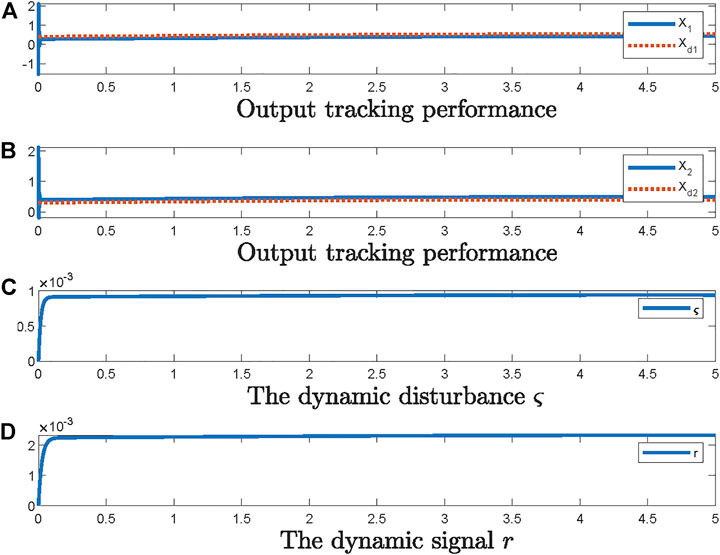
FIGURE 1. Output tracking performance and evolution of dynamic uncertainties.

6 Conclusion

In this study, a control approach for MIMO strict feedback nonlinear unmodeled dynamical systems with CFs is developed. The dynamic signal design introduced together with RBFNNs can efficiently prevent the effect of the dynamic uncertainties. The CFs employed in the controller design can not only prevent the explosion of complexity, but can also eliminate the effect of filter errors through the compensating signal design. Compared with single-input single-output strict feedback nonlinear systems, the approach proposed in this study is suitable for more general cases. Finally, in the simulation experiments, the presented method is applied to power systems, where the simulation results validate the effect of the scheme proposed.

Data Availability Statement

The original contributions presented in the study are included in the article/Supplementary Material, further inquiries can be directed to the corresponding author.

Author Contributions

XF, LS, and YZ contributed to conception and design of this study. XF investigated the theoretical analysis for the command filter design. LS performed the simulation study with application to an energy system. YZ organized the writing of the manuscript. XF, LS, and YZ collaborated to write all the sections of the manuscript. All authors contributed to manuscript revision, and read and approved the submitted version.

Funding

This work was supported by the Youth Innovation Promotion Association of Chinese Academy of Sciences under Grant 2020134.

Conflict of Interest

The authors declare that the research was conducted in the absence of any commercial or financial relationships that could be construed as a potential conflict of interest.

Publisher’s Note

All claims expressed in this article are solely those of the authors and do not necessarily represent those of their affiliated organizations, or those of the publisher, the editors, and the reviewers. Any product that may be evaluated in this article, or claim that may be made by its manufacturer, is not guaranteed or endorsed by the publisher.

References

Deese, J., and Vermillion, C. (2021). Recursive Gaussian Process-Based Adaptive Control, with Application to a lighter-Than-air Wind Energy System. IEEE Trans. Contr. Syst. Technol. 29, 1823–1830. doi:10.1109/TCST.2020.3014159

CrossRef Full Text | Google Scholar

Farrell, J. A., Polycarpou, M., Sharma, M., and Wenjie Dong, W. (2009). Command Filtered Backstepping. IEEE Trans. Automat. Contr. 54, 1391–1395. doi:10.1109/tac.2009.2015562

CrossRef Full Text | Google Scholar

Ghaffarzdeh, H., and Mehrizi-Sani, A. (2020). Mitigation of Subsynchronous Resonance Induced by a Type Iii Wind System. IEEE Trans. Sustain. Energ. 11, 1717–1727. doi:10.1109/TSTE.2019.2938014

CrossRef Full Text | Google Scholar

Ghosh, S., and Kamalasadan, S. (2017). An Integrated Dynamic Modeling and Adaptive Controller Approach for Flywheel Augmented Dfig Based Wind System. IEEE Trans. Power Syst. 32, 2161–2171. doi:10.1109/TPWRS.2016.2598566

CrossRef Full Text | Google Scholar

Han, Q., and Liu, X. (2020). Robust I&I Adaptive Control for a Class of Quadrotors with Disturbances. IEEE Access 8, 216519–216528. doi:10.1109/ACCESS.2020.3041030

CrossRef Full Text | Google Scholar

Hardy, G. H., Littlewood, J. E., and Pólya, G. (1952). Inequalities. Cambridge: Cambridge University Press.

Google Scholar

Hu, C., Ma, Y., Yu, J., and Zhao, L. (2020). Dynamic Surface Backstepping Control for Voltage Source Converter-High Voltage Direct Current Transmission Grid Side Converter Systems. Electronics 9, 9020333. doi:10.3390/electronics9020333

CrossRef Full Text | Google Scholar

Jiang, Z.-P., and Praly, L. (1998). Design of Robust Adaptive Controllers for Nonlinear Systems with Dynamic Uncertainties. Automatica 34, 825–840. doi:10.1016/s0005-1098(98)00018-1

CrossRef Full Text | Google Scholar

L'Afflitto, A. (2018). Barrier Lyapunov Functions and Constrained Model Reference Adaptive Control. IEEE Control. Syst. Lett. 2, 441–446. doi:10.1109/LCSYS.2018.2842148

CrossRef Full Text | Google Scholar

Li, C., Wu, Y., Sun, Y., Zhang, H., Liu, Y., Liu, Y., et al. (2020). Continuous Under-frequency Load Shedding Scheme for Power System Adaptive Frequency Control. IEEE Trans. Power Syst. 35, 950–961. doi:10.1109/TPWRS.2019.2943150

CrossRef Full Text | Google Scholar

Liu, L., Liu, Y.-J., Tong, S., and Gao, Z. (2022). Relative Threshold-Based Event-Triggered Control for Nonlinear Constrained Systems with Application to Aircraft wing Rock Motion. IEEE Trans. Ind. Inf. 18, 911–921. doi:10.1109/TII.2021.3080841

CrossRef Full Text | Google Scholar

Liu, L., Zhao, W., Liu, Y.-J., Tong, S., and Wang, Y.-Y. (2021). Adaptive Finite-Time Neural Network Control of Nonlinear Systems with Multiple Objective Constraints and Application to Electromechanical System. IEEE Trans. Neural Netw. Learn. Syst. 32, 5416–5426. doi:10.1109/TNNLS.2020.3027689

PubMed Abstract | CrossRef Full Text | Google Scholar

Mukherjee, S., Chowdhury, V. R., Shamsi, P., and Ferdowsi, M. (2017). Model Reference Adaptive Control Based Estimation of Equivalent Resistance and Reactance in Grid-Connected Inverters. IEEE Trans. Energ. Convers. 32, 1407–1417. doi:10.1109/TEC.2017.2710200

CrossRef Full Text | Google Scholar

Namazi, M. M., Nejad, S. M. S., Tabesh, A., Rashidi, A., and Liserre, M. (2018). Passivity-based Control of Switched Reluctance-Based Wind System Supplying Constant Power Load. IEEE Trans. Ind. Electron. 65, 9550–9560. doi:10.1109/TIE.2018.2816008

CrossRef Full Text | Google Scholar

Nascimento Moutinho, M., da Costa, C. T., Barra, W., and Augusto Lima Barreiros, J. (2008). Self-tunning Control Methodologies Applied to the Automatic Voltage Control of a Synchronous Generator. IEEE Latin Am. Trans. 6, 408–418. doi:10.1109/TLA.2008.4839110

CrossRef Full Text | Google Scholar

Quan, X., Yu, R., Zhao, X., Lei, Y., Chen, T., Li, C., et al. (2020). Photovoltaic Synchronous Generator: Architecture and Control Strategy for a Grid-Forming Pv Energy System. IEEE J. Emerg. Sel. Top. Power Electron. 8, 936–948. doi:10.1109/JESTPE.2019.2953178

CrossRef Full Text | Google Scholar

Wang, D., and Huang, J. (2005). Neural Network-Based Adaptive Dynamic Surface Control for a Class of Uncertain Nonlinear Systems in Strict-Feedback Form. IEEE Trans. Neural Netw. 16, 195–202. doi:10.1109/tnn.2004.839354

PubMed Abstract | CrossRef Full Text | Google Scholar

Wang, L., Li, H., Zhou, Q., and Lu, R. (2017). Adaptive Fuzzy Control for Nonstrict Feedback Systems with Unmodeled Dynamics and Fuzzy Dead Zone via Output Feedback. IEEE Trans. Cybern. 47, 2400–2412. doi:10.1109/TCYB.2017.2684131

PubMed Abstract | CrossRef Full Text | Google Scholar

Wang, Y., Cao, L., Zhang, S., Hu, X., and Yu, F. (2016). Command Filtered Adaptive Fuzzy Backstepping Control Method of Uncertain Non‐linear Systems. IET Control. Theor. & amp; Appl. 10, 1134–1141. doi:10.1049/iet-cta.2015.0946

CrossRef Full Text | Google Scholar

Wu, C., Chen, J., Xu, C., and Liu, Z. (2017). Real-time Adaptive Control of a Fuel Cell/battery Hybrid Power System with Guaranteed Stability. IEEE Trans. Contr. Syst. Technol. 25, 1394–1405. doi:10.1109/TCST.2016.2611558

CrossRef Full Text | Google Scholar

Xia, X., and Zhang, T. (2018). Adaptive Quantized Output Feedback Dsc of Uncertain Systems with Output Constraints and Unmodeled Dynamics Based on Reduced-Order K-Filters. Neurocomputing 310, 236–245. doi:10.1016/j.neucom.2018.05.031

CrossRef Full Text | Google Scholar

Xu, D., Liu, J., Yan, X.-G., and Yan, W. (2018). A Novel Adaptive Neural Network Constrained Control for a Multi-Area Interconnected Power System with Hybrid Energy Storage. IEEE Trans. Ind. Electron. 65, 6625–6634. doi:10.1109/TIE.2017.2767544

CrossRef Full Text | Google Scholar

Yang, Y., Gao, W., Modares, H., and Xu, C.-Z. (2021a). Robust Actor-Critic Learning for Continuous-Time Nonlinear Systems with Unmodeled Dynamics. IEEE Trans. Fuzzy Syst. 2021, 1. doi:10.1109/TFUZZ.2021.3075501

CrossRef Full Text | Google Scholar

Yang, Y., Kiumarsi, B., Modares, H., and Xu, C. (2021b). Model-Free λ-Policy Iteration for Discrete-Time Linear Quadratic Regulation. IEEE Trans. Neural Netw. Learn. Syst. 2021, 1–15. doi:10.1109/TNNLS.2021.3098985

CrossRef Full Text | Google Scholar

Yang, Y., Liu, Z., Li, Q., and Wunsch, D. C. (2021c). Output Constrained Adaptive Controller Design for Nonlinear Saturation Systems. Ieee/caa J. Autom. Sinica 8, 441–454. doi:10.1109/JAS.2020.1003524

CrossRef Full Text | Google Scholar

Yang, Y., Modares, H., Vamvoudakis, K. G., He, W., Xu, C.-Z., and Wunsch, D. C. (2021d). Hamiltonian-driven Adaptive Dynamic Programming with Approximation Errors. IEEE Trans. Cybern. 2021, 1–12. doi:10.1109/TCYB.2021.3108034

CrossRef Full Text | Google Scholar

Yang, Y., Vamvoudakis, K. G., Modares, H., Yin, Y., and Wunsch, D. C. (2021e). Hamiltonian-driven Hybrid Adaptive Dynamic Programming. IEEE Trans. Syst. Man. Cybern, Syst. 51, 6423–6434. doi:10.1109/TSMC.2019.2962103

CrossRef Full Text | Google Scholar

Yang, Y., Vamvoudakis, K. G., Modares, H., Yin, Y., and Wunsch, D. C. (2020). Safe Intermittent Reinforcement Learning with Static and Dynamic Event Generators. IEEE Trans. Neural Netw. Learn. Syst. 31, 5441–5455. doi:10.1109/TNNLS.2020.2967871

PubMed Abstract | CrossRef Full Text | Google Scholar

Zhao, J., Tong, S., and Li, Y. (2021a). Fuzzy Adaptive Output Feedback Control for Uncertain Nonlinear Systems with Unknown Control Gain Functions and Unmodeled Dynamics. Inf. Sci. 558, 140–156. doi:10.1016/j.ins.2020.12.092

CrossRef Full Text | Google Scholar

Zhao, L., Yu, J., and Wang, Q.-G. (2021b). Finite-time Tracking Control for Nonlinear Systems via Adaptive Neural Output Feedback and Command Filtered Backstepping. IEEE Trans. Neural Netw. Learn. Syst. 32, 1474–1485. doi:10.1109/tnnls.2020.2984773

PubMed Abstract | CrossRef Full Text | Google Scholar

Zhu, G., Du, J., and Kao, Y. (2018). Command Filtered Robust Adaptive Nn Control for a Class of Uncertain Strict-Feedback Nonlinear Systems under Input Saturation. J. Franklin Inst. 355, 7548–7569. doi:10.1016/j.jfranklin.2018.07.033

CrossRef Full Text | Google Scholar

Zou, W., Shi, P., Xiang, Z., and Shi, Y. (2020a). Consensus Tracking Control of Switched Stochastic Nonlinear Multiagent Systems via Event-Triggered Strategy. IEEE Trans. Neural Netw. Learn. Syst. 31, 1036–1045. doi:10.1109/tnnls.2019.2917137

PubMed Abstract | CrossRef Full Text | Google Scholar

Zou, W., Shi, P., Xiang, Z., and Shi, Y. (2020b). Finite-time Consensus of Second-Order Switched Nonlinear Multi-Agent Systems. IEEE Trans. Neural Netw. Learn. Syst. 31, 1757–1762. doi:10.1109/tnnls.2019.2920880

PubMed Abstract | CrossRef Full Text | Google Scholar