Interval Prediction of Building Foundation Settlement Using Kernel Extreme Learning Machine

Dynamic building foundation settlement subsidence threatens urban businesses and residential communities. In the temporal domain, building foundation settlement is often dynamic and requires real-time monitoring. Accurate quantification of the uncertainty of foundation settlement in the near future is essential to advanced risk management for buildings. Traditional models for predicting foundation settlement mostly utilize the point estimates approach, which provides a single value that can be close or distant from the actual one. However, such an estimation fails to quantify estimation uncertainties. The interval prediction, as an alternative, can provide a prediction interval for the ground settlement with high confidence bands. This study, proposes a lower upper bound estimation approach integrated with a kernel extreme learning machine to predict ground settlement levels with prediction intervals in the temporal domain. A revised objective function is proposed to further improve the interval prediction performance. In this study, the proposed method is compared to the artificial neural network and classical extreme learning machine. Building settlement data collected from Fuxing City, Liaoning Province in China was used to validate the proposed approach. The comparative results show that the proposed approach can construct superior prediction intervals for foundation settlement.

Introduction

Ground settlement is a common geological phenomenon and poses a risk to local communities. The major factor that induces ground settlement is soil liquefaction, which softens soil and causes buildings to settle more than the soil (Feng et al., 2021; Li et al., 2022). Consequently, the shear stresses and contact pressure imposed by buildings change due to soil softening and impact building settlement levels (Karimi et al., 2018; Wei et al., 2020). Settlement is an incremental process and is dynamic in the temporal domain; therefore, settlement prediction is important for managing the potential risk of structural damage in buildings (Feng et al., 2018; Dong et al., 2019). Hence, it is necessary to predict foundation settlement in the temporal domain.

In the literature review, soil physics, and numerical simulations have been widely discussed for modeling ground settlement. Dashti et al. (2010) investigated the mechanism of building foundation settlement and discovered that it is greatly dependent on the characteristics of earthquake motion, liquefiable soil, and buildings. Bullock et al. (2019) developed a physics-based semi-empirical probabilistic model to assess the risk of liquefaction-induced permanent building settlement using 50 case studies. According to Peduto et al. (2013), synthetic aperture radar sensors used in advanced differential interferometric techniques (generically called “DInSAR”), are widely applied to compute settlement severity. The “DInSAR” denotes a remote sensing technique that allows us to analyze deformation phenomena by exploiting the phase difference (usually referred to as interferogram) of SAR image pairs relevant to an area under study. It allows the generation of mean deformation velocity maps and displacement time series from a data set of subsequently acquired SAR images (Gabriel et al., 1989). Ng et al. (2015) performed a series of 3D centrifuge model tests to investigate the ground settlement caused by piggyback twin tunneling. Wang et al. (2019) conducted shake-table tests to analyze the relationship between foundation settlement and the degree of soil liquefaction. Zhang et al. (2020) constructed a 3D fluid-solid coupling finite element model to simulate the ground responses induced by tunneling crossing the interface of water-bearing mixed ground. Such approaches can be successfully applied to case-specific geological conditions. However, ground subsidence is a complex system with heterogeneous geological and geomechanical characteristics. Hence, a more comprehensive approach is needed to model and predict ground settlement that can be applied to a variety of cases with heterogeneous conditions.

Machine learning algorithms have demonstrated their effectiveness and accuracy in modeling ground settlement (Li et al., 2021b). Santos and Celestino (2008) utilized artificial neural networks (ANNs) to predict tunnel-induced settlement in the case study of the Säo Paulo subway construction. Gong et al. (2014) conducted a site exploration and Monte Carlo simulation to study tunnel-induced settlement in clays. Wei and Yang (2018) predicted coal-mining induced ground settlement using an online sequential extreme learning machine. Moosazadeh et al. (2019) integrated the particle swarm optimization algorithm and optimized an artificial neural network to predict the structural damage of buildings caused by foundation settlement. Liu et al. (2020) utilized data mining to select important predictor variables and predict the foundation settlement grout holes in a building basement. Recent research has demonstrated that machine learning algorithms have the potential to become a comprehensive and reliable approach for studying building foundation settlement. Nevertheless, all machine learning approaches utilize a point-estimation approach that does not sufficiently address the uncertainties in the settlement process, which is largely dynamic. An interval-based prediction approach is a feasible solution to address this deficiency.

Among popular machine learning algorithms, the extreme learning machine (ELM) (Huang et al., 2006) has attracted significant attention in the machine learning community in recent years (He et al., 2017a; Xu et al., 2019; Li et al., 2020; Ouyang et al., 2020; Li et al., 2021a; Li 2022a). The ELM algorithm is a single hidden-layer feedforward network that produces promising predictive modeling results across various domains in engineering. For example, Li et al. (2018) integrated Least Absolute Shrinkage and Selection Operator -ELM with parametric copula models to model and forecast geological landslide displacement in the temporal domain. He and Kusiak. (2018) utilized a linear ensemble of multiple ELMs to forecast wind turbine power generation in the renewable energy sector. Ouyang et al. (2018) developed a data-driven framework to automatically classify mechanical error codes within wind turbines. Wei and Yang (2018) first proposed using an online sequential ELM to predict coal-mining induced ground subsidence. The Cox proportional hazard regression model was used to screen the numerical and categorical geological features and the OS-ELM was used to predict the maximum subsidence by inputting the selected features. The above research demonstrates that ELMs outperforms both regression and classification tasks.

Based on the above discussion, this study proposed, a data-driven approach using a kernel extreme learning machine (KELM) integrated with lower-upper bound estimation. First, an interval prediction framework was utilized in the building foundation settlement study and a lower upper bound estimation (LUBE) method was adopted. Second, a KELM was introduced in this study and the selection of the kernels was optimized using a cross-validation experiment. A comparative analysis was performed against state-of-the-art approaches, such as ANNs and classical ELMs. The computational results demonstrated that the proposed approach is feasible and outperforms other methods used for studying building foundation settlement.

The main contribution of this paper is as follows:

• First, it proposed an interval prediction framework to estimate future foundation settlement with quantified uncertainties. A LUBE method was applied in the study.

• Second, it utilized a KELM to enhance the predictive performance of future foundation settlement. A comparative analysis across multiple kernels was conducted to select the optimal kernel for the case studies.

To realize this proposed approach, this paper is organized as follows. Section 2 introduces the data collection process and mathematically defines the underlying problem. Section 3 provides a detailed description of the methods used in this study. Section 4 compares the performance of the models on the geological data collected from the monitoring sites. Finally, Section 5 concludes the study.

Foundation Settlement and Problem Formulation

Foundation Settlement

In northern China, building foundation settlement is a common event and has resulted in millions of dollars of economic losses and several casualties. The major cause of foundation settlement can be attributed to soil liquefaction, which changes the shear stress in the foundation soil (Dong et al., 2020; Fan et al., 2022). This results in deviatoric deformation within the liquefiable soil beneath the building foundation and volumetric strains due to localized drainage during shaking (Lu et al., 2019). Consequently, the building foundation will be unevenly settled and potentially have dynamic structural movement as illustrated in Figure 1.

FIGURE 1

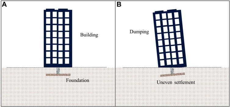
FIGURE 1. Schematic diagram of building foundation settlement.

In engineering geology societies, engineers would construct physics models to compute and forecast foundation settlement, depending on the effect of gravity on the building (Cui et al., 2021; Zhou et al., 2021). However, in practice, there is always a difference between the theoretical settlement and actual settlement curves. As illustrated in Figure 2, actual settlement monitoring and forecasting is a post-hoc analysis that can benefit the risk management process of the building structure.

FIGURE 2

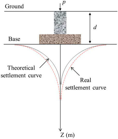
FIGURE 2. Vertical diagram of the theoretical and actual settlement.

Our case study area is in Fuxin City, Liaoning Province, China where many buildings are between 20 and 30 years old, are located in urbanized areas or suburbs, and experience uneven foundation settlement. Natural changes in groundwater levels are exacerbated by anthropogenic activities which have caused and accelerated soil liquefaction, resulting in foundation settlement (Fan and Cai 2021). In recent years, several meter-long cracks have emerged in building foundations and at the lower level of walls. The location of our study area and photographs of building foundation settlement are shown in Figure 3.

FIGURE 3

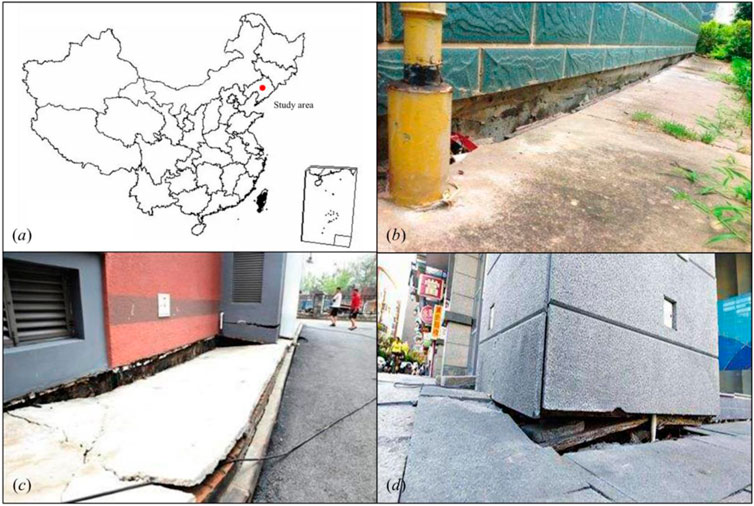
FIGURE 3. Case study area and settlement examples.

Data Collection

The dataset was collected by experts from Liaoning Technical University, School of Geomatics and their working institution is near our case study area. They have spent several years monitoring the settlement of multiple buildings in town and local suburb area.

A diagram illustrating the time-series of settlement is shown in Figure 4. In the four building case studies, a monitoring point was configured at the edge of the building. The location was set to 4 m above the ground level as the initial setting. Altitude was measured from the ground level daily, using the absolute difference from the previous day’s measurement as the incremental settlement change. For each case study, two to three monitoring points were used to avoid measurement errors from a single point.

FIGURE 4

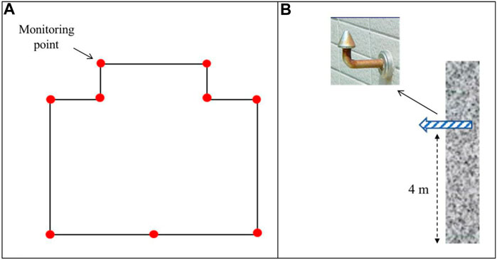
FIGURE 4. Data collection process of foundation settlement.

The dataset contains the daily monitored foundation settlement from January 2013 to April 2013. We selected the point with the largest cumulative settlement for each case study. In total, 120 time-series observations were obtained for each building. The basic information of the dataset is provided in Table 1, which includes the unit, building type, maximum daily settlement, maximum cumulative settlement, mean daily settlement, and standard deviation of the daily settlement.

TABLE 1

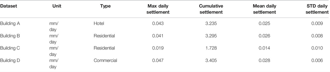
TABLE 1. Description of the foundation settlement dataset of the four case study buildings.

Problem Formulation

The main objective of this research is to develop a data-driven framework to predict the interval of possible foundation settlement values in the temporal domain. For each case study, the foundation settlement was monitored daily and the target was to predict the incoming daily settlement value. The underlying problem is formulated in Eq. 1:

$x_t=f(x_{t-1},x_{t-2},\dots ,x_{t-k})(1)$

Where $x_t$ represents the instant settlement in the future at time t and $x_{t-k}$ denotes the historic lagged settlement based on the actual measurement. To predict the settlement for a period, this study adopted the sequential prediction strategy introduced in Section 3.5.

Materials and Methods

Auto-Correlation Analysis

The daily foundation settlement is a time-series data format in the temporal domain. In many cases, the daily settlement always reflects strong statistical patterns including seasonality and autocorrelation (Zhou et al., 2018). The identification of such patterns is essential to the construction of time-series prediction models as it determines the optimal input size. Here, two fundamental statistical indices are adopted to discover the statistical autocorrelation patterns: the autocorrelation function (ACF) and the partial autocorrelation function (PACF).

The ACF measures Pearson’s correlation coefficient between the current settlement and its k-lagged historic settlement series. Meanwhile, the PACF computes the additional contribution from the lag-k series to the current settlement, which is nonzero in most cases. The ACF and PACF are computed using Eqs. 2, 3 (Ouyang et al., 2017):

${\rho }_k=\frac{Cov(x_t,x_{t-k})}{\sqrt{Var\left(x_t\right)Var\left(x_{t-k}\right)}}(2)$

${\varnothing }_k=corr\left(x_t,x_{t-k}\text{|}{x}_t,x_{t-1},\dots ,x_{t-k-1}\right)(3)$

where $x_t$ and $x_{t-k}$ are the current and k-lagged settlement series, respectively, ${\rho }_k$ is the ACF, and ${\varnothing }_k$ is the PACF, which computes the conditional correlation between $x_t$ and $x_{t-k}$.

Kernel Extreme Learning Machine

An ELM (Huang et al., 2006) is a single hidden-layer feedforward neural network. Compared with classical artificial neural networks, it contains only three components: an input layer, a single hidden layer, and an output layer. Given a pair of input/output data samples ($x_i,y_i$), the classical ELM can be formulated in Eq. 4 (Wei and Yang 2018):

${\displaystyle \sum }_{i=1}^N{\beta }_{i}h\left(x_i\right)=y_i(4)$

Where $\beta$_i represents the weight vector that connects the jth hidden neuron to the output neuron. The $h\left(x_i\right)$ serves as a general mapping function that maps the input features into latent space (He and Kusiak. 2018). Hence, a compact form of an ELM can be written as Eq. 5:

$\mathit{H}\mathit{\beta }=\mathit{y}(5)$

Where $\mathit{H}$ and $\mathit{\beta }$ are expressed as follows:

$\mathit{H}=\left[\begin{array}{ccc}{h}_1\left({\mathrm{x}}_{\mathrm{1}}\right)& \cdots & h_L\left({\mathrm{x}}_{\mathrm{1}}\right)\\ ⋮& \ddots & ⋮\\ h_1\left({\mathrm{x}}_{\mathrm{N}}\right)& \cdots & h_L\left({\mathrm{x}}_{\mathrm{N}}\right)\end{array}\right](6)$

$\mathit{\beta }=[{\mathit{\beta }}_1,{\mathit{\beta }}_2,\dots ,{\mathit{\beta }}_N](7)$

To obtain the optimal solution for the ELM, the least-squares solution can be computed using Eq. 8 as follows:

$\tilde{\mathit{\beta }}={\mathit{H}}^{†}\mathit{y}(8)$

Where † denotes the Moore-Penrose generalized inverse. Figure 5A depicts the classical structure of the ELM algorithm.

FIGURE 5

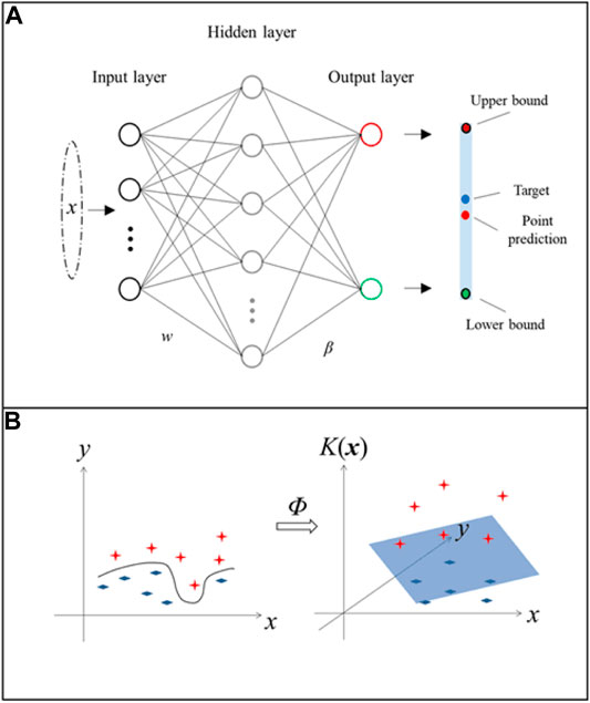
FIGURE 5. Schematic diagram of kernel extreme learning machine.

In addition to the classical ELM, owing to unknown/unspecified feature mapping, we cannot calculate the Moore-Penrose inverse in Eq. 8. Hence, a kernel version of ELM can be obtained by defining the kernel matrix as follows:

$\mathit{K}= \mathit{H}{\mathit{H}}^T (9)$

${\mathit{K}}_{\mathit{i}\mathit{j}}=h\left({\mathbf{x}}_{\mathit{i}}\right)h{\left({\mathbf{x}}_{\mathit{j}}\right)}^T= k({\mathrm{x}}_{\mathit{i}},{\mathrm{x}}_{\mathit{j}})(10)$

Where $K$ is the kernel matrix. The output function of KELM for a new testing observation can be computed using Eq. 11 as follows:

$S= h\left(\widehat{\mathit{x}}\right)\tilde{\mathit{\beta }}= h\left(\widehat{\mathrm{x}}\right){\mathit{H}}^T{\left(\mathit{H}{\mathit{H}}^T\right)}^{-1}y={\left[\begin{array}{c}k(\tilde{\mathrm{x}},{\mathrm{x}}_{\mathrm{1}})\\ ⋮\\ k(\tilde{\mathrm{x}},{\mathrm{x}}_{\mathrm{N}})\end{array}\right]}^T{\mathit{K}}^{†}\mathbf{y}(11)$

In this study, we examined the effectiveness of two popular kernels, the Gaussian kernel Eq. 12 and polynomial kernel Eq. 13, which are expressed as:

$k_1\left({\mathbf{x}}_{\mathrm{i}},{\mathbf{x}}_{\mathrm{j}}\right)=\exp \left(-\frac{||{\mathbf{x}}_{\mathrm{i}}-{\mathbf{x}}_{\mathrm{j}}||}{2{\sigma }^2}\right)(12)$

$k_2\left({\mathbf{x}}_{\mathrm{i}},{\mathbf{x}}_{\mathrm{j}}\right)={\left({\mathbf{x}}_{\mathrm{i}}^T{\mathbf{x}}_{\mathrm{j}}\right)}^d(13)$

Where $\sigma$ is the kernel width and d denote the polynomial degree. An explicit interpretation of the effect of the kernel function is presented in Figure 5B.

Prediction Interval Formulation Using the Lower Upper Bound Estimation Method

Prediction intervals (PIs) are widely used to quantify the uncertainty in prediction models (Li 2022b). Given an input feature vector x_i, a PI with a confidence level of 100% (1-α) constructed for the prediction target y_i, can be expressed in (14) as follows:

${\widehat{I}}^{\left(\alpha \right)}\left(x_i\right)=[{\widehat{L}}^{\left(\alpha \right)}\left(x_i\right),{\widehat{U}}^{\left(\alpha \right)}\left(x_i\right)](14)$

Where α denotes the quantile of the standard normal distribution and ${\widehat{L}}^{\left(\alpha \right)}\left(x_i\right)$ and ${\widehat{U}}^{\left(\alpha \right)}\left(x_i\right)$ are the lower and upper bounds of the ith PI, respectively, as illustrated in Figure 5A. The predicted target settlement is expected to be covered by ${\widehat{I}}^{\left(\alpha \right)}\left(x_i\right)$ with a coverage probability expressed by Eq. 15:

$P({\widehat{L}}^{\left(\alpha \right)}\left(x_i\right)\le y_i\le {\widehat{U}}^{\left(\alpha \right)}\left(x_i\right)=100\left(1-\alpha \right)\%(15)$

In this study, the LUBE method was adopted to customize the KELM model as presented in Section 3.2. PIs were constructed as outputs for the KELM algorithm. As shown in Figure 5 the proposed KELM contains two output neurons. The upper and lower bounds can be formulated in Eqs. 16, 17 as follows:

${\widehat{U}}^{\left(\alpha \right)}\left(x_i\right)=\text{max}\{o_{j1},o_{j2}\}(16)$

${\widehat{L}}^{\left(\alpha \right)}\left(x_i\right)=\text{min}\{o_{j1},o_{j2}\}(17)$

Where x_j denotes the jth input and $o_{j1}$ and $o_{j2}$ are the lower and upper outputs for the jth input sample, respectively, as shown in Figure 6.

FIGURE 6

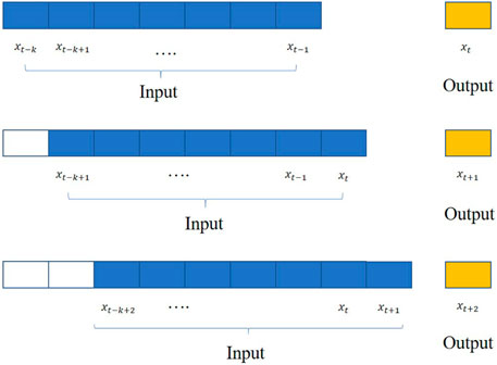
FIGURE 6. Sequential prediction strategy.

Training and Testing Strategies

In this study, the historic lagged settlement values were selected as inputs and the future settlement value as the output. We collected 120 settlement observations from January 2013 to April 2013 from each case study. Ninety observations between January and March 2013 were used as the training/validation set and the remaining 30 observations in April 2013 were used as the testing dataset.

To predict the settlement, a sequential prediction strategy was adopted to predict the periodic foundation settlement, as shown in Figure 6.

As shown in Figure 6, the inputs and outputs are defined in the time-series prediction model. The k historic values of the settlements were used as inputs in the prediction model. The optimal value of k is determined by the autocorrelation analysis considering the computed ACFs and PACFs. A single settlement at time t is the output of the prediction model. To predict the settlement at time t+1, the predicted settlement at time t and its k-lagged historic settlement values were selected as the new inputs. The output was the settlement at time t+1. After training it repeatedly in a sequential manner, the periodic incoming settlement was predicted and compared with ground truth data for model evaluation.

Evaluation Metric and Loss Function

In this study, two widely used metrics, namely prediction interval coverage probability (PICP) and prediction interval normalized average width (PINAW) (Ouyang et al., 2019) were used to measure the performance of prediction intervals. The PICP and PINAW can be computed using Eqs 18, 19:

$PICP=\frac{{{\displaystyle \sum }}_{i=1}^N{c}_i}{N}(18)$

$PINAW=\frac{{{\displaystyle \sum }}_{i=1}^N[{\widehat{L}}^{\left(\alpha \right)}\left(x_i\right),{\widehat{U}}^{\left(\alpha \right)}\left(x_i\right)]}{y_{max}-y_{min}}(19)$

Where $N$ represents the number of observations and $y_{max}$ and $y_{min}$ are the minimum and maximum values of the true target, respectively. Variable $c_i$ is a binary indicator function that determines whether the target falls into the limit of PI which can be expressed in Eq. 20 as follows:

$c_i=\{\begin{array}{c}\begin{array}{cc}1& y_i\in [{\widehat{L}}^{\left(\alpha \right)}\left(x_i\right),{\widehat{U}}^{\left(\alpha \right)}\left(x_i\right)]\end{array}\\ \begin{array}{cc}0& y_i\notin [{\widehat{L}}^{\left(\alpha \right)}\left(x_i\right),{\widehat{U}}^{\left(\alpha \right)}\left(x_i\right)]\end{array}\end{array}(20)$

In general, the PICP evaluates the probability that the prediction target falls within the bound between the upper and lower limits. The value of PICP ranges between 0 and 1. The PINAW denotes the mean width of the PIs. In most cases, high PICP values and low PINAW values indicate high-quality PIs (Sun et al., 2017).

The PICP and PINAW are two conflicting properties. To maintain a comprehensive balance between the two metrics, a cost function, namely the coverage width-based criterion (CWC), was used in this study. The CWC can be computed using Eq. 21.

$CWC=PINAW(1+\gamma \left(PICP\right)e^{-\eta (PICP-\mu )})(21)$

Where the parameters $\eta$ and $\mu$ are used to define the penalty term $e^{-\eta (PICP-\mu )}$ to maintain the balance between $PINAW$ and $PICP$ and $\gamma \left(\right)$ is used to reduce the risk of the PI constraint violation during the training process. When predicting building foundation settlement, it is difficult to adjust the optimal balance between the coverage of the forecast interval and the interval width under different settlement speeds through $\eta$. Thus, a revised version of the CWC is proposed in this study to increase the power of the penalty parameter, as expressed in Eq. 22:

$CW{C}_{proposed}=(\mathit{\alpha }+\mathit{\beta \; \ast }PINAW)(1+\gamma \left(PICP\right)e^{-\eta (PICP-\mu )})(22)$

Where parameter $\mathit{\beta }$ linearly amplifies the $PINAW$ and parameter $\mathit{\alpha }$ is used to avoid disappearance if $CW{C}_{proposed}$ is too small. In this research, the $CW{C}_{proposed}$ is used as the objective function to train the KELM following the LUBE approach.

Benchmarking Methods

In this research, the ANN and classical ELM were selected as benchmarking algorithms for the comparative analysis. The classical ELM is described in detail in Section 3.2, where the only difference compared with the KELM is the kernel function utilized for feature mapping.

The ANN is a non-parametric algorithm developed based on cognitive learning processes and is capable of accurately predicting patterns that are not part of the training dataset. The structure of the ANN algorithm permits accurate mapping between the input and output in a highly nonlinear system (He et al., 2017b).

The neuron is the most essential element that functions within an ANN. With multiple neurons stacked in the hidden layers, nonlinear mapping between the input features and output can be expressed as Eq. 23:

$y=\phi ({\displaystyle \sum }_{i=1}^n{w}_i{x}_i+b)(23)$

Where x_j represents the jth input feature, w_j is the weight associated with the jth input, b is the bias, and $\phi$ is the activation function. In this study, the ANN was also customized using the LUBE method and the sigmoid activation function.

Results

Auto-Correlation Analysis

The selection of the optimal input feature set affect the performance of the data-driven models. Inspired by the ARIMA model, the ACF and PACF are computed between the current settlement and its k-lagged historic settlement to investigate the autocorrelation and seasonality within the dataset. The combination of the ACF and PACF results determines the final input feature sets.

As illustrated in Figure 7, the ACFs and PACFs were computed for the four time-series datasets for the four case study buildings listed in Table 1. The Ljung-Box test statistic was used to measure the statistical significance of the correlation coefficients. As shown in Figure 7, the blue lines serve as the threshold of the Ljung-Box test statistic and any lagged series with coefficients outside the band region are considered significant and thus, statistically impact the current settlement.

FIGURE 7

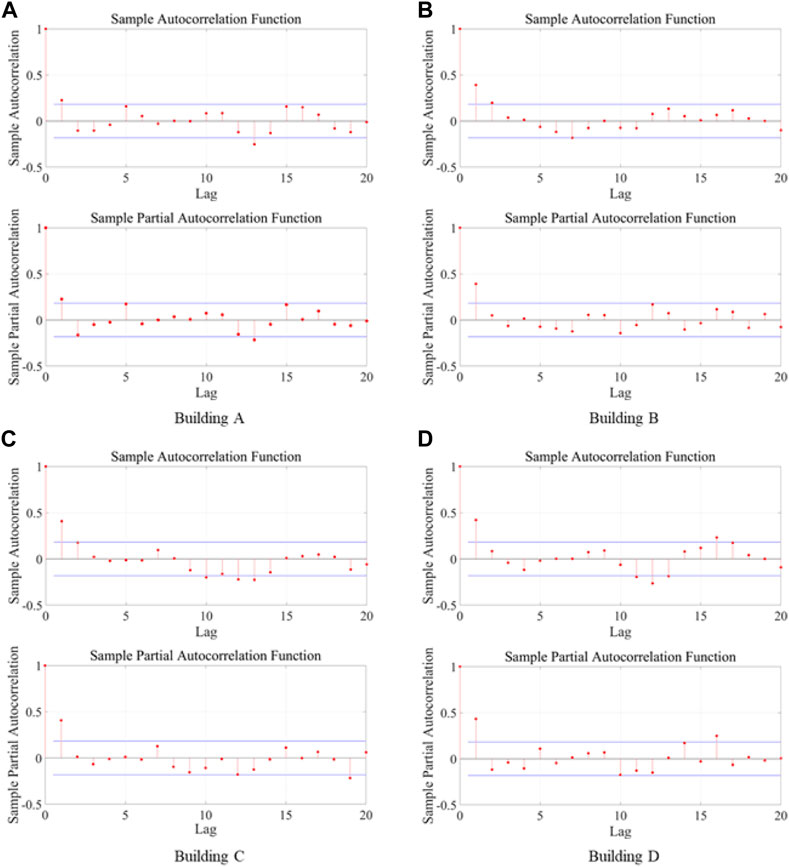
FIGURE 7. Computed ACFs and PACFs for the four cases study time-series.

Based on the computational results of the ACFs and PACFs, the optimal number of lagged series that can be selected as inputs for the time-series model for building A’s settlement data is 13. For buildings B and C, the optimal numbers of lagged series are 7 and 19, respectively. In addition, the number of lagged series selected as inputs was 16 for building D.

Hyper-Parameter Optimization

After the selection of the optimal input series, three algorithms, including the ANN, classical ELM, and KELM were selected for training and validating the time-series prediction model. Tuning the hyperparameters is an essential component of the process to ensure that the models can achieve optimal prediction performance.

Table 2 lists the number of hyperparameters for the three algorithms and the various initial settings of the parameters. For the ANN algorithm, two hyperparameters required optimization: the number of hidden layers and the number of hidden neurons in each layer. In the classical ELM algorithm, the number of hidden neurons within the hidden layer was the only hyperparameter that required optimization. The hyperparameters of the KELM included the number of hidden neurons in the hidden layer and the selection of kernel functions for feature mapping. The PICP was selected as the measurement metric for the selection of optimal hyperparameter settings for the three algorithms listed above.

TABLE 2

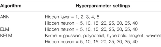
TABLE 2. List of hyperparameters tested for ANN, ELM, and KELM.

According to the computational results, the ANN algorithm with two hidden layers and 10 hidden neurons in each layer, had the smallest PICP value. For the classical ELM, the optimal number of hidden neurons was 15. For the KELM algorithm, the best performing kernel function was the Gaussian kernel and the optimal number of hidden neurons was 15. The training of the optimal setting of the KELM for the building settlement time-series data of all four cases is presented in Figures 8, 9.

FIGURE 8

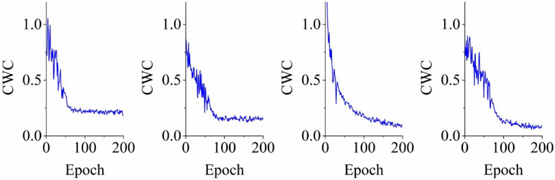
FIGURE 8. Training KELM on the four case study buildings using original CWC.

FIGURE 9

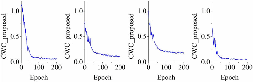
FIGURE 9. Training KELM on the four case study buildings using proposed CWC.

As shown in Figure 8, the original CWC decreased as the number of training epochs increased. For the four case studies, convergence of the original CWC occurred between 50 and 100 epochs. In comparison, as illustrated in Figure 9, the proposed CWC converged faster with a sharper gradient. This phenomenon can be attributed to parameter $\mathit{\beta }$ linearly amplifying the $PINAW$ and thus accelerating the convergence process. For all four buildings, the convergence of the proposed CWC occurred around the 50th epoch, which was comparatively faster than the original CWC, displayed in Figure 8. The experimental results confirm the superiority of the proposed CWC over the original CWC in training the KELM using the LUBE approach.

Foundation Settlement Prediction

Based on the obtained optimal settings for the hyperparameters, the prediction of the testing data for the four time-series settlements in April 2013 was performed. In this research, the prediction of the testing dataset was not evident, therefore, we adopted the sequential prediction strategy, as illustrated in Figure 6, to predict the daily incremental settlement of the four buildings. The prediction intervals were then overlaid with the actual measured incremental settlement as shown in Figure 10.

FIGURE 10

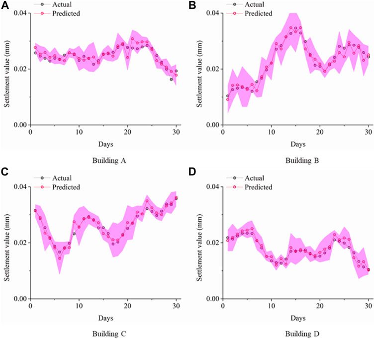
FIGURE 10. Prediction intervals constructed for the testing dataset using KELM.

As illustrated in Figure 10, prediction errors existed between the actual measured settlement and the predicted settlement. If we consider the systematic uncertainty in the prediction process, PIs can be constructed and the majority of the actual settlements fall within the 95% confidence level PIs according to the prediction outcome. However, since a few outliers fell outside the PIs, we used the overall measurement metrics (i.e., PICP and PINAW) to compute the overall prediction performance, as presented in Table 3.

TABLE 3

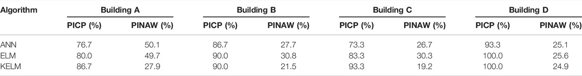
TABLE 3. PICP and PINAW of ANN, ELM, and KELM on the testing dataset.

As listed in Table 3, the PICP of the KELM integrated with the LUBE method was computed for the ANN, ELM, and KELM. In the settlement time-series of the four buildings, the KELM outperformed all the algorithms that were tested and produced the highest mean PICPs and lowest mean PINAWs. Based on the intrinsic formulation of these two metrics, the higher values of PICP and lower values of PINAW indicate more accurate and reliable interval prediction results. Hence, the effectiveness and robustness of the prediction power of the KELM with respect to interval prediction was demonstrated.

Conclusion

To predict building foundation settlement, a novel data-driven framework for interval prediction of time-series settlement prediction was presented in this study. First, the LUBE approach was applied to construct prediction intervals. Second, a kernel extreme learning machine was customized for the interval prediction task and predicted future settlement. Third, a revised version of the CWC was proposed to further improve the interval prediction performance. Four case studies in Liaoning Province were selected for this study and the daily settlement was monitored in the temporal domain. The computational results validated the superiority of the proposed algorithm by comparing it with benchmarking methods, including ANN and classical ELM.

The proposed approach is feasible to use this approach to monitor and assess building structural risks. The engineers can embed the proposed algorithm into the chip of the monitoring equipment and the predictions can be made in real-time. The settlement can be estimated in-advance and the risk analysis can be conducted by field engineers.

Data Availability Statement

The original contributions presented in the study are included in the article/supplementary material, further inquiries can be directed to the corresponding author.

Author Contributions

JD conceptualized the study, contributed to the study methodology, and wrote the original draft. TZ contributed to the study methodology, data curation and investigation and data analysis. JD and SY contributed to software and formal analysis. HF and WX contributed to investigation. All authors have read and agreed to the published version of the manuscript.

Funding

The study was supported by the Key Program of Science and Technology Planning Project of Deyang, China (Grant No.2018SZY108).

Conflict of Interest

The authors declare that the research was conducted in the absence of any commercial or financial relationships that could be construed as a potential conflict of interest.

Publisher’s Note

All claims expressed in this article are solely those of the authors and do not necessarily represent those of their affiliated organizations, or those of the publisher, the editors and the reviewers. Any product that may be evaluated in this article, or claim that may be made by its manufacturer, is not guaranteed or endorsed by the publisher.

Acknowledgments

We are also immensely grateful to the data collection from R. Sun from Sai Ding Engineering Co., Ltd. (formerly The Second Design Institute of the Ministry of Chemical Industry).

References

Bullock, Z., Karimi, Z., Dashti, S., Porter, K., Liel, A. B., and Franke, K. W. (2019). A Physics-Informed Semi-empirical Probabilistic Model for the Settlement of Shallow-Founded Structures on Liquefiable Ground. Géotechnique 69 (5), 406–419. doi:10.1680/jgeot.17.p.174

CrossRef Full Text | Google Scholar

Cui, S., Pei, X., Jiang, Y., Wang, G., Fan, X., Yang, Q., et al. (2021). Liquefaction within a Bedding Fault: Understanding the Initiation and Movement of the Daguangbao Landslide Triggered by the 2008 Wenchuan Earthquake (Ms = 8.0). Eng. Geol. 295, 106455. doi:10.1016/j.enggeo.2021.106455

CrossRef Full Text | Google Scholar

Dashti, S., Bray, J. D., Pestana, J. M., Riemer, M., and Wilson, D. (2010). Centrifuge Testing to Evaluate and Mitigate Liquefaction-Induced Building Settlement Mechanisms. J. Geotech. Geoenviron. Eng. 136 (7), 918–929. doi:10.1061/(asce)gt.1943-5606.0000306

CrossRef Full Text | Google Scholar

Dong, S., Feng, W., Yin, Y., Hu, R., Dai, H., and Zhang, G. (2020). Calculating the Permanent Displacement of a Rock Slope Based on the Shear Characteristics of a Structural Plane under Cyclic Loading. Rock Mech. Rock Eng. 53 (10), 4583–4598. doi:10.1007/s00603-020-02188-y

CrossRef Full Text | Google Scholar

Dong, S., Yi, X., and Feng, W. (2019). Quantitative Evaluation and Classification Method of the Cataclastic Texture Rock Mass Based on the Structural Plane Network Simulation. Rock Mech. Rock Eng. 52 (6), 1767–1780. doi:10.1007/s00603-018-1635-6

CrossRef Full Text | Google Scholar

Fan, Z., and Cai, J. (2021). Effects of Unidirectional In Situ Stress on Crack Propagation of a Jointed Rock Mass Subjected to Stress Wave. Shock Vib. 2021, 1. doi:10.1155/2021/5529540

CrossRef Full Text | Google Scholar

Fan, Z., Zhang, J., Xu, H., and Wang, X. (2022). Transmission and Application of a P-Wave across Joints Based on a Modified G-λ Model. Int. J. Rock Mech. Min. Sci. 150, 104991. doi:10.1016/j.ijrmms.2021.104991

CrossRef Full Text | Google Scholar

Feng, W., Dong, S., Wang, Q., Yi, X., Liu, Z., and Bai, H. (2018). Improving the Hoek-Brown Criterion Based on the Disturbance Factor and Geological Strength Index Quantification. Int. J. Rock Mech. Min. Sci. 108, 96–104. doi:10.1016/j.ijrmms.2018.06.004

CrossRef Full Text | Google Scholar

Feng, W., Lu, Z., Yi, X., and Dong, S. (2021). A Dynamic Method to Predict the Earthquake-Triggered Sliding Displacement of Slopes. Math. Problems Eng. 2021, 1. doi:10.1155/2021/4872987

CrossRef Full Text | Google Scholar

Gabriel, A. K., Goldstein, R. M., and Zebker, H. A. (1989). Mapping Small Elevation Changes over Large Areas: Differential Radar Interferometry. J. Geophys. Res. 94 (B7), 9183–9191. doi:10.1029/jb094ib07p09183

CrossRef Full Text | Google Scholar

Gong, C., Zeng, G., Ge, L., Tang, X., and Tan, C. (2014). Minimum Detectable Activity for NaI(Tl) Airborne γ-ray Spectrometry Based on Monte Carlo Simulation. Sci. China Technol. Sci. 57, 1840–1845. doi:10.1007/s11431-014-5553-x

CrossRef Full Text | Google Scholar

He, Y., Deng, J., and Li, H. (2017a). Short-term Power Load Forecasting with Deep Belief Network and Copula Models. 9th Int. Conf. intelligent human-machine Syst. Cybern. (IHMSC), 1, 191–194. doi:10.1109/ihmsc.2017.50

CrossRef Full Text | Google Scholar

He, Y., Kusiak, A., Ouyang, T., and Teng, W. (2017b). Data-driven Modeling of Truck Engine Exhaust Valve Failures: a Case Study. J. Mech. Sci. Technol. 31 (6), 2747–2757. doi:10.1007/s12206-017-0518-1

CrossRef Full Text | Google Scholar

He, Y., and Kusiak, A. (2018). Performance Assessment of Wind Turbines: Data-Derived Quantitative Metrics. IEEE Trans. Sustain. Energy 9 (1), 65–73. doi:10.1109/tste.2017.2715061

CrossRef Full Text | Google Scholar

Huang, G. B., Zhu, Q. Y., and Siew, C. K. (2006). Extreme Learning Machine: Theory and Applications. Neurocomputing 70 (1-3), 489–501. doi:10.1016/j.neucom.2005.12.126

CrossRef Full Text | Google Scholar

Karimi, Z., Dashti, S., Bullock, Z., Porter, K., and Liel, A. (2018). Key Predictors of Structure Settlement on Liquefiable Ground: a Numerical Parametric Study. Soil Dyn. Earthq. Eng. 113, 286–308. doi:10.1016/j.soildyn.2018.03.001

CrossRef Full Text | Google Scholar

Li, H., Deng, J., Feng, P., Pu, C., Arachchige, D. D. K., and Cheng, Q. (2021a). Short-Term Nacelle Orientation Forecasting Using Bilinear Transformation and ICEEMDAN Framework. Front. Energy Res. 9, 780928. doi:10.3389/fenrg.2021.780928

CrossRef Full Text | Google Scholar

Li, H., Deng, J., Yuan, S., Feng, P., and Arachchige, D. D. K. (2021b). Monitoring and Identifying Wind Turbine Generator Bearing Faults Using Deep Belief Network and EWMA Control Charts. Front. Energy Res. 9, 799039. doi:10.3389/fenrg.2021.799039

CrossRef Full Text | Google Scholar

Li, H., He, Y., Xu, Q., Deng, j., Li, W., and Wei, Y. (2022). Detection and Segmentation of Loess Landslides via Satellite Images: a Two-phase Framework. Landslides 19, 673–686. doi:10.1007/s10346-021-01789-0

CrossRef Full Text | Google Scholar

Li, H. (2022b). SCADA Data Based Wind Power Interval Prediction Using LUBE-Based Deep Residual Networks. Front. Energy Res. 10, 920837. doi:10.3389/fenrg.2022.920837

CrossRef Full Text | Google Scholar

Li, H. (2022a). Short-term Wind Power Prediction via Spatial Temporal Analysis and Deep Residual Networks. Front. Energy Res. 10, 920407. doi:10.3389/fenrg.2022.920407

CrossRef Full Text | Google Scholar

Li, H., Xu, Q., He, Y., and Deng, J. (2018). Prediction of Landslide Displacement with an Ensemble-Based Extreme Learning Machine and Copula Models. Landslides 15 (10), 2047–2059. doi:10.1007/s10346-018-1020-2

CrossRef Full Text | Google Scholar

Li, H., Xu, Q., He, Y., Fan, X., and Li, S. (2020). Modeling and Predicting Reservoir Landslide Displacement with Deep Belief Network and EWMA Control Charts: a Case Study in Three Gorges Reservoir. Landslides 17 (3), 693–707. doi:10.1007/s10346-019-01312-6

CrossRef Full Text | Google Scholar

Liu, Q., Xiao, F., and Zhao, Z. (2020). Grouting Knowledge Discovery Based on Data Mining. Tunn. Undergr. Space Technol. 95, 103093. doi:10.1016/j.tust.2019.103093

CrossRef Full Text | Google Scholar

Lu, Z., Yao, A., Su, A., Ren, X., Liu, Q., and Dong, S. (2019). Re-recognizing the Impact of Particle Shape on Physical and Mechanical Properties of Sandy Soils: a Numerical Study. Eng. Geol. 253, 36–46. doi:10.1016/j.enggeo.2019.03.011

CrossRef Full Text | Google Scholar

Moosazadeh, S., Namazi, E., Aghababaei, H., Marto, A., Mohamad, H., and Hajihassani, M. (2019). Prediction of Building Damage Induced by Tunnelling through an Optimized Artificial Neural Network. Eng. Comput. 35, 579–591. doi:10.1007/s00366-018-0615-5

CrossRef Full Text | Google Scholar

Ng, C. W. W., Hong, Y., and Soomro, M. A. (2015). Effects of Piggyback Twin Tunnelling on a Pile Group: 3D Centrifuge Tests and Numerical Modelling. Géotechnique 65 (1), 38–51. doi:10.1680/geot.14.p.105

CrossRef Full Text | Google Scholar

Ouyang, T., He, Y., and Huang, H. (2018). Monitoring Wind Turbines' Unhealthy Status: A Data-Driven Approach. IEEE Trans. Emerg. Top. Comput. Intell. 3 (2), 163

Google Scholar

Ouyang, T., He, Y., Li, H., Sun, Z., and Baek, S. (2019). Modeling and Forecasting Short-Term Power Load with Copula Model and Deep Belief Network. IEEE Trans. Emerg. Top. Comput. Intell. 3 (2), 127–136. doi:10.1109/tetci.2018.2880511

CrossRef Full Text | Google Scholar

Ouyang, T., Huang, H., He, Y., and Tang, Z. (2020). Chaotic Wind Power Time Series Prediction via Switching Data-Driven Modes. Renew. Energy 145, 270–281. doi:10.1016/j.renene.2019.06.047

CrossRef Full Text | Google Scholar

Ouyang, T., Kusiak, A., and He, Y. (2017). Predictive Model of Yaw Error in a Wind Turbine. Energy 123, 119–130. doi:10.1016/j.energy.2017.01.150

CrossRef Full Text | Google Scholar

Peduto, D., Arena, L., Calvello, M., Anzalone, R., and Cascini, L. (2013). Evaluating the state of activity of slow-moving landslides by means of DInSAR data and statistical analyses L'évaluation de l'état de l'activité de lents glissements de terrain par l'intermédiaire des données DInSAR et des analyses statistiques. XVI Ecsmge Geotechnical Engineering for Infrastructure & Development

Google Scholar

Santos, O. J., and Celestino, T. B. (2008). Artificial Neural Networks Analysis of São Paulo Subway Tunnel Settlement Data. Tunn. Undergr. space Technol. 23 (5), 481–491. doi:10.1016/j.tust.2007.07.002

CrossRef Full Text | Google Scholar

Sun, Z., He, Y., Gritsenko, A., Lendasse, A., and Baek, S. (2017). Deep Spectral Descriptors: Learning the Point-wise Correspondence Metric via Siamese Deep Neural Networks. arXiv preprint arXiv:1710.06368.

Google Scholar

Wang, X., Ye, A., Shang, Y., and Zhou, L. (2019). Shake‐table Investigation of Scoured RC Pile‐group‐supported Bridges in Liquefiable and Nonliquefiable Soils. Earthq. Engng Struct. Dyn. 48 (11), 1217–1237. doi:10.1002/eqe.3186

CrossRef Full Text | Google Scholar

Wei, Y., Xu, Q., Yang, H., Li, H., and Kou, P. (2020). Dynamic Behavior and Deposit Features of Debris Avalanche in Model Tests Using High Speed Photogrammetry. Sustainability 12, 6578. doi:10.3390/su12166578

CrossRef Full Text | Google Scholar

Wei, Y., and Yang, C. (2018). Predictive Modeling of Mining Induced Ground Subsidence with Survival Analysis and Online Sequential Extreme Learning Machine. Geotech. Geol. Eng. 36 (6), 3573–3581. doi:10.1007/s10706-018-0558-z

CrossRef Full Text | Google Scholar

Xu, Q., Li, H., He, Y., Liu, F., and Peng, D. (2019). Comparison of Data-Driven Models of Loess Landslide Runout Distance Estimation. Bull. Eng. Geol. Environ. 78 (2), 1281–1294. doi:10.1007/s10064-017-1176-3

CrossRef Full Text | Google Scholar

Zhang, Z., Huang, M., Zhang, C., Jiang, K., and Bai, Q. (2020). Analytical Prediction of Tunneling-Induced Ground Movements and Liner Deformation in Saturated Soils Considering Influences of Shield Air Pressure. Appl. Math. Model. 78, 749–772. doi:10.1016/j.apm.2019.10.025

CrossRef Full Text | Google Scholar

Zhou, C., Ding, L., Zhou, Y., and Luo, H. (2018). Topological Mapping and Assessment of Multiple Settlement Time Series in Deep Excavation: a Complex Network Perspective. Adv. Eng. Inf. 36, 1–19. doi:10.1016/j.aei.2018.02.005

CrossRef Full Text | Google Scholar

Zhou, J., Wei, J., Yang, T., Zhang, P., Liu, F., and Chen, J. (2021). Seepage Channel Development in the Crown Pillar: Insights from Induced Microseismicity. Int. J. Rock Mech. Min. Sci. 145, 104851. doi:10.1016/j.ijrmms.2021.104851

CrossRef Full Text | Google Scholar