- 1Sichuan Engineering Technical College, Deyang, China
- 2College of Computing and Digital Media, DePaul University, Chicago, IL, United States
- 3School of Architecture and Civil Engineering, Chengdu University, Chengdu, China
Increased concentrations of nitrogenous compounds in stream networks are detrimental to the health of both humans and ecosystems. Monitoring, modeling, and forecasting nitrate concentration in the temporal domain are essential for an in-depth understanding of nitrate dynamics and transformation within stream networks. In this study, an advanced chaotic modeling and forecasting approach integrated with turning point analysis is proposed. First, the time-series daily nitrate concentrations in the form of nitrate-nitrite were reconstructed based on the chaotic characteristics and then input into the forecasting models. Second, an echo state network (ESN) was developed for one-day-ahead nitrate concentration forecasting, and the hyperparameters were optimized through an improved flower pollination algorithm (IFPA) to achieve a high efficiency. Furthermore, turning point analysis was performed to quantify the relationship between discharge and peak nitrate concentration. The Ricker function was fitted, and the parameters were estimated for turning points using the forecasted nitrate concentration and measured discharge. Field data, including daily stream nitrate concentration and information on discharge collected from eight different monitoring sites in the southern Sichuan Basin, China, were utilized for case studies. A comparative analysis was performed under three modeling scenarios, viz. conventional time-series modeling, temporal signal decomposition, and data reconstruction and embedding with chaotic characteristics. Four benchmark time-series forecasting algorithms were compared against the proposed IFPA-ESN in the above-mentioned scenarios. For each site, parameters of the Ricker functions were estimated, and turning points were computed based on the forecasted nitrate concentration and discharge. Computational results validated the superiority of the proposed approach in improving the accuracy of stream nitrate concentration prediction. The limitations to the supply and transportation of nitrogenous compounds were quantified, which would be valuable for pollution mitigation in the future.
Introduction
In view of recent environmental challenges, river pollution is one of the most widespread problems due to industrial, economic, and agricultural growth (Domangue and Mortazavi 2018). Inorganic nitrogen, which is usually in the form of nitrate-nitrite (NOx-N), is one of the major pollutants in stream networks. According to recent monitoring data, surface water systems are increasingly being polluted by nitrogen, with an increase in nitrogen concentration annually (Sajedi-Hosseini et al., 2018). Furthermore, the high concentrations of NOx-N in drinking water pose increased risks of various diseases (e.g., cancer) to humans. However, water treatment to reduce nitrogen compounds is challenging owing to the high dynamics of both pollutant emissions and stream discharge impacted by precipitation and groundwater in the temporal domain (Zhang et al., 2018; Shi et al., 2019). Therefore, the most practical and effective approach to prevent and control river nitrogen pollution is to forecast daily variation and investigate its transportation mechanism quantitatively.
Nitrate normally exists in nature and is the end product of the aerobic decomposition of organic nitrogenous matter and microorganisms. In stream networks with clean surface water, most water samples contain less than 1 mg L−1 of NOx-N; according to Stamenković et al. (2020), it is seldom observed to surpass 5 mg L−1. However, in some areas, several agricultural landscapes are artificially saturated with excessive nitrogen compounds to maximize crop yield (Blesh and Drinkwater, 2013). This inevitably results in the accumulation of immense amounts of this nutrient in the soil (Jones et al., 2017). Subsequently, artificial drainage or excessive precipitation transports the soluble NOx-N into the aquifers, lakes, and streams near agricultural landscapes. As a result, the river systems encounter a nearly unlimited supply of NOx-N, and the concentration is largely driven by stream discharge (Villarini et al., 2016).
The challenge is evident in the recent and ongoing rise in the nitrate pollution problem, i.e., how to estimate NOx-N concentration in the stream and quantify the relationship between discharge and concentration. Improved forecasts could aid in: 1) accurate estimation of nitrate concentration in real time on a daily basis and 2) adequate quantitative modeling of the nonlinear relationship between stream discharge and concentration.
Two major types of methods for modeling and forecasting of nitrate pollution in stream networks are conventional water quality modeling methods and statistical methods. In the last few decades, water quality modeling has served as the foundation for estimating the water nitrate concentration. David et al. (1997) discovered that high soil mineralization rates, fertilization, and tile drainage contribute notably to nitrate transport to rivers. Belitz et al. (2015) studied the transportation mechanism of nitrate pollutants in underground water systems using water quality models. Keupers and Willems (2017) developed advection-dispersion models to investigate the transportation of nitrate pollutants in stream systems with respect to stream discharge, water height, and velocity. All these authors used mathematical relations to model the nitrate concentrations in surface waters, which constitute the basis for both forecasting and inference.
In the literature, machine-learning models developed on the basis of statistical methods have gained more attention in recent studies. Nolan et al. (2014) constructed random forest models to predict log nitrate for domestic and public supply wells in California. Ransom et al. (2017) further improved the prediction accuracy by developing a boosting regression tree algorithm to predict nitrate concentration in the Central Valley aquifer, California, United States. Ostad-Ali-Askari et al. (2017) developed artificial neural networks to model nitrate concentrations in groundwater in the temporal domain. Stamenković et al. (2020) constructed a multilayer perceptron and predicted nitrate concentrations using 26 water quality parameters as inputs. In summary, the highly nonlinear relationships between the inputs and nitrate concentrations were “learned” and “trained” with field data using the machine-learning models. All machine-learning approaches have greatly improved the accuracy of nitrate concentration forecasts in streams and offer insights into data patterns in the spatial and temporal domains.
Deep learning approaches have become a more promising approach for forecasting tasks in the temporal domain. Basic deep learning algorithms include deep belief networks (Ouyang et al., 2019a), convolutional neural network (LeCun and Bengio 1995), deep neural network (DNN) (Hu et al., 2016), long short-term memory recurrent neural network (LSTM-RNN) (Kong et al., 2017), and stacked extreme learning machine (Huang et al., 2011). The applications of deep learning approaches in forecasting tasks include deterministic forecasting methods, deep-learned feature extraction, error post-processing, and network structure optimization (He et al., 2017a; Li et al., 2018; Li et al., 2022; Ouyang et al., 2018; Ouyang et al., 2019b; Xu et al., 2019; Ahmad et al., 2021; Hrnjica et al., 2021; Tang et al., 2021). The main challenge in using deep learning techniques is to construct the most fitting prediction model for a particular dataset, such as the nitrate concentration in this study.
With an increase in nitrate pollution in stream networks, nitrate concentrations in stream networks have become a complicated system. Forecasting with high precision is the key factor in both the long and short term, and the computational cost is also important. Conventional short-term forecasting tasks in the temporal domain can be classified into two approaches, namely time-series modeling, and data decomposition. The time-series approaches use an auto-correction function and seasonality analysis to determine the temporal dependency patterns in the dataset and construct forecasting models. On the other hand, decomposition approaches decompose the time-series data into several basis signals and build sub-models one-by-one to perform forecasting. Then, the final prediction is made by combining the forecasting results from the sub-models.
In this study, in addition to the two major types of conventional approaches, we proposed a novel framework using a chaotic modeling approach to forecast the nitrate concentrations in stream networks. First, we considered that the daily nitrate concentration is generated from a chaotic system, and we can compute the chaotic characteristics. The reconstructed data based on chaotic characteristics can contain both numerical features and structural information from the original physical systems. Second, we proposed forecasting models using an echo state network (ESN), wherein the hyperparameters were optimized using an improved flower pollination algorithm (IFPA). Furthermore, a comparative analysis was performed against conventional forecasting approaches and other benchmarking deep learning forecasting algorithms. Third, to quantify the relationship between daily nitrate concentrations and stream discharge, we performed a turning point analysis. The parametric Ricker function was constructed to depict the nonlinear relationship, and the parameters were estimated using the delta method. Finally, based on the computed turning points, we estimated the transportation limitations of nitrate pollutants in streams.
The main contributions of this study are as follows:
• This study proposes a deep learning approach, integrated with chaotic models, to forecast short-term nitrate concentrations in stream networks. Onsite data were collected from a closed source at eight monitoring locations spread across three different regions.
• The ESN was first applied for the prediction of nitrate concentration, and its hyperparameters were optimized using the IFPA algorithm.
• The forecasting accuracy was compared with other forecasting approaches and other benchmarking deep learning algorithms.
• Turning point analysis was performed to quantify the relationship between stream discharge and nitrate concentration. The transportation limit of nitrate pollutants was also investigated.
The remainder of this paper is organized as follows. Section 2 describes the details of the dataset and the case study area. Section 3 introduces the chaotic modeling approach for forecasting nitrate concentration in stream networks. The forecasting algorithm ESN optimized with IFPA, as well as other benchmarking deep learning algorithms, are discussed. Section 4 presents the detailed procedures of turning point analysis and the investigation of transportation limits. Experimental results are provided and discussed in Section 5. Finally, the conclusions are presented in Section 6.
Data Collection and Pre-processing
Data Collection and Description
The daily nitrate concentration data and discharge data has been collected from our case study area located in south Sichuan Basin, southwestern China. It is one of the most heavily populated and intensely industrialized areas in China which faces serious environmental pollution problems (Cui et al., 2021; Zhou et al., 2021). This area contains approximately about 10% of the national population and many big cities including Chengdu, Leshan, Yibin, Luzhou, Jiangjin, and Chongqing are located in this area. Two big rivers namely Minjiang River and Yangtze Rivers flow across this region and many stream networks are affiliated with the two rivers which connects the cities.
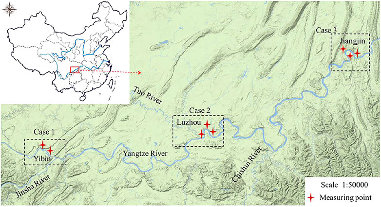
The emission of nitrogen compounds especially like NOx-N nitrates is mainly from the agricultural activities, residents, and industry. The deposition of NOx-N degrades the quality of both groundwater and surface water in regional stream networks. In order to measure the pollutant, the nitrate concentrations in 8 monitoring points in the streams locate in the suburbs of major cities along the Yangtze River are measured on daily basis during the year of 2020. The locations of major cities and the monitoring points which are in the suburbs of these cities are displayed in Figure 1 below.
The dataset collected for this study includes daily contrite concentrations from 8 monitoring points. Meanwhile, the daily discharge volume from surrounding area is also provided. The summary of the dataset has been presented in Table 1. It summarizes the basic statistics including the mean, median, maximum value, minimum value, and standard deviation of the daily nitrate concentrations as well as stream discharge. The unit for the measured nitrate concentration is milligrams per liter (mg L−1) and the unit for the discharge is millimeter (mm) which is mainly from precipitation or groundwater supply.
According to Table 1, daily concentrations of nitrate concentration (NOX-N) ranged from 7.05 to 35.00 mg L−1. Concentrations that exceeded the drinking water standards of 10 mg L−1 for most of the time for almost all monitoring points. This may be exaggerated by the fact that the records in many summer flood seasons are not included for the safety issues during the data collection process. Meanwhile, for 8 monitoring sites, the average daily discharge on days when NOX-N was measured ranged between 1.32 and 1.51 mm during the period of the study. These data also exclude the flood seasons as the observations may be inaccurate and meaningless. Each year, the nitrate concentration varied with discharge during the period of study. Each year, concentrations tend to increase with discharge in a nonlinear fashion.
Abnormal Data Detection
In general, data abnormality is a rarely observed phenomena when some human or systematic errors occur during the measuring process (Gao et al., 2020; Gao et al., 2021). To increase the reliability of the models in our study, we proposed to use “six-sigma” criterion from statistical analysis in our data pre-processing part to detect data abnormality. For a daily nitrate concentration time-series, assumed as
where
Chaotic Modeling of Stream Nitrate Concentration
Dataset Reconstruction
Time-series data representing the daily nitrate concentration usually include dynamic information of the original system. With a certain level of dynamics, the original system is considered as a chaotic system. If the time-series nitrate data are embedded into a higher space, its intrinsic data structure can be reproduced (Ouyang et al., 2020). Hence, reconstruction of the phase space is a valuable solution for modeling chaotic nitrate concentration time series. In general, given the original nitrate concentration time series
where
Temporal Dependency
The time delay
With two discrete nitrate concentration time series defined as
where
where
where
Embedded Dimension
In addition to the time delay, the embedded dimension is another factor affecting the size of the reconstructed phase space. An unsuitable embedded dimension would cause the track of the time series to fold or intersect in the reconstructed phase space. This reflects the number of independent factors that govern the dynamics of the underlying physics system. Only a suitable embedded dimension can ensure that the reconstructed system contains all the independent factors needed to unfold the original system.
In this study, the false nearest neighbors (FNN) method (Bazine & Mabrouki 2019) was adopted to search for the optimal setting for the number of embedded dimensions. It detects the number of neighboring points for different settings of the embedded dimensions repeatedly. If there is no sharp increase with an increase in the number of false neighbors, the embedded dimension increases from m to m+1. Intuitively, the calculations describe variances among false neighbors.
Given two sets of nearest points
Step 1: Compute the distance between the two nearest points using Eq. (6)
where
Step 2: Increase the dimension from m to m+1, and the new distance in the new space can be expressed by Eq. 7 as follows:
Step 3: If the distance between the two nearest points in the new space
where
Lyapunov Exponent
It is seen that the reconstructed data in the new phase space not only retains the original information but also provides more details such as data structures. Hence, studying the chaotic characteristics of the nitrate concentration before data reconstruction is essential.
The Lyapunov exponent is a widely used metric to test whether a system is chaotic or not. It represents the average exponential rates of divergence (expansion) or convergence (contraction) of nearest points in the embedded phase space (Jiang et al., 2021). In general, positive Lyapunov exponent value indicates the presence of chaos and the data structure is unfolded in the reconstructed phase space. If it equals to zero, the system is considered to have bifurcation points or seasonality patterns. Negative values refer to the data points are from stable physics system. Therefore, a positive value of the Lyapunov exponent is needed to demonstrate a phase space is suitable and the reconstructed data is effective to study the original system.
The computation of the Lyapunov exponent can be achieved by applying the approach proposed by Wolf et al. (1985). The process is presented as follows. First, given a start point
In most scenarios, the value of
Echo State Network
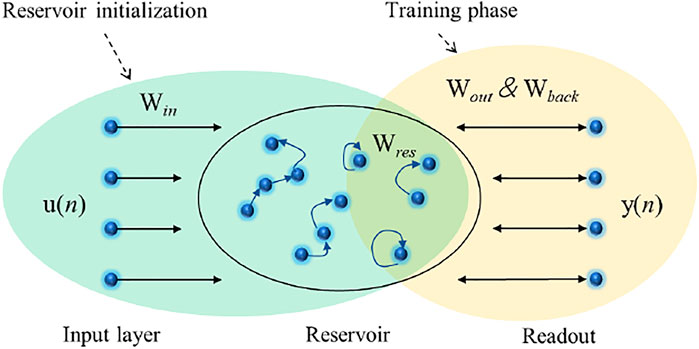
Using the reconstructed data in the new embedded dimension, the day-ahead nitrate concentrations in stream networks were forecasted in this study. Here, the ESN (Chouikhi et al., 2017), which is a deep recurrent neural network, was selected for forecasting. An ESN comprises three layers, namely the input layer, dynamic reservoir, and output payer. Compared with other conventional deep neural networks (DNNs), the ESN contains a dynamic reservoir consisting of several sparsely connected neurons instead of interconnected hidden layers. This structure enables the ESN to have an improved information-processing ability. The architecture of the ESN is shown in Figure 2. Since 2001, ESN has been successfully applied in various fields, including time-series forecasting and classification.
As illustrated in Figure 2, the ESN contains n units in the input layer u, N neurons in the reservoir that form the internal states, and n units in the output layer y. Since this study focuses on day-ahead forecasting of nitrate concentration, the number of units in the output layer y is 1. Assume at time step i, the input state matrix is defined as
where i denotes the number of iterations;
Improved Flower Pollination Algorithm
The setting of hyperparameters of ESN such as reserve layer nodes, reserve layer connection rate, learning rate, and spectral radius all impact the forecasting performance. The improved flower pollination algorithm (IFPA) (Lei et al., 2018), which is based on the principle of biological pollination, has attracted considerable amount of attention in optimizing hyperparameters of deep learning algorithms.
The IFPA algorithm is a swarm intelligence optimization algorithm which contains three major components: cross-pollination, abiotic-pollination and cross-conversion (Li et al., 2021a; Li et al., 2021b). The cross-pollination is a global search strategy which simulates the insects and birds flying under the Levy distribution as in Eq. 12 and 13:
where U obeys the Gaussian distribution
Hence, the updating rules in cross-pollination can be expressed in Eq. 15 as:
Furthermore, the abiotic-pollination is a local searching process and the updating rules is expressed in Eq. 16 as follows:
where
Third, a conversion probability P is introduced to mimic the principle of biological pollination. It controls the conversion of pollen between global pollination and local pollination pollen within iterations. In each iteration, the probability of having global pollination is P and thus the probability of having local pollination is 1-P (Lei et al., 2018; Tang and Zhang, 2019).
Conventional Approaches and Benchmarking Algorithms
To demonstrate the accuracy and effectiveness of the proposed chaotic modeling approach integrated with IFPA-ESN, the comparative analysis is performed in this research against other conventional modeling approach as well as the other benchmarking deep-learning algorithms.
The conventional time-series forecasting approach is based on the autoregression and dependency between residual error and lagged observations. The computation of autocorrelation function (ACF) and PACF (PACF) (Li et al., 2021c) forms the foundations of constructing time-series forecasting approach. The ACF calculates the degree of interaction between current observation and historic lagged observations. PACF helps to determine with its preceding values the correctness degree of current variables while retaining certain constant values. The temporal dependencies as well as the seasonal patterns can be effectively extracted from the dataset. The inputs of the forecasting algorithm can be determined via the computed ACFs and PACFs.
Besides, the temporal signal decomposition gains more popularity in recent publications in short-term forecasting tasks. The main idea is to use temporal signal decomposition algorithms to “break down” a complicated time-series data into simpler and similar series rapidly and efficiently. Then, individual forecasting models can be constructed on each sub-series with improved forecasting accuracy. The Empirical Mode Decomposition (EMD) (Rilling et al., 2003), the Hilbert Vibration Decomposition (HVD) (Sharma and Sharma 2015), and the Variational Mode Decomposition (VMD) (Dragomiretskiy and Zosso 2013) are deemed to be the most representative signal decomposition algorithms used in short-term time-series forecasting tasks. In this research, the VMD is selected for the comparative analysis and it decomposed the complicated nitrate concentration time-series into a finite number of simplified intrinsic mode functions (IMFs). Then the forecasting algorithms are developed based in these IMFs to forecast the short-term values. In the final step, the forecasting results are aggregated to provide the final prediction outcome.
For the benchmarking deep-learning algorithms, the deep neural network (DNN) (Ryu et al., 2017), deep belief network (DBN) (Li et al., 2020), and long short-term memory recurrent neural network (LSTM-RNN) (Kong et al., 2017) are selected to perform the short-term nitrate concentration forecasting tasks with the three modeling approaches as the comparative analysis against the proposed IFPA-ESN. The DNN uses a cascade of multiple layers with nonlinear processing units. It is a fully connected and feedforward network that allows computational models to be composed of multiple processing layers to learn the deep temporal representations in the time-series data. The DBN is consisted of multiple unsupervised restricted Boltzmann machines (RBMs) and a supervised regression layer stacked on the top. Each RBM has a layer of input neurons and a single hidden layer with hidden-to-all-visible connections. Layer-wise training is implemented across multiple RMBs to ensure promising forecasting accuracy. The LSTM-RNN servers as the most widely used state-of-art time-series forecasting algorithms. It is a special type of RNN that is capable to learn long-term and short-term temporal dependencies. Besides, its LSTM blocks contains three gates namely forget gate, input gate, and output gate. These gates make the LSTM blocks smarter than classical neurons and enable them to memorize recent sequences. All selected benchmarking algorithms have demonstrated superior performance in short-term forecasting tasks (He et al., 2017b).
Measurement Metrices
Four measurement metrices are selected to evaluate the performance of the chaotic modeling approach using the IFPA-ESN algorithm including mean absolute error (MAE), mean absolute percentage error (MAPE), root mean square error (RMSE), and hit rate (HR). The definition of the matrices as well as the formulas to compute them are illustrated in Table 2 respectively.
Turning Point Analysis
Parametric Ricker Function
Besides the pollutant concentration forecasting, we also aim to quantify how the discharge regime in the agricultural watershed reflected catchment hydrology and the delivery pathway of nitrate pollutant. The transportation and supply limitations of the nitrogen compounds varies by different locations also (Gao and Meguid 2021). Hence, the turning point analysis is performed in this research to quantify the relation between predicted daily nitrate concentration and stream discharge. In addition, the turning point will be utilized to determine the supply and transport limitations for the case study locations respectively.
Here, the parametric Ricker function (Kirchner et al., 2004) is utilized to model the relationship between daily discharge and predicted nitrate concentration. The Ricker function can be expressed as :
where a>0, b > 0, and c < 0 in most of the cases. It is commonly used to model the hump-shaped data that are skewed to the right such as the discharge-concentration relationship. Since there are measurement errors and the fitted values can vary by measuring time and location, we can further revise the form as Eq. 18 to incorporate our study as follows:
where
Delta Method
In many practical applications, fitting the mean structure of the parametric curve is insufficient. First, in the long-term, the mean structure may vary which brings challenge using only one single parametric function. Second, a slight shift of data points caused by measurement error or extremely high/low discharge would significantly impact the fitted mean structure of the fitted curve. Last, the random errors during the data collection process is inevitable which may complicate the statistical analysis (Toyoda and Wu, 2019; Wu et al., 2020). Hence, in this research, the quantile regression is adopted and the standard errors are also estimated for the parameters as well as the turning points.
The delta method (Jones et al., 2017; Le et al., 2021) is selected to derive the standard errors for the estimated parameters and turning points. First, the natural log is taken on both sides of the Ricker function and it can be expressed in:
Then, the actual discharge data x and predicted nitrate concentration y both can be input into Eq. 19 to derive the estimates of a, b, and c. Then, the turning point is defined to be the x-value for which
where,
In this study, we can derive that for turning point
Experimental Results and Discussion
Data Reconstruction and Modeling
Considering the data homogeneity of nitrate concentration in streams, the daily measured concentrations in 2020 at the eight monitoring points were used for training, validation, and testing. As described in section 3, data reconstruction is helpful for modeling. The mutual information entropy and FNN were applied simultaneously to obtain the optimal parameter settings for data reconstruction. Finally, the Lyapunov exponents, as described in Section 3.4, were utilized to examine whether the reconstructed data using the parameter setting represent a chaotic system.
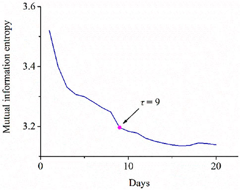
First, the mutual information entropy values were computed for each monitoring point; for example, one of the monitoring points, namely “Yibin-1,” has been illustrated in Figure 3 with respect to the computation of mutual information entropy. The curve depicts the mutual information entropy with respect to time delay in days. It shows an exponentially decaying pattern, which indicates that the relevance of the two series weakens with an increase in the delay times. For convenience, the optimal time delay is usually selected when the value of the mutual information reaches its first local minimum value. Hence, in the example shown in Figure 3, the delay time of the nitrate concentration is set as 9. The time delay τ values for all monitoring points are computed and summarized in Table 3.
Meanwhile, the minimum embedded dimensions m for the monitoring points were computed using the FNN method while taking the computed time delay τ values as a prerequisite. Here, we set the value of the threshold to
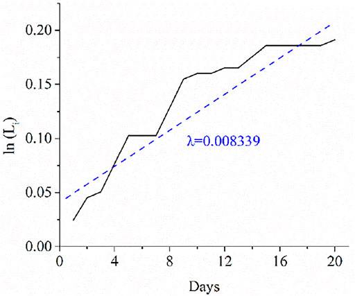
In addition, the Lyapunov exponents were computed to determine whether the reconstructed time-series system is chaotic. As shown in Figure 4, the reconstructed nitrate concentration data in “Yibing-1” location was measured for the Lyapunov exponent λ. It was calculated using the slope coefficient between ln L and T. If λ is positive (i.e., λ > 0 in Figure 4), the system is chaotic, and the reconstructed time series is unfolded, as described in Sections 3.3 and 3.4. The computed λ values for all the eight monitoring points are summarized in Table 3.
Prediction Based on Chaotic Modeling
Furthermore, a comparative analysis was performed against the traditional time-series forecasting approach and the temporal signal decomposition forecasting approach. In each approach, the proposed IFPA-ESN algorithm was compared with the other benchmarking deep learning algorithms listed in Section 3.7 above.
First, the IFPA optimization algorithm was used to optimize the hyperparameters of the ESN network. The reserve layer nodes, reserved layer connection rate, learning rate, and spectral radius were optimized simultaneously. Four benchmark functions, namely sphere, Rastrigin, Ackley, and Schaffer, were selected and compared. The benchmarking functions are all “landscape generator” class, and the differences among the functions relate to the number of minima within the search space, general convergence rate to the global optimal, and additional harmonic potential outside the search space to force the solution to stay within the boundaries. For each function, we performed a maximum of 2000 iterations for each experiment, and a total of 20 experiments were conducted. The performances of the four functions are summarized in Table 4.
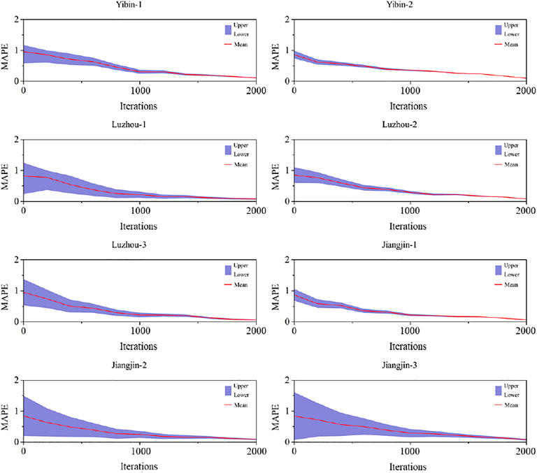
As shown in Table 4, MIN, MAX, and Average denote the minimum, maximum, and average MAPEs, respectively, per iteration for the 20 experiments performed. CR refers to the convergence rate, which is the overall probability that the algorithm can converge to the default minimum value using benchmark functions. From Table 4, it can be inferred that the Schaffer function has the smallest mean iterations of convergence compared with the others. In addition, the convergence rate of the Schaffer function is the highest, which implies the largest probability of reaching the default minimum value of the loss function. Hence, the Schaffer function was selected as the default function for the IFPA algorithm. Using the Schaffer function, the mean MAPEs and the upper/lower bounds of the 95% confidence interval were computed in each iteration. The convergence measured using the MAPE for each monitoring point is illustrated in Figure 5.
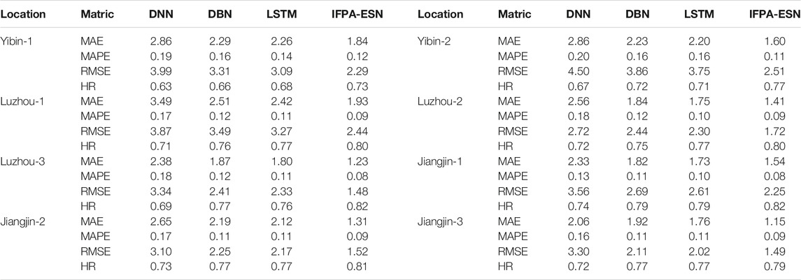
Next, to demonstrate the performance of the proposed chaotic modeling approach using IFPA-ESN, two other modeling approaches, conventional time-series forecasting and temporal signal decomposition, were applied and compared. The time-series forecasting approach was based on computation of the ACF and PACF values for each monitoring point. The temporal dependencies and seasonality were considered in the modeling approach. In the signal decomposition approach, the time-series nitrate concentrations were decomposed into nine simplified intrinsic mode functions (IMFs). For each IMF, a short-term forecasting sub-model was constructed. The final forecasting results were the aggregation of all forecasting outcomes produced by the nine sub-models.
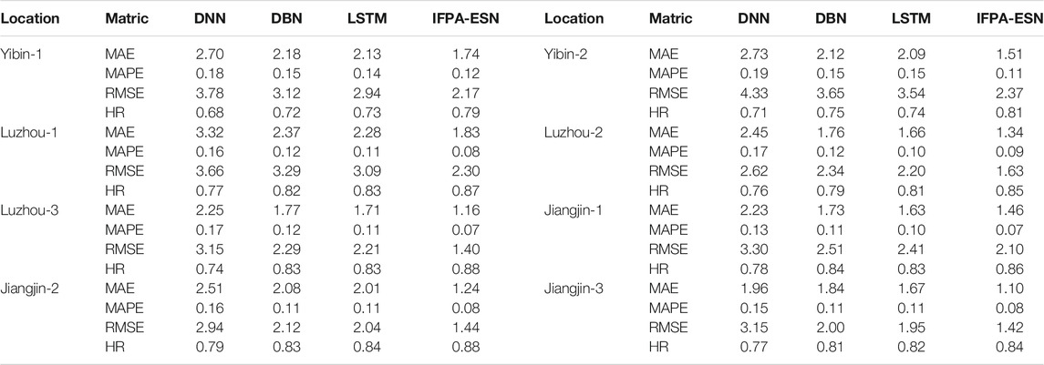
Table 5 summarizes the forecasting performance over the testing dataset of all the deep learning algorithms tested, as described in Section 3.7. Using a conventional time-series forecasting approach, the proposed IFPA-ESN outperformed all the other benchmarking algorithms tested. The forecasting performances of all the algorithms tested using the signal decomposition approach are presented in Table 6. The proposed IFPA-ESN provided the smallest MAE, MAPE, and RMSE values. Meanwhile, it provided the highest values of HR, which demonstrates its superior power in short-term nitrate concentration forecasting.
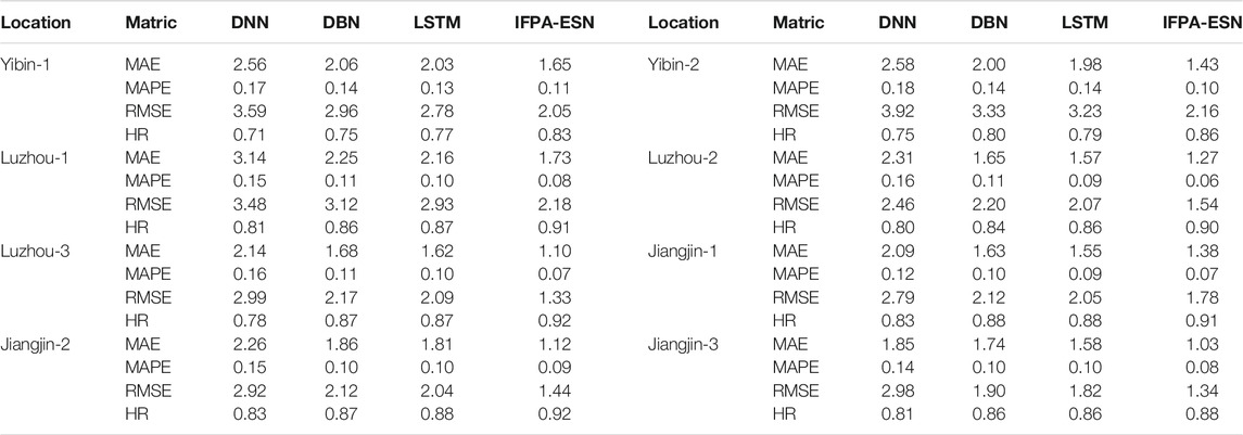
The global performance of short-term nitrate concentrations obtained using the chaotic modeling approach is summarized in Table 7. IFPA-ESN still outperformed all the algorithms tested in this scenario. In addition, for all the tested algorithms, the chaotic modeling approach had fewer forecasting errors, which validated its superior power in discovering the real data structure. The forecasting outcomes of the testing dataset and the observed actual nitrate concentrations are shown in Figure 6.
Discussion of the Turning Points
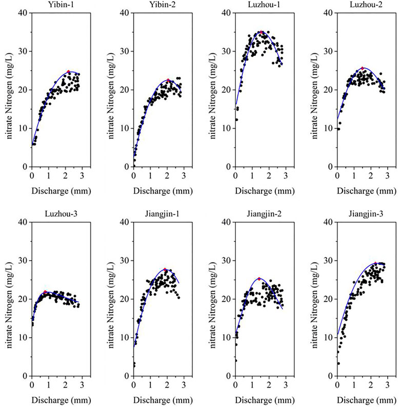
The forecasted nitrate concentration in the testing dataset (100 days) integrated with the measured stream discharge during the same period was utilized for turning point analysis. Here, the forecasted daily concentration versus discharge data at the same monitoring location is provided. An examination of the turning point analysis, as described in Section 4, was performed, and the results are summarized and illustrated in Table 8 and Figure 7.
Table 8 presents results of the fitted Ricker function using the quantile regression. The turning points were also computed with the standard errors provided. As shown in Table 8, the turning points varied from 0.79 to 2.27 mm depending on the measured stream location, which is impacted by drought. The standard errors were computed using the Delta’s method, and the values varied between 0.05 and 0.14 mm. Considering the estimated turning points, the standard errors were within a small range, which indicated the reliability of the estimation.
The fitted Ricker function is plotted in Figure 7. It depicts the nonlinear relationship between the forecasted nitrate concentrations and the stream discharges. The turning points are labeled in red in Figure 7, and the fitted Ricker function is plotted as a blue curve. At each monitoring point, the nitrate concentration started to decline as the discharge exceeded the turning point. This supports the idea that drought impacts stream nitrate concentrations in the temporal domain.
Table 9 summarizes the delineation between transport- and supply-limited days. Based on the percentages of loads before the turning point, the locations such as Yibin-1, Yibin-2, Luzhou-1, Luzhou-2, Luzhou-3, and Jiangjin-1 are transport limited. Only two locations, namely Jiangjin-2 and Jiangjin-3, are supply limited. The proportion of loads before the turning points varied between 53 and 81% under the transport-limited condition. It is noteworthy that the proportion of loads before the turning points was between 41 and 42% under supply-limited conditions. These conditions indicate that supply considerations are likely to control the flux of NOx-N in stream networks.
Conclusion
In this study, insights are provided for experts, academicians, and officers of local environment protection agencies via chaotic modeling of stream nitrate concentrations using IFPA-ESN. This study also provides a turning point analysis to quantify nitrate concentration-discharge relations. In addition, the limitations of pollutant transport and supply patterns were estimated in all case studies.
The computational results revealed that IFPA-ESN integrated with a chaotic modeling strategy achieved a satisfactory level of accuracy for forecasting the daily nitrate concentration in stream networks using historical time-series data. Compared with other time-series modeling scenarios, the chaotic modeling strategy demonstrated superior performance in terms of forecasting accuracy. Meanwhile, the hyperparameters of the ESN were carefully tuned or searched to reach the optimal setting using the IFPA algorithm. The IFPA-ESN provided peak forecasting performances comparable to those of other benchmarking machine-learning and deep learning algorithms in our eight case study locations. On the other hand, the turning point analysis using parametric Ricker functions accurately fitted the trend of nonlinear relations between nitrate concentration and discharge in eight case study locations. Furthermore, the delineation between transport and supply limitations was discussed to gain insights into nitrate pollution in stream systems.
Future recommendations include incorporating various climate-related external factors into the decision-making process in the light of further reduction in forecasting volatility; these external factors include precipitation, ambient temperature, wind speed, air humidity, and soil-water relationships. Moreover, future studies should aim to develop federated learning systems to incorporate the deep learning-based chaotic modeling strategy to forecast nitrate pollution simultaneously for multiple locations while protecting data privacy.
Data Availability Statement
The raw data supporting the conclusions of this article will be made available by the authors, without undue reservation.
Author Contributions
YT conceptualized the study, contributed to the study methodology, and wrote the original draft. JD contributed to the study methodology, data curation and investigation. CZ contributed to software and formal analysis. QW contributed to editing and data curation. All authors have read and agreed to the published version of the manuscript.
Funding
This work was supported by the Regional Innovation Cooperation Programs of Sichuan province (2021YFQ0050).
Conflict of Interest
The authors declare that the research was conducted in the absence of any commercial or financial relationships that could be construed as a potential conflict of interest.
Publisher’s Note
All claims expressed in this article are solely those of the authors and do not necessarily represent those of their affiliated organizations, or those of the publisher, the editors, and the reviewers. Any product that may be evaluated in this article, or claim that may be made by its manufacturer, is not guaranteed or endorsed by the publisher.
References
Ahmad, T., Zhang, D., and Huang, C. (2021). Methodological Framework for Short-And Medium-Term Energy, Solar and Wind Power Forecasting with Stochastic-Based Machine Learning Approach to Monetary and Energy Policy Applications. Energy 231, 120911. doi:10.1016/j.energy.2021.120911
Bazine, H., and Mabrouki, M. (2019). Chaotic Dynamics Applied in Time Prediction of Photovoltaic Production. Renew. Energ. 136, 1255–1265. doi:10.1016/j.renene.2018.09.098
Belitz, K., Fram, M. S., and Johnson, T. D. (2015). Metrics for Assessing the Quality of Groundwater Used for Public Supply, CA, USA: Equivalent-Population and Area. Environ. Sci. Technol. 49 (14), 8330–8338. doi:10.1021/acs.est.5b00265
Blesh, J., and Drinkwater, L. E. (2013). The Impact of Nitrogen Source and Crop Rotation on Nitrogen Mass Balances in the Mississippi River Basin. Ecol. Appl. 23 (5), 1017–1035. doi:10.1890/12-0132.1
Chouikhi, N., Ammar, B., Rokbani, N., and Alimi, A. M. (2017). PSO-based Analysis of Echo State Network Parameters for Time Series Forecasting. Appl. Soft Comput. 55, 211–225. doi:10.1016/j.asoc.2017.01.049
Cui, S., Pei, X., Jiang, Y., Wang, G., Fan, X., Yang, Q., et al. (2021). Liquefaction within a Bedding Fault: Understanding the Initiation and Movement of the Daguangbao Landslide Triggered by the 2008 Wenchuan Earthquake (Ms = 8.0). Eng. Geology. 295, 106455. doi:10.1016/j.enggeo.2021.106455
David, M. B., Gentry, L. E., Kovacic, D. A., and Smith, K. M. (1997). Nitrogen Balance in and export from an Agricultural Watershed. Am. Soc. Agron. Crop Sci. Soc. America, Soil Sci. Soc. America 26 (No. 4), 1038–1048. doi:10.2134/jeq1997.00472425002600040015x
Domangue, R. J., and Mortazavi, B. (2018). Nitrate Reduction Pathways in the Presence of Excess Nitrogen in a Shallow Eutrophic Estuary. Environ. Pollut. 238, 599–606. doi:10.1016/j.envpol.2018.03.033
Dragomiretskiy, K., and Zosso, D. (2013). Variational Mode Decomposition. IEEE Transactions Signal. Processing 62 (3), 531–544.
Gao, G., and Meguid, M. A. (2021). On the Role of Joint Roughness on the Micromechanics of Rock Fracturing Process: a Numerical Study. Acta Geotechnica, 1–26. doi:10.1007/s11440-021-01401-8
Gao, G., Meguid, M. A., Chouinard, L. E., and Xu, C. (2020). Insights into the Transport and Fragmentation Characteristics of Earthquake-Induced Rock Avalanche: Numerical Study. Int. J. Geomech. 20 (9), 04020157. doi:10.1061/(asce)gm.1943-5622.0001800
Gao, G., Meguid, M. A., Chouinard, L. E., and Zhan, W. (2021). Dynamic Disintegration Processes Accompanying Transport of an Earthquake-Induced Landslide. Landslides 18 (3), 909–933. doi:10.1007/s10346-020-01508-1
He, Y., Deng, J., and Li, H. (2017b). “Short-term Power Load Forecasting with Deep Belief Network and Copula Models,” in 9th International conference on intelligent human-machine systems and cybernetics (IHMSC), IEEE. 1, 191–194. doi:10.1109/ihmsc.2017.50
He, Y., Kusiak, A., Ouyang, T., and Teng, W. (2017a). Data-driven Modeling of Truck Engine Exhaust Valve Failures: a Case Study. J. Mech. Sci. Technol. 31 (6), 2747–2757. doi:10.1007/s12206-017-0518-1
He, Y., and Kusiak, A. (2018). Performance Assessment of Wind Turbines: Data-Derived Quantitative Metrics. IEEE Trans. Sustain. Energ. 9 (1), 65–73. doi:10.1109/tste.2017.2715061
Hrnjica, B., Mehr, A. D., Jakupović, E., Crnkić, A., and Hasanagić, R. (2021). “Application of Deep Learning Neural Networks for Nitrate Prediction in the Klokot River, Bosnia and Herzegovina,” in 2021 7th International Conference on Control, Instrumentation and Automation (ICCIA) (IEEE), 1–6. February.
Hu, Q., Zhang, R., and Zhou, Y. (2016). Transfer Learning for Short-Term Wind Speed Prediction with Deep Neural Networks. Renew. Energ. 85, 83–95. doi:10.1016/j.renene.2015.06.034
Huang, G.-B., Wang, D. H., and Lan, Y. (2011). Extreme Learning Machines: a Survey. Int. J. Mach. Learn. Cyber. 2 (2), 107–122. doi:10.1007/s13042-011-0019-y
Jiang, J., Tang, S., Liu, R., Sivakumar, B., Wu, X., and Pang, T. (2021). A Hybrid Wavelet-Lyapunov Exponent Model for River Water Quality Forecast. J. Hydroinformatics 23 (4), 864–878. doi:10.2166/hydro.2021.023
Jones, C. S., Wang, B., Schilling, K. E., and Chan, K.-s. (2017). Nitrate Transport and Supply Limitations Quantified Using High-Frequency Stream Monitoring and Turning point Analysis. J. Hydrol. 549, 581–591. doi:10.1016/j.jhydrol.2017.04.041
Keupers, I., and Willems, P. (2017). Development and Testing of a Fast Conceptual River Water Quality Model. Water Res. 113, 62–71. doi:10.1016/j.watres.2017.01.054
Kirchner, J. W., Feng, X., Neal, C., and Robson, A. J. (2004). The fine Structure of Water-Quality Dynamics: The(high-Frequency) Wave of the Future. Hydrol. Process. 18 (7), 1353–1359. doi:10.1002/hyp.5537
Kong, W., Dong, Z. Y., Jia, Y., Hill, D. J., Xu, Y., and Zhang, Y. (2017). Short-term Residential Load Forecasting Based on LSTM Recurrent Neural Network. IEEE Trans. Smart Grid 10 (1), 841–851.
Le, S., Wu, Y., Guo, Y., and Del Vecchio, C. (2021). “Game Theoretic Approach for a Service Function Chain Routing in NFV with Coupled Constraints,” in IEEE Transactions on Circuits and Systems II: Express Briefs. doi:10.1109/tcsii.2021.3070025
LeCun, Y., and Bengio, Y. (1995). Convolutional Networks for Images, Speech, and Time Series. The handbook Brain Theor. Neural networks 3361 (10), 1995.
Lei, X., Fang, M., Wu, F. X., and Chen, L. (2018). Improved Flower Pollination Algorithm for Identifying Essential Proteins. BMC Syst. Biol. 12 (4), 46–140. doi:10.1186/s12918-018-0573-y
Li, H., Deng, J., Feng, P., Pu, C., Arachchige, D. D. K., and Cheng, Q. (2021a). Short-Term Nacelle Orientation Forecasting Using Bilinear Transformation and ICEEMDAN Framework. Front. Energ. Res. 9, 780928. doi:10.3389/fenrg.2021.780928
Li, H., Deng, J., Yuan, S., Feng, P., and Arachchige, D. D. K. (2021b). Monitoring and Identifying Wind Turbine Generator Bearing Faults Using Deep Belief Network and EWMA Control Charts. Front. Energ. Res. 9, 799039. doi:10.3389/fenrg.2021.799039
Li, H., He, Y., Xu, Q., Deng, J., Li, W., and Wei, Y. (2022). Detection and Segmentation of Loess Landslides via Satellite Images: a Two-phase Framework. Landslides, 1–14. doi:10.1007/s10346-021-01789-0
Li, H., Xu, Q., He, Y., and Deng, J. (2018). Prediction of Landslide Displacement with an Ensemble-Based Extreme Learning Machine and Copula Models. Landslides 15 (10), 2047–2059. doi:10.1007/s10346-018-1020-2
Li, H., Xu, Q., He, Y., Fan, X., and Li, S. (2020). Modeling and Predicting Reservoir Landslide Displacement with Deep Belief Network and EWMA Control Charts: a Case Study in Three Gorges Reservoir. Landslides 17 (3), 693–707. doi:10.1007/s10346-019-01312-6
Li, H., Xu, Q., He, Y., Fan, X., Yang, H., and Li, S. (2021c). Temporal Detection of Sharp Landslide Deformation with Ensemble-Based LSTM-RNNs and Hurst Exponent. Geomatics, Nat. Hazards Risk 12 (1), 3089–3113. doi:10.1080/19475705.2021.1994474
Nolan, B. T., Gronberg, J. M., Faunt, C. C., Eberts, S. M., and Belitz, K. (2014). Modeling Nitrate at Domestic and Public-Supply Well Depths in the Central Valley, California. Environ. Sci. Technol. 48 (10), 5643–5651. doi:10.1021/es405452q
Ostad-Ali-Askari, K., Shayannejad, M., and Ghorbanizadeh-Kharazi, H. (2017). Artificial Neural Network for Modeling Nitrate Pollution of Groundwater in Marginal Area of Zayandeh-Rood River, Isfahan, Iran. KSCE J. Civ Eng. 21 (1), 134–140. doi:10.1007/s12205-016-0572-8
Ouyang, T., Cha, X., and Qin, L. (2016). Medium-or Long-Term Wind Power Prediction with Combined Models of Meteorological Multi-Variables. Power Syst. Tech. 40 (03), 847–852.
Ouyang, T., He, Y., and Huang, H. (2018). Monitoring Wind Turbines' Unhealthy Status: a Data-Driven Approach. IEEE Trans. Emerging Top. Comput. Intelligence 3 (2), 163–172.
Ouyang, T., He, Y., Li, H., Sun, Z., and Baek, S. (2019a). Modeling and Forecasting Short-Term Power Load with Copula Model and Deep Belief Network. IEEE Trans. Emerg. Top. Comput. Intell. 3 (2), 127–136. doi:10.1109/tetci.2018.2880511
Ouyang, T., Huang, H., He, Y., and Tang, Z. (2020). Chaotic Wind Power Time Series Prediction via Switching Data-Driven Modes. Renew. Energ. 145, 270–281. doi:10.1016/j.renene.2019.06.047
Ouyang, T., Zha, X., Qin, L., He, Y., and Tang, Z. (2019b). Prediction of Wind Power Ramp Events Based on Residual Correction. Renew. Energ. 136, 781–792. doi:10.1016/j.renene.2019.01.049
Ransom, K. M., Nolan, B. T., A. Traum, J., Faunt, C. C., Bell, A. M., Gronberg, J. A. M., Wheeler, D. C., Z. Rosecrans, C., Jurgens, B., Schwarz, G. E., Belitz, K., M. Eberts, S., Kourakos, G., and Harter, T. (2017). A Hybrid Machine Learning Model to Predict and Visualize Nitrate Concentration throughout the Central Valley Aquifer, California, USA. Sci. Total Environ. 601-602, 1160–1172. doi:10.1016/j.scitotenv.2017.05.192
Rilling, G., Flandrin, P., and Goncalves, P. (2003). “June). On Empirical Mode Decomposition and its Algorithms,” in IEEE-EURASIP Workshop on Nonlinear Signal and Image Processing, 3, 8–11. NSIP-03, Grado (I).3
Rosenstein, M. T., Collins, J. J., and De Luca, C. J. (1994). Reconstruction Expansion as a Geometry-Based Framework for Choosing Proper Delay Times. Physica D: Nonlinear Phenomena 73 (1-2), 82–98. doi:10.1016/0167-2789(94)90226-7
Ryu, S., Noh, J., and Kim, H. (2017). Deep Neural Network Based Demand Side Short Term Load Forecasting. Energies 10 (1), 3.
Sajedi-Hosseini, F., Malekian, A., Choubin, B., Rahmati, O., Cipullo, S., Coulon, F., et al. (2018). A Novel Machine Learning-Based Approach for the Risk Assessment of Nitrate Groundwater Contamination. Sci. total Environ. 644, 954–962. doi:10.1016/j.scitotenv.2018.07.054
Sharma, H., and Sharma, K. K. (2015). Baseline Wander Removal of ECG Signals Using Hilbert Vibration Decomposition. Electron. Lett. 51 (6), 447–449. doi:10.1049/el.2014.4076
Shi, P., Zhang, Y., Song, J., Li, P., Wang, Y., Zhang, X., Li, Z., Bi, Z., Zhang, X., Qin, Y., and Zhu, T. (2019). Response of Nitrogen Pollution in Surface Water to Land Use and Social-Economic Factors in the Weihe River Watershed, Northwest China. Sustain. Cities Soc. 50, 101658. doi:10.1016/j.scs.2019.101658
Stamenković, L. J., Mrazovac Kurilić, S., and Presburger Ulniković, V. (2020). Prediction of Nitrate Concentration in Danube River Water by Using Artificial Neural Networks. Water Supply 20 (6), 2119–2132.
Tang, Z., and Zhang, Z. (2019). The Multi-Objective Optimization of Combustion System Operations Based on Deep Data-Driven Models. Energy 182, 37–47. doi:10.1016/j.energy.2019.06.051
Tang, Z., Zhao, G., and Ouyang, T. (2021). Two-phase Deep Learning Model for Short-Term Wind Direction Forecasting. Renew. Energ. 173, 1005–1016. doi:10.1016/j.renene.2021.04.041
Toyoda, M., and Wu, Y. (2019). Mayer-type Optimal Control of Probabilistic Boolean Control Network with Uncertain Selection Probabilities. IEEE Trans. cybernetics 51 (6), 3079–3092. doi:10.1109/tcyb.2019.2954849
Villarini, G., Jones, C. S., and Schilling, K. E. (2016). Soybean Area and Baseflow Driving Nitrate in Iowa's Raccoon River. J. Environ. Qual. 45 (6), 1949–1959. doi:10.2134/jeq2016.05.0180
Wolf, A., Swift, J. B., Swinney, H. L., and Vastano, J. A. (1985). Determining Lyapunov Exponents from a Time Series. Physica D: nonlinear phenomena 16 (3), 285–317. doi:10.1016/0167-2789(85)90011-9
Wu, Y., Guo, Y., and Toyoda, M. (2020). “Policy Iteration Approach to the Infinite Horizon Average Optimal Control of Probabilistic Boolean Networks,” in IEEE Transactions on Neural Networks and Learning Systems.
Xu, Q., Li, H., He, Y., Liu, F., and Peng, D. (2019). Comparison of Data-Driven Models of Loess Landslide Runout Distance Estimation. Bull. Eng. Geol. Environ. 78 (2), 1281–1294. doi:10.1007/s10064-017-1176-3
Zhang, Y., Shi, P., Li, F., Wei, A., Song, J., and Ma, J. (2018). Quantification of Nitrate Sources and Fates in Rivers in an Irrigated Agricultural Area Using Environmental Isotopes and a Bayesian Isotope Mixing Model. Chemosphere 208, 493–501. doi:10.1016/j.chemosphere.2018.05.164
Keywords: nitrate concentration, chaotic system, improved flower pollination optimization, echo state network, turning point analysis
Citation: Tang Y, Deng J, Zang C and Wu Q (2022) Chaotic Modeling of Stream Nitrate Concentration and Transportation via IFPA-ESN and Turning Point Analyses. Front. Environ. Sci. 10:855694. doi: 10.3389/fenvs.2022.855694
Received: 15 January 2022; Accepted: 04 February 2022;
Published: 04 March 2022.
Edited by:
Jingren Zhou, Sichuan University, ChinaReviewed by:
Ge Gao, McGill University, CanadaTinghui Ouyang, National Institute of Advanced Industrial Science and Technology (AIST), Japan
Copyright © 2022 Tang, Deng, Zang and Wu. This is an open-access article distributed under the terms of the Creative Commons Attribution License (CC BY). The use, distribution or reproduction in other forums is permitted, provided the original author(s) and the copyright owner(s) are credited and that the original publication in this journal is cited, in accordance with accepted academic practice. No use, distribution or reproduction is permitted which does not comply with these terms.
*Correspondence: Jiahao Deng, amRlbmc1QGRlcGF1bC5lZHU=
 Yandong Tang1
 Jiahao Deng