 Elizabeth A. Meier
 Peter J. Thorburn
 Lindsay W. Bell
 Matthew T. Harrison
 Jody S. Biggs
- 1Agriculture and Food, Commonwealth Scientific and Industrial Research Organisation, St Lucia, QLD, Australia
- 2Agriculture and Food, Commonwealth Scientific and Industrial Research Organisation, Toowoomba, QLD, Australia
- 3School of Land and Food, Tasmanian Institute of Agriculture, University of Tasmania, Burnie, TAS, Australia
The agricultural sector has potential to provide greenhouse gas (GHG) mitigation by sequestering soil organic carbon (SOC). Replacing cropland with permanent pasture is one practice promoted for its potential to sequester soil carbon. However, pastures frequently support livestock, which produce other GHG emissions that could negate the abatement from increased SOC, especially given the declining rate of SOC sequestration through time. Our purpose was to determine whether the abatement provided by SOC storage in permanent pastures was offset by livestock emissions, and to thus compare emissions from grazed pasture systems with those from cropping systems. We investigated this question for three case study farms in locations with contrasting climate, soils and management representative of Australian cropping and livestock systems. Three cropping scenarios were defined that had increasing amounts of SOC inputs: Cropburn, crop residues burned before sowing (lowest SOC input); Cropstubble, crop residues retained; and Cropintensity, uncropped fallow phases replaced with short-term green manure legume crops. The on-farm GHG emissions profiles of these cropping scenarios were compared with those from two livestock scenarios utilizing continuous stocking: Livestockgrass, stocked permanent grass pasture; and Livestocklegume, stocked permanent legume pasture; the latter having higher SOC input than the former. Crop yields, pasture growth rates and emissions of carbon dioxide (CO2) and nitrous oxide (N2O) from the soil were simulated with the APSIM farming systems model. Livestock emissions were predicted using Australian GHG accounting emission factors. For the farms in this study, the SOC sequestered in the stocked permanent pastures was offset by emissions from livestock, and emissions from cropping scenarios were similar to or significantly less than those from the livestock scenarios. These findings: (1) demonstrate the importance of using net GHG abatement potentials from combined emissions rather than a single GHG abatement process when evaluating potential abatement practices, and (2) demonstrate that characteristics of different locations can alter the abatement potential of management practices.
Introduction
The “Agriculture, Forestry and Other Land Use (AFOLU)” economic sector emits 24.8% of global greenhouse gases (GHGs), including 0.5 Gt carbon dioxide equivalents (CO2e) yr−1 from enteric fermentation and 1.2 Gt CO2e yr−1 from agricultural soils (Smith et al., 2014). The principal emissions from agricultural practices consist of (1) carbon dioxide (CO2) from decomposition of soil organic carbon (SOC), (2) methane (CH4) from enteric fermentation, and (3) nitrous oxide (N2O) from synthetic fertilizer and manure [DEE (Department of the Environment and Energy), 2014, 2016; Smith et al., 2014]. The global warming potential (GWP) of each gas differs, however, with CO2e values of 3.7, 34, and 298 for SOC, CH4, and N2O, respectively (IPCC, 2013). Thus, the potential for abatement in different agricultural systems depends on both the GWP and volume of the greenhouse gas emitted.
Agricultural GHG emissions from changes in SOC stocks, N2O, and CH4 are highly variable across environments and management practices (e.g., Hillier et al., 2012; Sainju, 2016). The balance between SOC decomposition and sequestration is influenced by the amount and nature of carbon inputs (e.g., through stubble retention, manure application and cover crops; Lal, 2004; Sanderman et al., 2010; Luo et al., 2011; Wang et al., 2016) and environmental conditions influencing the rate of SOC decomposition (e.g., Badgery et al., 2013). Emissions of N2O from soils are stimulated by warm temperatures, high water contents, and a supply of nitrate and decomposable carbon (Dalal et al., 2003). Accordingly, the potential for changes in both SOC stocks and N2O emissions are influenced by rainfall, temperature, management practices, and soil properties. By comparison, emissions of CH4 are primarily determined by stocking rate (Harrison et al., 2014b), and flock/herd structure and feed composition (Hegarty et al., 2010; Harrison et al., 2014a; Henderson et al., 2017). Thus, the diversity of factors that influence emissions of individual GHGs can make it difficult to identify practices that deliver overall mitigation.
Despite the relatively small GWP of CO2, abatement practices that increase SOC are desirable because of their unique potential among agricultural practices to sequester (rather than merely reduce emissions of) atmospheric GHGs (Smith et al., 2014). Increasing the amount of carbon sequestered in soils has the potential to halt the annual increase in CO2 in the atmosphere and thus mitigate climate change (e.g., the 4 per 1,000 Initiative; http://4p1000.org/understand). The inclusion of pastures in agricultural systems is an effective method to maximize SOC sequestration due to high carbon inputs from pasture (Parsons et al., 2009; Luo et al., 2010; Stockmann et al., 2013; Lugato et al., 2015). Thus, in cropping systems, temporary (e.g., 2–5 year) pasture phases within cropping rotations increase SOC (Sanderman et al., 2010; Luo et al., 2011; Rabbi et al., 2014; Murphy, 2015). However, these gains are progressively “lost” as SOC mineralizes during subsequent cropping phases (Bell and Lawrence, 2009; Mielenz et al., 2017). Conversion of cropping land to permanent pastures results in longer term increases in SOC (Franzluebbers et al., 2000; Franzluebbers and Stuedemann, 2009; Bell et al., 2012; Schwenke et al., 2013), although the rate of SOC sequestration declines over time. In addition, because C and N cycles are linked, the increased SOC provides additional substrate (i.e., decomposable carbon) that could increase N2O emissions (Li et al., 2005; Barton et al., 2016), potentially reducing the net extent of GHG abatement provided by SOC sequestration under pastures. Further, pastures usually support ruminant animals (de Boer et al., 2011; Bell and Moore, 2012; Meyer et al., 2016), which produce additional emissions of CH4 and N2O from enteric fermentation, manure and urine, again reducing the net GHG abatement from pastures. Thus, it is difficult to judge the extent of GHG abatement provided by permanent, grazed pastures compared with the cropping systems they might replace.
There are few studies that compare GHG emissions from permanent pastures supporting livestock with those from cropping systems. Abatement from SOC sequestration in permanent pastures supporting livestock can partially (Crosson et al., 2011) or completely (Rutledge et al., 2015; Meyer et al., 2016) offset the emissions from livestock for up to two decades. However, as SOC concentrations approach equilibrium in the longer term, net emissions are likely to increase as CH4 emissions from livestock systems dominate the GHG balances of the fields (Crosson et al., 2011). Thus, the field-scale GHG emissions of cropping systems compared with stocked permanent pastures is unclear. To address the knowledge gap, we investigated the long-term net GHG abatement of stocked permanent pastures relative to cropping systems at three contrasting locations in Australia.
Methods
Case Study Farms
Three case study farms in the Australian mixed crop-livestock zone were defined in collaboration with the farm owners and their advisors (Table 1). The farms were selected from locations where crop-livestock integration is common, and which represented diverse soils and climates. Soil properties were based on measurements of the soils when sampled during previous soil characterization activities at the farms (the ApSoil database; Dalgliesh et al., 2012). Soil profiles described in ApSoil are typically obtained at a single point in time from farms that participate in agricultural studies. Historical land use information was not available but was likely to be a mix of cropping interspersed with short periods of pasture typical in these areas. Rainfall and temperature data were obtained from daily historical climate records obtained from the SILO data base (Jeffrey et al., 2001) for weather stations close to the case study farms (Figure 1).
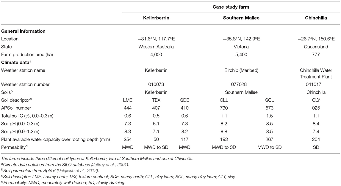
Table 1. Location and soils information for the Kellerberrin, Southern Mallee, and Chinchilla case study farms.
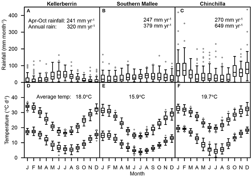
Figure 1. Monthly rainfall (A–C) and minimum and maximum daily temperature (D–F) for the period 1954–2013 recorded in the climate files used to simulate the Kellerberrin, Southern Mallee, and Chinchilla case study farms. Plots show the median, 25 and 75th percentiles in the box, with 1.5 times the interquartile range in the whiskers and outliers shown as symbols.
The Kellerberrin and Southern Mallee case study farms were located in southern Australia and had Mediterranean climates (Table 1; Figure 1). Cropping activities for these locations are typically restricted to the April-October growing season. Soils at the Kellerberrin farm were predominantly sandy and well-drained. In comparison, soils at the Southern Mallee had well-drained sandy surface soils overlying less permeable clayey subsoils. The soils were assumed to be equally represented within each farm.
The Chinchilla farm had strongly contrasting climate and soil properties to the other two case study farms (Table 1; Figure 1). This farm was located in a subtropical environment with summer-dominant rainfall. Average rainfall at the farm was approximately double that received at the other two case study farms. Soils on the farm were cracking clays that had large water holding capacity. The soil water holding capacity and higher rainfall at the Chinchilla farm allow both summer and winter crops to be grown.
Crop and Livestock Simulation Scenarios
Three cropping and two livestock scenarios were simulated that provided a range of potential GHG abatement. For cropping systems (described in more detail in section Crops and Management) this included (1) the usual cropping system at the farms with 70% of stubble removed by burning at the end of March (Cropburn) or (2) a system with stubble retained after harvest (Cropstubble) that had higher GHG abatement potential. A third, high organic matter input cropping scenario was modeled in which all weedy pasture phases and uncropped fallows (Table 2) were replaced with a green manure legume crop (Cropintensity). The green manure crop was sown after harvest of the preceding cash crop and was not fertilized with N. After 60 days the green manure crop was sprayed out and the residues were retained on the soil surface. The two livestock system scenarios (described in more detail in sections Pastures and Management and Defining Livestock Dynamics With the Feed Demand Calculator) consisted of permanent pastures of (1) grass fertilized with N (Livestockgrass) and (2) a legume pasture that was not fertilized with N (Livestocklegume) and stocked at a higher rate. The Cropburn, Cropstubble, and Cropintensity scenarios for crop systems, and the Livestockgrass and Livestocklegume scenarios for livestock systems, were set up with the expectation of having increasing dry matter production and therefore of increasing inputs of SOC to those systems.
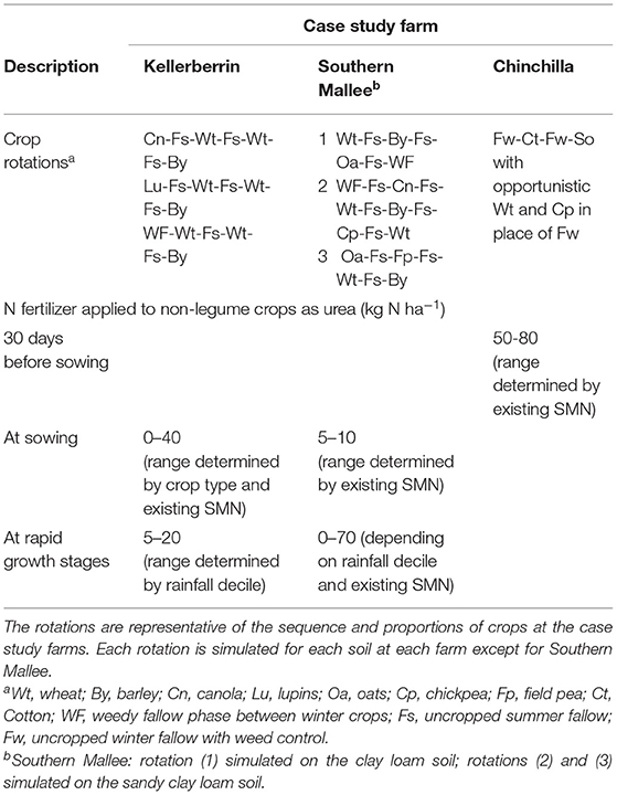
Table 2. Crop rotations and the range of nitrogen fertilizer typically applied, at the Kellerberrin, Southern Mallee, and Chinchilla case study farms.
Overview of Approach for Simulating Crop and Livestock Scenarios
Cropping Systems
GHG emissions from SOC, N2O, and CH4 are determined by the interaction of many factors, so a simulation-based approach was used in this study because it allowed the trade-offs between GHGs to be examined as a system with common conditions and over the long-term (Moore, 2014; Moore et al., 2015). The approach adopted to simulate GHGs from the cropping systems defined for the case study farms is summarized in Figure 2. The cropping systems were simulated with the Agricultural Production Systems sIMulator (APSIM) model v7.7 (Holzworth et al., 2014; described in section Simulation of Crops and Pasture Systems With APSIM). Emissions of N2O from the soil (S-N2O) and the net change in atmospheric concentrations of CO2 derived from sequestration or decomposition of soil organic carbon (ΔSOC) from simulations were used to calculate the GHG profile of crop management practices at the farms. Emissions of soil CH4 from cropping systems are minor for the cropping systems simulated in this study [DoE (Department of the Environment), 2014] and were thus not considered in the calculation of on-farm GHG emissions from cropping systems.
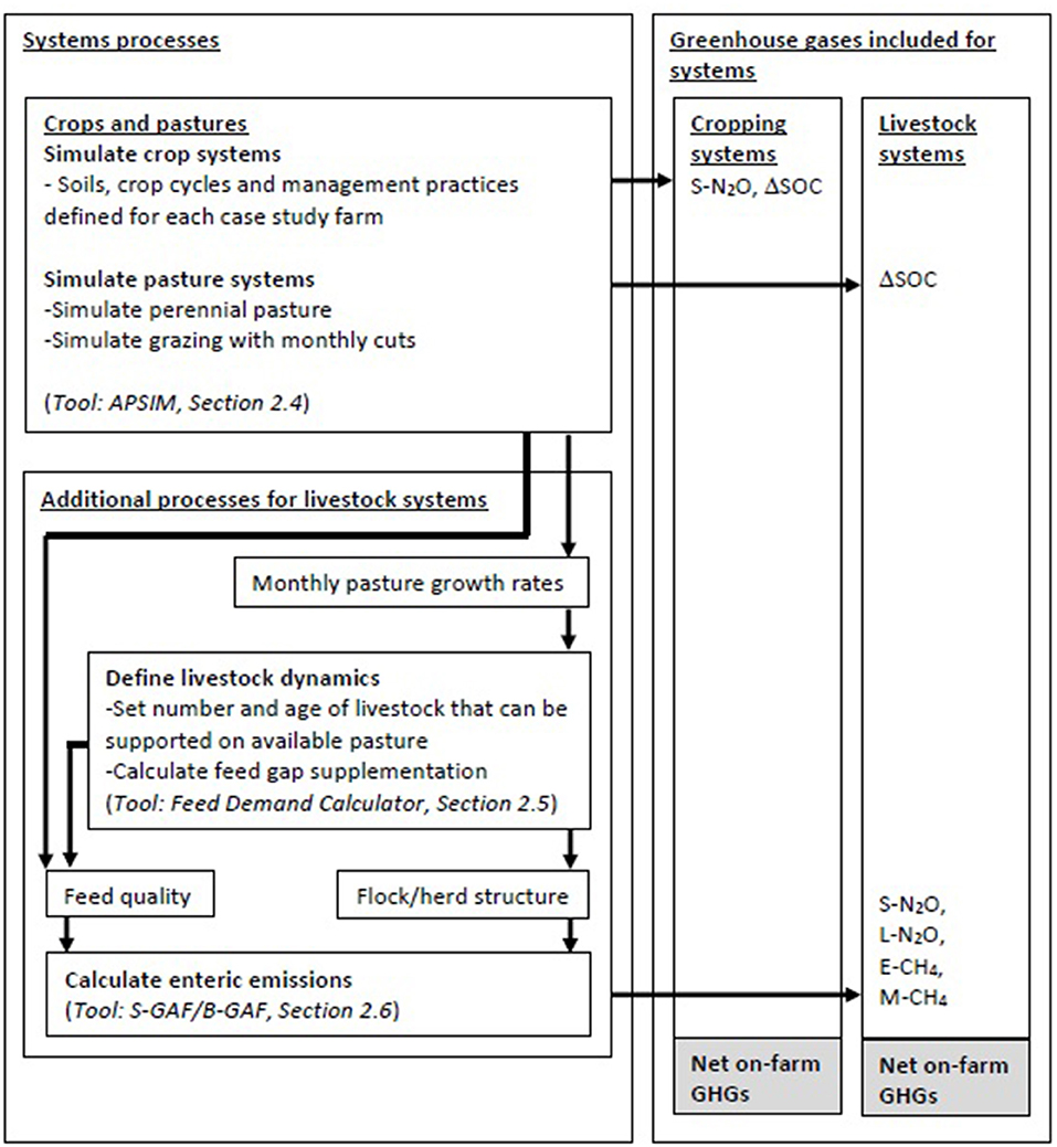
Figure 2. Overview of the approach used to integrate tools for simulating crops, pasture and livestock production and on-farm greenhouse gas (GHG) emissions for the case study farms. Greenhouse gas emissions included (1) N2O from the soil (S-N2O) and from urine and manure wastes from livestock (L-N2O), (2) CH4 from enteric sources (E-CH4) and from manure (M-CH4), and (3) the net change in atmospheric concentrations of CO2 derived from sequestration or decomposition of soil organic carbon (ΔSOC).
Livestock Systems
Livestock systems were simulated with an integrated approach utilizing several tools (Figure 2). Permanent pasture growth, and the ΔSOC and emissions of S-N2O associated with pasture production were simulated with the APSIM model (described in section Simulation of Crops and Pasture Systems With APSIM).
The monthly growth rate of pastures simulated with the APSIM model were used to estimate the annual feed base available to livestock at each farm. The flock or herd structure and stocking rates that could be supported by the simulated feed base were identified with the Meat and Livestock (MLA) Feed Demand Calculator (Bell et al., 2008; Moore et al., 2009). Purchases and sales of livestock required to maintain the flock or herd structure, and the amount of any supplements fed were estimated with the calculator (described in section Defining Livestock Dynamics With the Feed Demand Calculator).
The age and number of livestock and seasonal quality of feed established from using APSIM and the Feed Demand Calculator were inputs to the Sheep and Beef Greenhouse Gas Accounting Frameworks v6 (S-GAF and B-GAF, respectively; Browne et al., 2011). The S-GAF and B-GAF frameworks are described in section Calculating Emissions From Livestock With B-GAF and S-GAF. These tools provided estimates of the seasonal emissions of N2O from livestock urine and manure (L-N2O) and emissions of CH4 from enteric sources (E-CH4) and from manure (M-CH4). These emissions were combined with net balance of emissions from pasture production to estimate the total GHG profile of the livestock systems.
Simulation of Crops and Pasture Systems With APSIM
Crop and pasture plant production, ΔSOC storage and S-N2O emissions from crop and pasture production were simulated with the APSIM model configured with modules for soil nitrogen (APSIM-SoilN; Probert et al., 1998), soil water dynamics (APSIM-SoilWat; Probert et al., 1998), soil temperature (APSIM-SoilTemp2, following Campbell, 1985), residue (APSIM-SurfaceOM; Probert et al., 1998) and crop growth. All modules interact and processes are simulated with a daily time step, using historical daily climate data obtained from the SILO data base (Jeffrey et al., 2001) for weather stations close to the case study farms.
The crop rotations (Table 2), tillage, N fertilizer application, sowing and harvesting practices required for crop and pasture production at each farm (sections Crops and Management and Pastures and Management) were included in the simulations. All scenarios were simulated with the same initial soil properties. Each combination of location, soil, and crop or pasture was modeled over a 100 year period. Each combination was simulated for 10 different starting years (1906–1915) to prevent any potential cyclical patterns in the climate data interacting with the patterns in crop rotations.
Soil Processes
Soil carbon and nitrogen cycling in the APSIM-SoilN module were simulated by subdividing the soil C and N into inert, humic, fresh organic matter (i.e., roots) and microbial biomass pools that have constant C:N ratios (Probert et al., 1998). The C and N in the inert pool do not decompose, while the maximum potential decomposition rates for C from other pools vary. The humic pool decomposition rate is in the order of years while the microbial pool rate is in the order of days. The rate at which C flows between the pools is determined by fixed turnover rates for each pool. The amount of C decomposed from each pool is split between the receiving pool and evolved CO2, according to efficiency coefficients for each pool. The corresponding flows of N between pools are determined by the C:N ratio of the receiving pool; any shortfall or excess of N results in immobilization or mineralization, respectively, of mineral N. Nitrous oxide emission was calculated from the ratio of N2 to N2O emitted during denitrification; this fraction increased linearly from 0.00 to 1.18 as the percentage of water filled pore space increased from 21.3 to 100.0 (Thorburn et al., 2010).
In the APSIM-SoilWat module, the soil water characteristic in each soil layer was specified in terms of air dry, lower limit, drained upper limit and saturated volumetric water contents. Movement of soil water between the layers was simulated using a one dimensional “tipping” bucket process in which water moved between soil layers in the profile according to separate algorithms for saturated or unsaturated flow. Soil nitrate is assumed to be completely mixed with soil water, with leaching losses of nitrate occurring in proportion to its concentration in soil water.
The APSIM soil modules were set up with data for the specified soils (Table 1). These data included soil water characteristic information, hydraulic conductivity, SOC (including the allocation of SOC to microbial biomass, humic and inert SOC fractions), soil pH, runoff curve numbers and coefficients for first and second order evaporation. Soil profiles for each farm were configured with the number of layers defined for each soil (approximately seven layers), and processes associated with transformations of soil carbon, nitrogen and water were calculated for each layer. Parameter values for each soil are provided in the APSIM model soil database “APSoil” (Dalgliesh et al., 2012).
Residue Decomposition
Decomposition of crop and pasture residues were simulated with the APSIM-SurfaceOM module. Residues were transferred from the relevant plant model to SurfaceOM with a carbon fraction of 0.4 following detachment during the life of the plant or upon plant death. Crop and pasture residues were retained on the soil surface and decomposed in situ unless they were removed by burning. Simulated burning removed 70% of the residue dry matter, carbon and nitrogen from the field.
Crops and Management
Modules for wheat (Triticum spp.), barley (Hordeum vulgare), canola (Brassica napus), lupins (Lupins spp.), oats (Avena sativa), chickpea (Cicer arietinum), field pea (Pisum sativum), cotton (Gossypium spp.), and sorghum (Sorghum bicolor) crops were deployed with default parameters to simulate the different crop rotations (Table 2). The management practices used for crop establishment (e.g., plant density, sowing depth, and sowing window) and nitrogen fertilizer was provided by the farm owners and/or their advisors. Winter crops were sown between 25 April and 2 June if adequate rainfall was received within a specified period (e.g., 15 mm received in the preceding 10 days for wheat crops sown at Kellerberrin). Summer crops at Chinchilla were sown between 5 October and 15 January if soil water content exceeded 90% of drained upper limit in the surface 0.5 m of soil. If conditions for sowing were not satisfied, then crops were sown on the last day of the sowing window. N fertilizer management reflected that specified by farm owners and their advisors (Table 2). All simulated crops were rainfed with minimum tillage. Fallow periods were uncropped and kept free of weeds.
Pastures and Management
Permanent pastures of annual ryegrass (Lolium rigidum) or clover (Trifolium subterraneum ssp. Subterraneum “Dalkeith”) were simulated for the Kellerberrin and Southern Mallee case study farms in APSIM with the Ausfarm v1.4.13 Established Pasture module. For the Chinchilla case study farm, a Bambatsi (Panicum coloratum) and Bambatsi-medic (Medicago truncatula) pasture were simulated with the APSIM Bambatsi module and Ausfarm v1.4.13 Established Pasture module (medic). Average daily pasture growth rates for each month were calculated as the sum of net above-ground primary production for each month divided by the days per month, then averaged over the simulation period. Pasture biomass in excess of 50 mm height at Kellerberrin and Southern Mallee, or 3,500 kg biomass ha−1 at Chinchilla, was cut and removed at monthly intervals to simulate removal of biomass by grazing. This pasture management was adopted in order to maintain a long-term average conservative pasture utilization rate of 30% (described in section Defining Livestock Dynamics With the Feed Demand Calculator). The remaining pasture could regrow in simulations. The N recycled in livestock urine and manure was simulated by applying manure each month at rates proportional to the number of livestock (Barker et al., 2002). The effect of trampling and selective grazing was not included in simulated pasture management. All pastures were simulated under rainfed conditions. Fertilizer was applied to pastures in the Livestockgrass scenario at the rate of 12.5–50 kg urea-N ha−1 yr−1 to maintain productivity over the 100 year simulation period, consistent with recommended practice (Eckard, 2010); pastures in the Livestocklegume scenario included legumes and were not fertilized with N.
Feed quality was defined in terms of values simulated with APSIM for dry matter digestibility (DMD), and with values obtained from the literature for crude protein (CP) and metabolizable energy (ME). A range of quality parameters was used for feed based on pastures to reflect seasonal changes in pasture quality during the year. These values were set as follows: annual ryegrass [5–11% CP, 45–70% DMD, 7–12% MJ ME (kg DM)−1], clover [7–17% CP, 62–72% DMD, 7–11% MJ ME (kg DM)−1], Bambatsi [5–16% CP, 47–60% DMD, 7–9% MJ ME (kg DM)−1], and lupin grain fed as supplement [30% CP, 86% DMD, 13 MJ ME (kg DM)−1] (Courtney, 2002; Lloyd, 2007).
Defining Livestock Dynamics With the Feed Demand Calculator
Simulated long-term pasture growth rates, available supplements and the ME of all feed sources were input to the Feed Demand Calculator (Bell et al., 2008; Moore et al., 2009) to determine the amount and timing of feed available to support livestock numbers throughout the year at each case study farm. Pasture growth at the locations is strongly seasonal in response to rainfall (Figure 1) and requires careful stocking to avoid soil degradation when ground cover is low. Flock or herd structures that were representative of local practice were defined for each case study farm and designed so that animal demand was lowest during periods of low pasture growth and vice versa (described in succeeding paragraphs in this section). The long-term average sustainable number of livestock for each farm was determined by the amount of feed available from the different pasture scenarios to satisfy livestock demand for energy at a pasture utilization rate of 30% of net above-ground primary pasture growth per year [Hunt, 2008; MLA (Meat and Livestock Association) and CSIRO (Commonwealth Scientific and Industrial Research Organisation), 2013]. The stocking rates therefore differed between livestock scenarios based on differing pasture quantity and quality, and were maintained in each year throughout the simulation period at each farm. Thus, while the pasture utilization rate was more conservative than rates that could sometimes occur in response to tactical grazing management [MLA (Meat and Livestock Association) and CSIRO (Commonwealth Scientific and Industrial Research Organisation), 2013], it was necessary to support long-term stocking rates that were sustainable given static livestock management. Livestock demand accounted for energy requirements for maintenance, lactation and growth and was predicated on typical annual cycles of reproduction and growth. Feed requirements and stocking rates were compared for different classes of animals by expressing them in Dry Sheep Equivalents (DSE), i.e., the amount of feed required by a 2 year-old, 45 kg sheep wether or non-pregnant and non-lactating ewe (McLaren, 1997).
Livestock at the Kellerberrin and Southern Mallee case study farms consisted of a breeding flock of Merino sheep with rams included in the ratio of one ram per 100 ewes. Ewes were joined from 1 November to 15 February each year with a weaning rate of 0.8 lambs per ewe. Annual livestock sales occurred in November when all lambs were at least 4 months old. Ewe lambs replaced 20% of the breeding flock each year. The breeding ewes that were replaced, and all remaining lambs, were then sold. The diet of sheep at the Kellerberrin and Southern Mallee case study farms was supplemented from February to May with lupin grain at the rate of 46 kg DSE−1 yr−1 (Finlayson et al., 2012). Supplements were assumed to be 100 % consumed by the sheep without wastage. This flock structure and management was used in both livestock scenarios.
Livestock at the Chinchilla case study farm consisted of a trading herd of Bos taurus x Bos indicus steers. Ten month-old steers weighing 200 kg head−1 (equivalent to 6.5 DSE each; McLaren, 1997) were purchased in cohorts on the first of January, April and October, and sold 15 months later at 400 kg head−1. The diet of the steers consisted of pastures in the Livestockgrass and Livestocklegume scenarios without additional supplementation. This structure and management of the trading herds was used in both livestock scenarios.
Calculating Emissions From Livestock With B-GAF and S-GAF
Greenhouse gas emissions from livestock manure, urine and E-CH4 were calculated using the S-GAF and B-GAF emissions calculators (Figure 2). The calculators use Australian National Greenhouse Gas Inventory methods prescribed by the [DCCEE (Department of Climate Change and Energy Efficiency), 2012] to compute the whole-farm emissions in terms of CO2 equivalents (CO2e) from animal production (number, class of livestock, weight, and live weight gain), N fertilizer inputs and pasture quality (dry matter availability, crude protein, and dry matter digestibility). Emissions from livestock are dominated by E-CH4, which is closely related to dry matter intake [DEE (Department of the Environment and Energy), 2017]. Australian livestock production occurs in many cases in semi-arid and subtropical climatic conditions. Consequently, typical animal performance tends to vary from those used to define default animal emissions (e.g., many European countries), and so country-specific emissions factors have been used in the calculators to better represent stock weight for age, weight gain, feed quality, and manure management [DEE (Department of the Environment and Energy), 2017].
Modeled Scenario Evaluation
Simulation tools have been validated in other studies for (1) APSIM crop and pasture systems (Carberry et al., 2009; Pembleton et al., 2013; Meier et al., 2017) including simulation of SOC and N2O emissions in similar soils and climates (Luo et al., 2011; Liu et al., 2014; Mielenz et al., 2016; O'Leary et al., 2016); and peer-reviewed application of (2) the Feed Demand Calculator (Bell et al., 2008; Moore et al., 2009); and (3) S-GAF and B-GAF (Browne et al., 2011; Harrison et al., 2014a,b). For simulation of ΔSOC with APSIM described in (1), close correspondence with measured values was obtained in these references for experimental periods of up to 44 years with RMSE values of 1 to 11 Mg SOC ha−1 (0.0–0.3 m). Close correspondence of simulated and measured seasonal N2O emissions was also demonstrated with RMSE values of 0.052–0.441 kg N ha−1 (Mielenz et al., 2016) and with simulated emissions within ±10% of measured values (Meier et al., 2017). While these publications demonstrate the credible simulation capacity of these tools, the simulations are not for the precise locations of the case study farms and do not use the model set ups described in these publications. Further, the simulation of ΔSOC could not be tested against on-farm measurements because the initial SOC used was obtained from measured values on nearby soils (Table 1) and ΔSOC was not measured during the 100 year simulation period. For this reason, simulated long-term ΔSOC for the farms is presented in supplementary material to demonstrate the credible response of simulated SOC within the scenarios. The evaluation of simulation results against measured values was therefore made against crop yield, pasture net above-ground primary production and stocking rate results reported from the farms and from nearby locations to assess the accuracy of the simulated plant production.
Calculations for GWP
Emissions From Soil
On-farm greenhouse gas emissions from the soil (S-N2O and ΔSOC) were simulated with APSIM (section Simulation of Crops and Pasture Systems With APSIM). The emissions were converted to the common units of carbon dioxide equivalents (CO2e) using the 100 year conversion factor with climate-carbon feedback of 298 for S-N2O (IPCC, 2013). The change in SOC stocks (0.0–0.3 m) was multiplied by 3.67 to convert carbon to the equivalent mass of CO2e.
Emissions From Livestock
Whole-farm emissions of S-N2O, L-N2O from livestock manure and urine, and E-CH4, were each calculated with the S-GAF and B-GAF calculators in terms of CO2e (section Calculating Emissions From Livestock With B-GAF and S-GAF). The emissions were converted to the common units of carbon dioxide equivalents (CO2e) using the 100 year conversion factor with climate-carbon feedback of 298 for N2O and 34 for CH4 (IPCC, 2013). The emissions were converted to values per unit area (Mg CO2e ha−1) to facilitate comparison of emissions between cropping and livestock systems and between farms.
Net GWP
The net on-farm GWP of scenarios for each of the scenarios was calculated as the sum in CO2e ha−1 of GHG emissions (S-N2O, L-N2O, E-CH4, and ΔSOC) simulated for each site. The GWPs calculated for scenarios were restricted to on-farm emissions from crop and livestock systems and hence emissions associated with off-farm activities (e.g., manufacture and transport of N fertilizer) were excluded from the analysis. Tukey's Honestly Significant Difference test (Yandell, 1997) was used to identify significant differences (p < 0.05) between the scenarios for ΔSOC, N2O, CH4, and GWP in the RStudio statistical package (v0.99.465).
Emissions Intensities
The emissions intensity of the different scenarios was calculated as the annual per hectare emissions in CO2e per kilogram of protein in harvested grain for cropping scenarios or per kilogram of edible protein in dressed carcasses sold for livestock scenarios. The percentage protein content used in calculations for harvested grain was 10.6 (sorghum), 11.0 (wheat), 12.5 (barley), 36.2 (lupin), 22.5 (canola), 20.5 (chickpea), 23.0 (field pea), and 9.4 (maize) [Province of Manitoba, 2004; Pulse Australia, 2018; USDA (United States Department of Agriculture), 2018]. Meat protein was calculated assuming that dressed carcass weight was 60% of live weight for cattle and 50% for sheep (Raines, 1999), with protein in the carcass of 17.5% for beef [USDA (United States Department of Agriculture), 2018] and 15.6% for lamb (Hankins, 1947). The protein in by-products such as stover in the cropping scenarios or in wool and hides in the animal scenarios was not included in the calculation of emissions intensities.
Results
Validity Tests for Model Outputs
Crop Yields
The simulated crop yields at each case study farm were compared with point estimates of typical yields provided by the farm owners (Figures 3A–C). There was a greater range of simulated yields compared to point estimates because these yields were simulated over 100 yr of climate data in each location and thus reflected a broader range of climatic conditions (Figure 1). Nevertheless, farm yields typically occurred within the second and third quartiles of simulated yields; thus, simulated yields were considered representative for the locations.
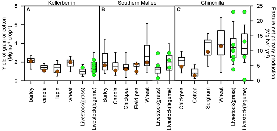
Figure 3. Simulated (box and whiskers plots) and reference crop (brown symbols) and pasture yields (green symbols) at the (A) Kellerberrin, (B) Southern Mallee, and (C) Chinchilla case study farms. Permanent pastures consist of grass receiving 12.5–50 kg N fertilizer ha−1 yr−1 (Livestockgrass scenario) and a legume pasture that was not fertilized with N (Livestocklegume scenario). Reference yields for crops represented typical crop yields at the farm as described by the farm owners. Reference yields for pastures were sourced from the literature as follows: for Kellerberrin, Puckridge and French (1983), Bolger and Turner (1999), Latta et al. (2001), Fillery and Poulter (2006), Brennan et al. (2013); for Southern Mallee, Puckridge and French (1983), Descheemaeker et al. (2014); for Chinchilla, Lloyd (1981, 2007), Lloyd et al. (1983), Cook et al. (2005). “Whiskers” in the box and whisker plots are provided for 5 and 95% of simulated values.
Pasture Production
The long-term simulated net above-ground pasture primary production at the case study farms was in close agreement with values provided in the literature (Figures 3A–C). The main predictors of pasture regrowth rates are rainfall, minimum temperature and maximum temperature [MLA (Meat and Livestock Association) and CSIRO (Commonwealth Scientific and Industrial Research Organisation), 2013], and so the simulated pasture growth rates for the Livestockgrass and Livestocklegume scenarios in combination were also compared with values from the literature (Figures 4A–C). The median value of simulated pasture growth rates was consistent across all sites with reference values reported by Meat and Livestock Australia [MLA (Meat and Livestock Association) and CSIRO (Commonwealth Scientific and Industrial Research Organisation), 2013; MLA (Meat and Livestock Association), 2019] and the Future Farm Industries Cooperative Research Centre [FFICRC (Future Farm Industries Cooperative Research Centre), 2013]. These reference values were reported for sites located between 80 and 200 km from the case study farms: at Northam for the Kellerberrin farm, at Boort and Balmoral for the Southern Mallee farm, and at Roma for the Chinchilla farm. There was also potential at Chinchilla for high pasture growth rates of two to three times the median growth rate to occur, but this high production potential and high variability in growth was consistent with field experimental values reported by Lloyd (1974).
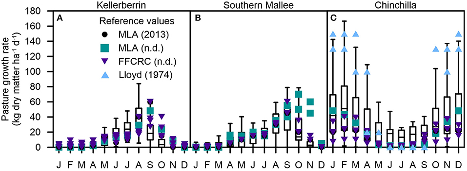
Figure 4. Simulated (box and whisker plots) and reference values (symbols) for pasture growth rates at the (A) Kellerberrin, (B) Southern Mallee, and (C) Chinchilla case study farms. Simulated values include those from both the Livestockgrass (grass pasture receiving 12.5–50 kg N fertilizer ha−1 yr−1) and Livestocklegume (legume pasture) scenarios because pastures are subjected to the same temperatures and rainfall influencing pasture growth. “Whiskers” in the box and whisker plots are provided for 1.5 × the interquartile range.
Livestock Management
Stocking rates in the livestock systems ranged from 1.7 to 3.5 DSE ha−1 at Kellerberrin, 2.0 to 4.4 DSE ha−1 at Southern Mallee, and 6.3 to 8.5 DSE ha−1 at Chinchilla, with ranges reflecting changes due to births, purchases and sales (Figures 5A–C). These stocking rates were generally consistent with or lower than values reported in the literature (Figures 5A–C). The lower rates occurred because a relatively conservative pasture utilization objective of 30% was adopted the simulation period, to allow for seasonal variability in pasture production during the 100 yr simulation period. It is possible that short term pasture utilization rates of up to 60% can be achieved depending upon type of livestock, opportunistic management and environmental conditions [MLA (Meat and Livestock Association), 2019], whereas the average long-term pasture utilization rate simulated at all locations was 26–32% of the net above-ground primary production.
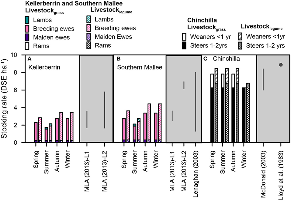
Figure 5. Simulated stocking rates (white panels) and point values or range of values for reference stocking rates (gray panels) for the (A) Kellerberrin, (B) Southern mallee, and (C) Chinchilla case study farms. Note that rams at Kellerberrin and Southern Mallee represent ≤0.02 DSE ha−1 of the overall stocking rate at these locations and are not visible in the bars. Permanent pastures consist of grass receiving 12.5–50 kg N fertilizer ha−1 yr−1 (Livestockgrass scenario; solid bars) and a legume pasture that was not fertilized with N (Livestocklegume scenario; hatched bars).
Long-Term Average GHG Profiles for Scenarios
ΔSOC
SOC fluctuated at all locations during the simulation period and approached equilibrium values by the end of the simulation period (Figure 6). Greater variability occurred within the cropping compared to livestock scenarios due to cyclical differences in inputs to SOC throughout the year from cropped phases followed by weed-free fallows (especially in cropping scenarios at Kellerberrin and Southern Mallee where Cropburn and Cropstubble had weed-free summer fallows but low summer rainfall also limited inputs of SOC during fallows under the Cropintensity scenario). Changes in SOC in some scenarios over the simulation period indicated that SOC at the start of the simulations was not at equilibrium by reference to the different scenario managements; this was expected because all simulations started with the same initial starting SOC but had differences in SOC inputs (described below). The relative change in SOC between scenarios elicited from this starting point was important for comparing scenarios in this study.
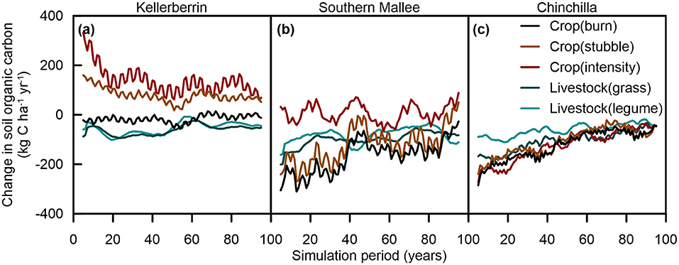
Figure 6. Average change in soil organic carbon (ΔSOC) for the cropping scenarios, Cropburn (burnt stubble), Cropstubble (retained stubble), and Cropintensity (increased cropping intensity), and livestock scenarios, Livestockgrass (permanent grass pasture) and Livestocklegume (permanent improved pasture), at the (a) Kellerberrin, (b) Southern Mallee, and (c) Chinchilla case study farms.
Changes in SOC (expressed as CO2e, Figures 7A–C) varied between scenarios and farms due to the interaction between farm-specific differences in rainfall patterns, soil properties and initial SOC with differences between scenarios in organic matter inputs. Depending upon the location, the amount of organic matter inputs from crop residues and roots at harvest in the cropping scenarios were roughly 2, 4–5, and 5–6 Mg organic matter ha−1 yr−1 in the Cropburn, Cropstubble, and Cropintensity scenarios, respectively (data not shown). The amount of organic matter inputs from residues and roots to the livestock scenarios was roughly 2–3 and 3–4 Mg organic matter ha−1 yr−1 from the Livestockgrass and Livestocklegume scenarios, respectively. Consequently, there was potential for greater increase or lower decrease in SOC under the cropping scenarios than the livestock scenarios. However, the pattern of organic matter additions differed between the systems and was important for ΔSOC: most organic matter additions occurred at harvest in the cropping scenarios but occurred throughout the year in the livestock pasture scenarios. The interaction of the rate of organic matter inputs with seasonal rainfall and soil moisture capacity was also important for the rate of decomposition of residues: for example, deposition of cropping residues at harvest at Kellerberrin and Southern Mallee were typically followed by dry summers with low potential for crop residue break down. In addition to these interactions between farm-specific climates and the amount and timing of organic matter inputs, the capacity for an absolute increase in SOC at the locations was influenced by initial SOC content. Therefore, there was an absolute increase in SOC in response to cropping scenarios at Kellerberrin from a low initial SOC of 0.5 to 0.6%C (Table 1; Figure 7A) but only relative changes in SOC resulted at other locations with higher initial SOC (≥1.1%; Figures 7B,C).
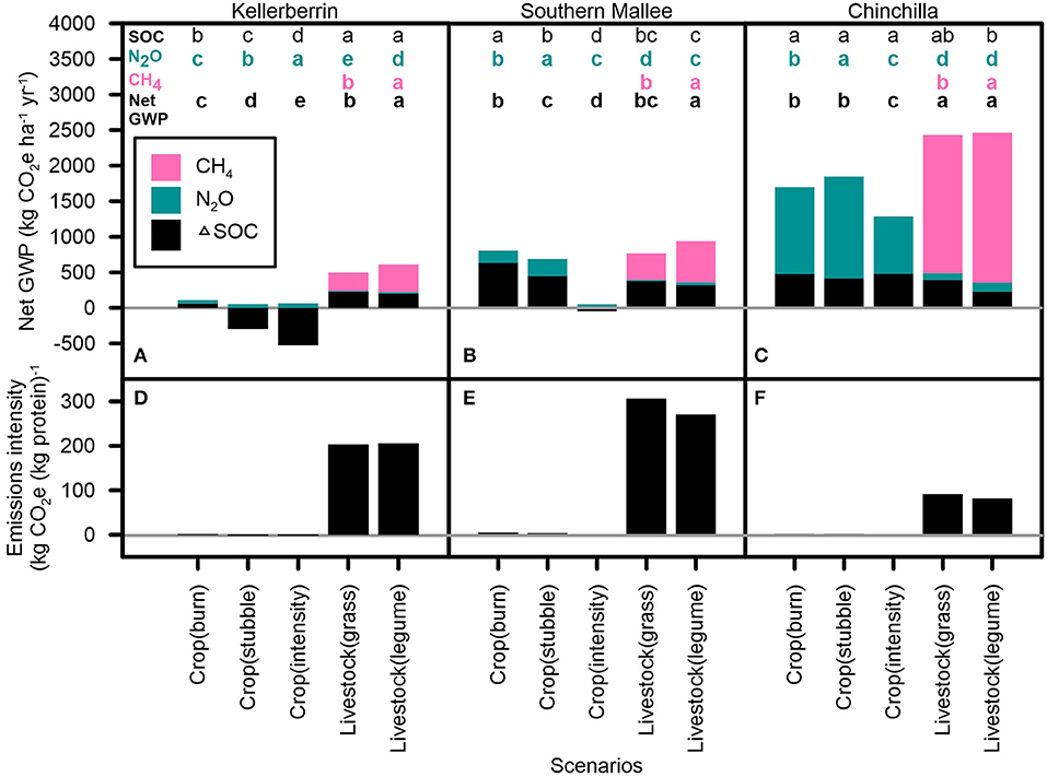
Figure 7. Average net global warming potential (GWP) (A–C) and emissions intensities (D–F) for the cropping scenarios, Cropburn (burnt stubble), Cropstubble (retained stubble), and Cropintensity (increased cropping intensity), and livestock scenarios, Livestockgrass (permanent grass pasture) and Livestocklegume (permanent improved pasture), at the Kellerberrin, Southern Mallee, and Chinchilla case study farms. In (A–C), net GWP is the sum of average annual on-farm emissions of (1) CO2 associated with the change in soil organic carbon (ΔSOC), (2) N2O from the soil, manure and urine, and (3) CH4 from enteric fermentation and from manure. Scenarios that differ by more than the honestly significant difference value in these individual emissions or net GWP have a different letter shown at the top of the panel. Negative values for net GWP represent abatement from the scenarios. Emissions represent the average of values from the 100 yr simulation period. In (D–F), emissions intensities are calculated for cropping in terms of harvested grain protein and for livestock scenarios in terms of the protein content of dressed animal carcasses sold. Long-term average emissions intensities for cropping systems were very small [−1.2 to 4.3 kg CO2e (kg protein)−1] and may be difficult to distinguish for some farm-scenario combinations.
These interactions led to differences in the ΔSOC between the farms. For example, the long-term average annual GHG emissions of CO2 from ΔSOC were significantly lower (i.e., less SOC was decomposed) in the Livestocklegume scenario than the Cropburn scenario at Southern Mallee and in the Livestocklegume than all crop scenarios at Chinchilla, because of the larger organic matter inputs in Livestocklegume. However, this situation was reversed at the Kellerberrin farm, where well-drained soils received least summer rainfall and cropping residues deposited at harvest decomposed more slowly than for the Livestocklegume residues deposited throughout the year.
N2O
Nitrous oxide emissions were a substantial proportion of the GHG profile for cropping scenarios at both the Chinchilla and Southern Mallee farms. For the cropping scenarios at Chinchilla, the long-term average emissions of N2O were up to 1.4 Mg CO2e ha−1 yr−1. For all other scenarios and locations apart from the cropping scenarios at Chinchilla, emissions of N2O were a relatively small proportion of the emissions profile and were ≤ 0.2 Mg CO2e ha−1 yr−1.
CH4
For all farms, emissions of CH4 were significantly greater from the Livestocklegume than Livestockgrass scenario (Figures 7A–C), consistent with the higher stocking rates maintained in the Livestocklegume scenario (Figures 5A–C). As stated in section Cropping Systems, emissions of CH4 were assumed to be minor for the cropping systems and were not simulated for those scenarios.
Net GWP
Although the Livestocklegume scenario had lower emissions from decomposition of SOC compared to Cropburn or Cropintensity at some sites, the net GWP from all emissions was consistently lowest from the Cropintensity scenario at all farms (Figures 7A–C). At the Southern Mallee and Chinchilla farms, the emissions of N2O from the Cropburn and Cropstubble scenarios were similar to the emissions of CH4 from the Livestockgrass and Livestocklegume scenarios. This led to similar net GWP between the Cropburn, Cropstubble, Livestockgrass, and Livestocklegume scenarios for these farms. At the Kellerberrin farm, both the Cropstubble and Cropintensity scenarios provided abatement (rather than merely lowering net GWP) compared to net emissions from the Livestockgrass and Livestocklegume scenarios due to significant SOC sequestration at this site.
Emissions Intensities
Emissions intensities for the livestock scenarios ranged from 81 to 306 kg CO2e (kg dressed carcass protein)−1) (Figures 7D–F) and were markedly lower at Chinchilla [average 91 and 81 kg CO2e (kg live weight)−1 in Livestockgrass and Livestocklegume scenarios] than for other locations. These lower emissions intensities for livestock systems also declined between the Livestockgrass and Livestocklegume scenarios at Chinchilla and Southern Mallee as stocking rates increased in response to improved pasture, but this change was small [10–36 kg CO2e (kg dressed carcass protein)−1] compared to the variation in emissions intensities caused by location. The average emissions intensities for cropping scenarios were relatively small by comparison to the livestock system scenarios and ranged from −0.9 to 4.3 kg CO2e (kg grain protein)−1.
Discussion
This study sought to compare long-term net GHG abatement of stocked permanent pastures relative to cropping systems. We found that, for our case study farms, net emissions from stocked permanent pastures were not always less than those from cropping systems. This was because enteric CH4 emissions from livestock were not consistently offset by increased SOC under permanent pastures relative to the cropped systems (Figure 6). Thus, the key messages from this paper is that it is crucial to consider all GHG emissions when evaluating the abatement potential of different farming systems and practices, and that these practices need to be tailored to the climate, crops, soils, and management at locations.
While SOC sequestration from agricultural practices can contribute to climate change mitigation (e.g., from pastures: Post and Kwon, 2000; Guo and Gifford, 2002; Sanderman et al., 2010; Hoyle et al., 2011; Kragt et al., 2012), the impact of changes in SOC are often considered in isolation from emissions corresponding to the land use change, e.g., from emissions from livestock feeding on pastures that have been converted from cropped land (e.g., Guo and Gifford). For the case study farms used in this study, the annual emissions of N2O from soils in cropping scenarios and of enteric CH4 from livestock scenarios were a substantial portion of net GWP profiles of the case studies (Figures 7A–C). For example, the long-term average ΔSOC was not significantly different for some cropping and livestock scenarios at the Chinchilla and Southern Mallee case studies (Figures 7A–C), and so neither scenario would provide an advantage for GHG emissions reductions unless either the N2O could be reduced in the cropping scenario or CH4 emissions in the livestock scenario. This study therefore also highlights the importance of evaluating different practices based on emissions that are ongoing (N2O and CH4 emissions) in addition to considering the impact of practices on ΔSOC, since the former can only be reduced rather than mitigated. This consideration becomes increasingly important as emissions from ΔSOC approach equilibrium values in response to changes in practices.
In Australia, there are government policies that encourage the agricultural sector to contribute to national GHG emissions reductions targets through the mechanism known as the Emissions Reduction Fund (Clean Energy Regulator, 2015). In this policy, participants can be remunerated for GHG emissions reductions that they achieve using prescribed methodologies [DEE (Department of the Environment and Energy), 2019]. One of these methods is the conversion of crop land to permanent pasture (Australian Government, 2015). However, in this study we find that permanent pastures do not necessarily provide abatement where the pastures are stocked and emissions from livestock are considered, and thus achieving national abatement objectives could be compromised by adopting this practice. There are clearly lessons from this experience in Australia for other countries considering GHG abatement policies for the land sector.
Building SOC in agricultural soils has been identified as a substantial opportunity for mitigating GHG emissions (e.g., the 4 per 1,000 Initiative; http://4p1000.org/understand), and the establishment of permanent pastures or pasture phases identified as a practice for storing SOC in cropping systems (e.g., Sanderman et al., 2010; Luo et al., 2011; Rabbi et al., 2014; Murphy, 2015). However, in the case studies considered here, we found that permanent pastures supporting livestock did not necessarily sequester more SOC or provide more GHG abatement than cropping systems. While our findings contrast with other research, the results for our case studies can be attributed to the greater inputs to SOC under the cropping than livestock systems scenarios (section ΔSOC). A key influence upon C inputs to soils for the Kellerberrin and Southern Mallee case studies is that low summer rainfall limits pasture growth in the livestock scenarios to a similar period to that in which crops are grown in the cropping scenarios. At the same time, the pastures in the livestock scenarios received little or no fertilizer, further limiting pasture growth and the inputs of carbon to soils in the livestock scenarios compared to inputs to SOC from crops in the cropping scenarios. While it is possible to simulate pasture systems with higher fertilizer inputs and potentially increased biomass and SOC inputs, in practice fertilizer applications to pastures in these regions often unprofitable (because low rainfall limits pasture growth potential), so the actual SOC sequestration under pastures will commonly be lower than the technical sequestration potential. The potential for climate to limit the accumulation of SOC has been recognized in previous studies. Liu D. L. et al. (2016) predicted this result at sites with low annual rainfall (443 mm yr−1), while Lawes and Robertson (2012) found no significant difference in SOC under annual pastures adjacent to perennial pastures of 10 years age (a comparison analogous to crop and permanent pasture systems) at sites receiving rainfall of 400–500 mm yr−1. The climatic conditions in these studies are similar to the conditions described for our case study sites (Table 1; Figure 1) and are common in crop and livestock production under areas in much of Australia. Thus, while improving the quality of pastures (e.g., the change from scenario Livestockgrass to Livestocklegume) results in substantial increases in both dry matter and SOC in other locations, such as in Brazil where annual rainfall averages 1,300 mm or more (Climate-Data.Org, 2018) and potential growth rates are high (e.g., de Oliveira Silva et al., 2015, 2016; Dick et al., 2015; Mazzetto et al., 2015), this practice is less effective under the lower, seasonal rainfall experienced at the Kellerberrin and Southern Mallee case study sites.
The soil-based emissions approach adopted in this study was limited by not including sources of GHGs from fuel use or off-site sources such as the emissions embodied in production and transport of inputs like fertilizer. These emissions have implications for the Cropintensity and Livestocklegume scenarios for example, in which N supplied by legumes substitutes for N inputs otherwise provided by fertilizer and reduces this portion of off-site emissions associated with production from these scenarios. Assessment of the emissions from all sources, while complex, is important to ensure that both field-scale and absolute abatement is achieved when evaluating the abatement potential of different practices (e.g., de Boer et al., 2011). However, the potential for pastures to provide abatement has often been identified based solely on their capacity to sequester SOC (e.g., Guo and Gifford, 2002). In the parallel approach adopted for this study, we have similarly evaluated only the soil-based emissions from cropping systems and have added emissions from livestock to the ΔSOC from pastures. While this approach falls short of a life cycle analysis (LCA) approach in which cradle-to-grave emissions are evaluated, it holds merit in that the emissions reported may provide less uncertainty than the additional GHGs that could also be reported. For example, emissions associated with ΔSOC, N2O and CH4 have been well-tested in the APSIM, S-GAF and B-GAF models (see section Modeled Scenario Evaluation). The additional GHGs associated with on-farm practices of fuel, lime and pesticide use, and pre and post farm emissions are highly management- and site-specific, so the less-subjective emissions presented in this study are useful here for comparing practices.
An additional limitation of our study may be that the contribution of livestock to emissions from pastures has been overstated due to the livestock management adopted. Farm livestock management was based on typical management practices that currently occur for livestock in the case study regions (Bell et al., 2008; Browne et al., 2011), which may not represent best management practices for GHG mitigation. Many practices have been identified that can reduce GHG emissions from crop and livestock systems, such as improved or alternative management of nutrients in cropping systems, and diet manipulation for ruminant livestock systems (e.g., Eckard et al., 2010; Liu C. et al., 2016; Smith et al., 2017). For the Southern Mallee and Chinchilla farms, where the net GWPs of the Cropburn and Cropstubble scenarios was not significantly different from the Livestockgrass and Livestocklegume scenarios (Figure 7), the adoption of these practices might alter our results and lead to a lower net GWP from the livestock scenarios than some of the cropping systems. The use of alternative practices is frequently limited by economics in marginal production areas such as Kellerberrin; nevertheless, adoption of these better practices could reduce the net GWP of any of the crop or livestock scenarios and requires further investigation for the diverse biophysical conditions occurring on the case study farms. Similarly, opportunistic management in both the crop and livestock scenarios could reduce the GWP of these scenarios by increasing crop and pasture growth in years of above-average rainfall and thus increase inputs to SOC. For example, an increase in stocking rate for the livestock scenarios has in some studies led to an increase in SOC (e.g., Sanderman et al., 2010) and thus could have reduced the net GWP of livestock scenarios, if these gains in ΔSOC exceeded additional emissions of CH4 arising from the higher number of stock. Stocking rates were increased from the Livestockgrass to Livestocklegume scenario in response to better pasture quality and quantity, but higher stocking rates within a scenario were not evaluated in this study because the simulated rates were sustainable for long-term simulations given low dry season pasture growth rates (section Defining Livestock Dynamics With the Feed Demand Calculator; Figure 4). However, there is potential for opportunistic increases in stocking rate (e.g., with a trading herd or flock) for seasons of better pasture growth as noted in section Defining Livestock Dynamics With the Feed Demand Calculator, and this possibility also warrants further investigation.
Other assumptions in the study may have contributed to relatively greater emissions intensity profiles for the livestock scenarios. Firstly, we assumed that the improved diet provided to livestock from the Livestocklegume scenario was used to support a greater stocking rate on the farm (Figure 5). Improvements in dietary quality are often used to demonstrate the more rapid attainment of target weights and consequent reduction in emission intensities for individual stock (e.g., Eckard et al., 2010). However, the profitability of livestock enterprises is linked to stocking rates (e.g., Amidy et al., 2017), and so in this study the increased pasture quality achieved under the Livestocklegume scenario was used to increase stock numbers on the farm, with the result that there was little difference between emissions and emission intensities between the Livestockgrass and Livestocklegume scenarios (Figure 6). Secondly, we have assumed crop or livestock-only farms in order to evaluate the practice of using pastures to generate net GHG abatement compared to cropping systems. However, many farms in southern Australia (e.g., where Southern Mallee and Kellerberrin are located) operate as mixed crop-livestock systems (Bell et al., 2008; Bell and Moore, 2012), while livestock-only farms are atypical for this area. For livestock, this may mean that some supplements are replaced with lower quality crop residues, potentially increasing emissions of E-CH4 (Eckard et al., 2010). For cropping systems, soil C and N cycling will be altered by decreasing inputs of stover and increasing inputs of manure and urine to SOC. These differences in management for a mixed farm are outside the scope of this study but could alter the emissions intensity from production of both crop and livestock products.
The results obtained from this study were site-specific and accounted for biophysical farm configurations and local farming practices such as crop selection, fertilizer use and rotations. As such the study does not provide the broader coverage that a global study could deliver; however, it highlighted important site-specific characteristics for GHG abatement, especially the interaction between soil properties, climate, plant production and GHG emissions. For example, differences between the case studies at Chinchilla and the other locations in soil properties and the amount and seasonality of rainfall contributed to marked differences in N2O emissions and emissions intensities for this farm (Table 1; Figures 1, 7). Larger N2O emissions occurred from cropping scenarios at Chinchilla than other farms (Figure 7) because this site had more slowly drained soils, received higher rainfall, and had a rainy season in summer, so there was greater potential for nitrification and denitrification to occur from soil that was both warm and wet. The significant reductions in N2O emissions at Chinchilla from the Cropintensity scenario therefore occurred because the additional crops simulated for this scenario used some stored soil water and reduced the potential for N2O emissions to occur.
In a second example from our results that demonstrates site-specific characteristics for GHG abatement, the emissions intensities from livestock systems were 125–201 kg CO2e (kg dressed carcass protein)−1 lower for Chinchilla than the other locations. Despite the higher overall net GWP of livestock systems from this farm compared to the other sites, the livestock emissions intensities were lower for two reasons. Firstly, higher rainfall at Chinchilla enabled greater annual pasture growth and hence of livestock weight gain and sales per year. Secondly, the livestock at Chinchilla were managed as a trading herd and so the emissions from all animals could be attributed to all the animals when sold. By comparison, breeding flocks were retained at Kellerberrin and Southern Mallee so annual emissions from all stock could only be attributed to a smaller number of stock sold (lambs and cull ewes). Understanding how different locations and systems provide GHG abatement is important for delivering abatement at the broader national and global scale. Accordingly, substantial caution should be applied when identifying agricultural management practices expected to deliver broad scale abatement, since interactions between temporal patterns of rainfall, total rainfall, temperature, drainage and management properties can lead to variable outcomes at different locations.
Conclusions
Permanent pastures stocked with ruminants may offer no GHG abatement advantage over cropping systems for a diverse range of Australian agricultural environments. GHG abatement practices identified for broad abatement potential in both crop and livestock systems should be selected with caution because differences in the amount and seasonality of rainfall and soil characteristics can shift the net GWP of locations from net abatement to net emissions, and assumptions about the GHG outcomes of different practices or farming systems (e.g., crops vs. livestock) maybe incorrect. Additionally, such practices should not be evaluated based on the response of a single GHG abatement process, such as potential SOC sequestration, but should only be recommended after considering the net GWP from all GHGs involved. It is also important to consider the “feedbacks” that happens when farm management is changed: for example, improving the quality and quantity of pasture fodder (as in moving from the Livestockgrass to Livestocklegume scenario) may not reduce whole farm livestock GHG emissions where the stocking rate is increased to exploit the better forage supply.
Data Availability Statement
The datasets generated for this study are available on request to the corresponding author.
Author Contributions
EM performed the methods and wrote the manuscript with input from PT, LB, MH, and JB. PT conceived the idea that GHG abatement from pastures may be negated by GHG emissions from livestock utilizing the pastures. LB and MH provided advice on appropriate livestock and pasture systems for locations and for the set-up of APSIM and GHG calculators for livestock scenarios. EM set up cropping scenarios with input from JB.
Funding
This work was supported by the CSIRO, the Australian Government and the Grains Research and Development Corporation (grant number CSE00057).
Conflict of Interest
The authors declare that the research was conducted in the absence of any commercial or financial relationships that could be construed as a potential conflict of interest.
Acknowledgments
We acknowledge the contributions of Scott Dixon, Dan Taylor, Harm van Rees, and Ralph Valla for provision of farm biophysical and management information; Dr. Di Mayberry for contributing to conceptualizing the approach taken in the study; Dr. Andrew Moore for assistance with modeling pastures; Drs. Di Mayberry, Ed Charmley, Val Snow, and reviewers for comments which have improved the manuscript.
References
Amidy, M. R., Behrendt, K., and Badgery, W. B. (2017). Assessing the profitability of native pasture grazing systems: a stochastic whole-farm modelling approach. Anim. Prod. Sci. 57, 1859–1868. doi: 10.1071/AN16678
Australian Government (2015). Carbon Credits (Carbon Farming Initiative) (Sequestering Carbon in Soils in Grazing Systems) Methodology Determination 2014. Available online at: https://www.legislation.gov.au/Details/F2015C00582 (accessed September 9, 2016).
Badgery, W. B., Simmons, A. T., Murphy, B. M., Rawson, A., Andersson, K. O., Lonergan, V. E., et al. (2013). Relationship between environmental and land-use variables on soil carbon levels at the regional scale in central New South Wales, Australia. Soil Res. 51, 645–656. doi: 10.1071/SR12358
Barker, J. C., Hodges, S. C., and Walls, F. R. (2002). “Livestock manure production rates and nutrient content. Chapter 10-Fertilizer Use,” in 2002 North Carolina Agricultural Chemicals Manual. Available online at: https://www.yumpu.com/en/document/read/35203230/livestock-manure-production-rates-and-nutrient-content-ontario-agri- (accessed January 06, 2020).
Barton, L., Hoyle, F. C., Stefanova, K. T., and Murphy, D. V. (2016). Incorporating organic matter alters soil greenhouse gas emissions and increases grain yield in a semi-arid climate. Agric. Eosyst. Environ. 231, 320–330. doi: 10.1016/j.agee.2016.07.004
Bell, L. W., and Moore, A. D. (2012). Integrated crop–livestock systems in Australian agriculture: trends, drivers and implications. Agric. Syst. 111, 1–12. doi: 10.1016/j.agsy.2012.04.003
Bell, L. W., Robertson, M. J., Revell, D. K., Lilley, J. M., and Moore, A. D. (2008). Approaches for assessing some attributes of feed-base systems in mixed farming enterprises. Aust. J. Exp. Agric. 48, 789–798. doi: 10.1071/EA07421
Bell, L. W., Sparling, B., Tenuta, M., and Entz, M. H. (2012). Soil profile carbon and nutrient stocks under long-term conventional and organic crop and alfalfa-crop rotations and re-established grassland. Agric. Ecosyst. Environ. 158, 156–163. doi: 10.1016/j.agee.2012.06.006
Bell, M., and Lawrence, D. (2009). Soil carbon sequestration – myths and mysteries. Trop. Grasslands 43, 227–231. Available online at: http://www.tropicalgrasslands.info/public/journals/4/Historic/Tropical%20Grasslands%20Journal%20archive/PDFs/2009%20issue%20pdfs/Vol_43_04_2009_p227_231%20Bell%20and%20Lawrence.pdf (accessed January 06, 2020)
Bolger, T. P., and Turner, N. C. (1999). Water use efficiency and water use of Mediterranean annual pastures in southern Australia. Aust. J. Agric. Res. 50, 1035–1046. doi: 10.1071/AR98109
Brennan, R. R., Bolland, M. D. A., and Ramm, R. D. (2013). Changes in chemical properties of sandy duplex soils in 11 paddocks over 21 years in the low rainfall cropping zone of southwestern Australia. Commun. Soil Sci. Plant Anal. 44, 1885–1908. doi: 10.1080/00103624.2013.783587
Browne, N. A., Eckard, R. J., Behrendt, R., and Kingwell, R. S. (2011). A comparative analysis of on-farm greenhouse gas emissions from agricultural enterprises in south eastern Australia. Anim. Feed Sci. Technol. 166–67, 641–652. doi: 10.1016/j.anifeedsci.2011.04.045
Campbell, G. S. (1985). Soil Physics With Basic: Transport Models for Soil-Plant Systems. Amsterdam: Elsevier.
Carberry, P. S., Hochman, Z., Hunt, J. R., Dalgliesh, N. P., McCown, R. L., Whish, J. P. M., et al. (2009). Re-inventing model-based decision support with Australian dryland farmers. 3. Relevance of APSIM to commercial crops. Crop Pasture Sci. 60, 1044–1056. doi: 10.1071/CP09052
Clean Energy Regulator (2015). Agricultural Methods. Available online at: http://www.cleanenergyregulator.gov.au/ERF/Choosing-a-project-type/Opportunities-for-the-land-sector/Agricultural-methods (accessed July 26, 2016).
Climate-Data.Org (2018). Climate-Data.Org Climate. Cerrado. Available online at: https://en.climate-data.org/location/772116/ (accessed April 19, 2018).
Cook, B. G., Pengelly, B. C., Brown, S. D., Donnelly, J. L., Eagles, D. A., Franco, M. A., et al. (2005). Tropical Forages: An Interactive Selection Tool, [CD-ROM], CSIRO, DPIandF(Qld), CIAT and ILRI, Brisbane, QLD. Available online at: http://www.tropicalforages.info/key/forages/Media/Html/entities/panicum_coloratum.htm (accessed January 06, 2020)
Courtney, D. (2002). Feed Value of Selected Foodstuffs. Agriculture Victoria. Available online at: http://agriculture.vic.gov.au/agriculture/livestock/beef/feeding-and-nutrition/feed-value-of-selected-foodstuffs (accessed July 7, 2016).
Crosson, P., Shalloo, L., O'Brien, D., Lanigan, G. J., Foley, P. A., Boland, T. M., et al. (2011). A review of whole farm systems models of greenhouse gas emissions from beef and dairy cattle production systems. Anim. Feed Sci. Technol. 166–167, 29–45. doi: 10.1016/j.anifeedsci.2011.04.001
Dalal, R. C., Wang, W., Robertson, G. P., and Parton, W. J. (2003). Nitrous oxide emission from Australian agricultural lands and mitigation options: a review. Aust. J. Soil Res. 41, 165–195. doi: 10.1071/SR02064
Dalgliesh, N. P., Cocks, B., and Horan, H. (2012). “APSoil-providing soils information to consultants, farmers and researchers,” in 16th Australian Agronomy Conference 2012, eds I. Yunusa (Armidale, NSW).
DCCEE (Department of Climate Change and Energy Efficiency) (2012). National Inventory Report 2010: The Australian Government Submission to the UN Framework Convention on Climate Change April 2012, Vol. 1. Department of Climate Change and Energy Efficiency, Canberra, ACT.
de Boer, I. J. M., Cederberg, C., Eady, S., Gollnow, S., Kristensen, T., Macleod, M., et al. (2011). Greenhouse gas mitigation in animal production: towards an integrated life cycle sustainability assessment. Curr. Opin. Environ. Sust. 3, 423–431. doi: 10.1016/j.cosust,.2011.08.007
de Oliveira Silva, R., B.arioni, L. G., Hall, J. A. J., Matsuura, M. F., Albertini, T. Z., Fernandes, F. A., et al. (2016). Increasing beef production could lower greenhouse gas emissions in Brazil if decoupled from deforestation. Nat. Clim. Change 6, 493–498. doi: 10.1038/nclimate2916
de Oliveira Silva, R. O., Barioni, L. G., Albertini, T. Z., Eory, V., Topp, C. F. E., Fernandes, F. A., et al. (2015). Developing a nationally appropriate mitigation measure from the greenhouse gas GHG abatement potential from livestock production in the Brazilian Cerrado. Agric. Syst. 140, 48–55. doi: 10.1016/j.agsy.2015.08.011
DEE (Department of the Environment Energy) (2014). National Greenhouse Gas Inventory - Kyoto Protocol, Australian Greenhouse Emissions Information System. Available online at: http://ageis.climatechange.gov.au/ (accessed May 4, 2017).
DEE (Department of the Environment Energy) (2016). Australia's Emissions Projections 2016. Commonwealth of Australia. Australian Government, Department of Environment and Energy, Canberra, ACT. Available online at: http://www.environment.gov.au/system/files/resources/9437fe27-64f4-4d16-b3f1-4e03c2f7b0d7/files/aust-emissions-projections-2016.pdf (accessed May 4, 2017).
DEE (Department of the Environment Energy) (2019). Emissions Reduction Fund. Available online at: http://www.environment.gov.au/climate-change/emissions-reduction-fund (accessed January 6, 2020).
DEE Department of the Environment and Energy. (2017). National Inventory Report 2015. Vol. 1. Commonwealth of Australia.
Descheemaeker, K., Llewellyn, R., Moore, A., and Whitbread, A. (2014). Summer-growing perennial grasses are a potential new feed source in the low rainfall environment of southern Australia. Crop Pasture Sci. 65, 1033–1043. doi: 10.1071/CP13444
Dick, M., da Silva, M. A., and Dewes, H. (2015). Mitigation of environmental impacts of beef cattle production in southern Brazil - evaluation using farm-based life cycle assessment. J. Clean. Prod. 87, 58–67. doi: 10.1016/j.jclepro.2014.10.087
DoE (Department of the Environment) (2014). National Inventory Report 2012, Vol. 1. Commonwealth of Australia 2014, Canberra, ACT.
Eckard, R. (2010). Nitrogen - Growth Promotant For Pastures. Available online at: http://citeseerx.ist.psu.edu/viewdoc/download?doi=10.1.1.629.7276&rep=rep1&type=pdf (accessed January 06, 2020).
Eckard, R. J., Grainger, C., and deKlein, C. A. M. (2010). Options for the abatement of methane and nitrous oxide from ruminant production: a review. Livest. Sci. 130, 47–56. doi: 10.1016/j.livsci.2010.02.010
FFICRC (Future Farm Industries Cooperative Research Centre) (2013). EverGraze - More Livestock From Perennials. Regional Pasture Growth Rates. Available online at: http://www.evergraze.com.au/library-content/regional-pasture-growth-rates/ (accessed July 7, 2016).
Fillery, I. R. P., and Poulter, R. E. (2006). Use of long-season annual legumes and herbaceous perennials in pastures to manage deep drainage in acidic sandy soils in Western Australia. Aust. J. Agric. Res. 57, 297–308. doi: 10.1071/AR04278
Finlayson, J. D., Lawes, R. A., Metcalf, T., Robertson, M. J., Ferris, D., and Ewing, M. A. (2012). A bio-economic evaluation of the profitability of adopting subtropical grasses and pasture-cropping on crop-livestock farms. Agric. Syst. 106, 102–112. doi: 10.1016/j.agsy.2011.10.012
Franzluebbers, A. J., and Stuedemann, J. A. (2009). Soil-profile organic carbon and total nitrogen during 12 years of pasture management in the Southern Piedmont USA. Agric. Ecosyst. Environ. 129, 28–36. doi: 10.1016/j.agee.2008.06.013
Franzluebbers, A. J., Stuedemann, J. A., Schomberg, H. H., and Wilkinson, S. R. (2000). Soil organic C and N pools under long-term pasture management in the Southern Piedmont USA. Soil Biol. Biochem. 32, 469–478. doi: 10.1016/S0038-0717(99)00176-5
Guo, L. B., and Gifford, R. M. (2002). Soil carbon stocks and land use change: a meta analysis. Glob. Chang. Biol. 8, 345–360. doi: 10.1046/j.1354-1013.2002.00486.x
Hankins, O. G. (1947). Estimation of the Composition of Lamb Carcasses and Cuts. Technical Bulletin, 944. Bureau of Animal Industry, Agricultural Research Administration. Available online at: https://pdfs.semanticscholar.org/5246/c4810955941fd855249b149fcb1b6e626d92.pdf (accessed May 10, 2018).
Harrison, M. T., Christie, K. M., Rawnsley, R. P., and Eckard, R. J. (2014b). Modelling pasture management and livestock genotype interventions to improve whole-farm productivity and reduce greenhouse gas emissions intensities. Anim. Prod. Sci. 54, 2018–2028. doi: 10.1071/AN14421
Harrison, M. T., Jackson, T., Cullen, B. R., Rawnsley, R. P., Ho, C., Cummins, L., et al. (2014a). Increasing ewe genetic fecundity improves whole-farm production and reduces greenhouse gas emissions intensities 1. Sheep production and emissions intensities. Agric. Syst. 131, 23–33. doi: 10.1016/j.agsy.2014.07.008
Hegarty, R. S., Alcock, D., Robinson, D. L., Goopy, J. P., and Vercoe, P. E. (2010). Nutritional and flock management options to reduce methane output and methane per unit product from sheep enterprises. Anim. Prod. Sci. 50, 1026–1033. doi: 10.1071/AN10104
Henderson, B., Falcucci, M. A., Early, L., Werner, B., Steinfeld, H., and Gerber, P. (2017). Marginal costs of abating greenhouse gases in the global ruminant livestock sector. Mitig Adapt Strateg Glob Change 22, 199–224. doi: 10.1007/s11027-015-9673-9
Hillier, J., Brentrup, F., Wattenbach, M., Wlaters, C., Garcia-Suarez, T., Mila-I-Canals, L., et al. (2012). Which cropland greenhouse gas mitigation options give the greatest benefits in different world regions? Climate and soil-specific predictions from integrated models. Global Change Biol. 18, 1880–1894. doi: 10.1111/j.1365-2486.2012.02671.x
Holzworth, D. P., Huth, N. I., deVoil, P. G., Zurcher, E. J., Herrmann, N. I., McLean, G., et al. (2014). APSIM – evolution towards a new generation of agricultural systems simulation. Environ. Model. Softw. 62, 327–350. doi: 10.1016/j.envsoft.2014.07.009
Hoyle, F. C., Baldock, J. A., and Murphy, D. V. (2011). “Soil organic carbon - role in rainfed farming systems,” in Rainfed Farming Systems, eds P. Tow, I. Cooper, I. Partridge, and C. Birch (Dordrecht: Springer).
Hunt, L. P. (2008). Safe pasture utilisation rates as a grazing management tool in extensively grazed tropical savannas of northern Australia. Rangeland J. 30, 305–315. doi: 10.1071/RJ07058
IPCC (2013). “Climate change 2013: the physical science basis,” in Contribution of Working Group I to the Fifth Assessment Report of the Intergovernmental Panel on Climate Change, eds T. F. Stocker, D. Qin, G.-K. Plattner, M. Tignor, S. K. Allen, J. Boschung, et al. (Cambridge; New York, NY: Cambridge University Press), 1535.
Jeffrey, S. J., Carter, J. O., Moodie, K. B., and Beswick, A. R. (2001). Using spatial interpolation to construct a comprehensive archive of Australian climate data. Environ. Model. Softw. 16, 309–330. doi: 10.1016/S1364-8152(01)00008-1
Kragt, M. E., Pannell, D. J., Robertson, M. J., and Thamo, T. (2012). Assessing costs of soil carbon sequestration by crop-livestock farmers in Western Australia. Agric. Syst. 112, 27–37. doi: 10.1016/j.agsy.2012.06.005
Lal, R. (2004). Soil carbon sequestration to mitigate climate change. Geoderma 123, 1–22. doi: 10.1016/j.geoderma.2004.01.032
Latta, R. A., Blacklow, L. J., and Cocks, P. S. (2001). Comparative soil water, pasture production, and crop yields in phase farming systems with lucerne and annual pasture in Western Australia. Aust. J. Agric. Res. 52, 295–303. doi: 10.1071/AR99168
Lawes, R. A., and Robertson, M. J. (2012). Effect of subtropical perennial grass pastures on nutrients and carbon in coarse-textured soils in a Mediterranean climate. Soil Res. 50, 551–561. doi: 10.1071/SR11320
Li, C., Frolking, S., and Butterbach-Bahl, K. (2005). Carbon sequestration in arable soils is likely to increase nitrous oxide emissions, offsetting reductions in climate radiative forcing. Clim. Change 72, 321–338. doi: 10.1007/s10584-005-6791-5
Liu, C., Cutforth, H., Chai, Q., and Gan, Y. (2016). Farming tactics to reduce the carbon footprint of crop cultivation in semiarid areas. A review. Agron. Sustain. Dev. 36:69. doi: 10.1007/s13593-016-0404-8
Liu, D. L., Anwar, M. R., O'Leary, G., and Conyers, M. K. (2014). Managing wheat stubble as an effective approach to sequester soil carbon in a semi-arid environment: spatial modelling. Geoderma 214–215, 50–61. doi: 10.1016/j.geoderma.2013.10.003
Liu, D. L., O'Leary, G. J., Ma, Y., Cowie, A., Li, F. Y., McCaskill, M., et al. (2016). Modelling soil organic carbon 2. Changes under a range of cropping and grazing farming systems in eastern Australia. Geoderma 265, 164–175. doi: 10.1016/j.geoderma.2015.11.005
Lloyd, D. L. (1974). Evaluation of Makarikari grasses - potential production, nitrogen content and nitrogen recovery of two cultivars fertilized with urea. Aust. J. Exp. Agric. Anim. Husbandry 14, 38–48. doi: 10.1071/EA9740038
Lloyd, D. L. (1981). Makarikari grass-(Panicum coloratum var. makarikariense)-a review with particular reference to Australia. Trop. Grasslands 15, 44–52.
Lloyd, D. L. (2007). Bambatsi Panic. Factsheet. Queensland Department of Primary Industries and Fisheries (QDPIF). Available online at: http://keys.lucidcentral.org/keys/v3/pastures/Html/Bambatsi_panic.htm (accessed July 7, 2016).
Lloyd, D. L., Nations, J. G., Hilder, T. B., and O'Rourke, P. K. (1983). Productivity of grazed Makarikari grass-lucerne, Rhodes grass-lucerne and lucerne pastures in the northern wheat belt of Australia. Aust. J. Exp. Agric. Anim. Husbandry 28, 383–392. doi: 10.1071/EA9830383
Lugato, E., Bampa, F., Panagos, P., Montanarella, L., and Jones, A. (2015). Potential carbon sequestration of European arable soils estimated by modelling a comprehensive set of management practices. Glob. Chang. Biol. 20, 3557–3567. doi: 10.1111/gcb.12551
Luo, Z., Wang, E., and Sun, O. J. (2010). Soil carbon change and its responses to agricultural practices in Australian agro-ecosystems: a review and synthesis. Geoderma 155, 211–223. doi: 10.1016/j.geoderma.2009.12.012
Luo, Z., Wang, E., Sun, O. J., Smith, C. J., and Probert, M. E. (2011). Modeling long-term soil carbon dynamics and sequestration potential in semi-arid agro-ecosystems. Agric. For. Meteorol. 151, 1529–1544. doi: 10.1016/j.agrformet.2011.06.011
Mazzetto, A. M., Feigl, B. J., Schils, R. L. M., Cerri, C. E. P., and Cerri, C. C. (2015). Improved pasture and herd management to reduce greenhouse gas emissions from a Brazilian beef production system. Livest. Sci. 175, 101–112. doi: 10.1016/j.livsci.2015.02.014
McLaren, C. (1997). Dry Sheep Equivalents for comparing different classes of livestock. Agriculture Notes AG0590, ISSN 1329-8062. Available online at: https://www.academia.edu/30819193/Dry_Sheep_Equivalents_for_comparing_different_classes_of_livestock (accessed January 06, 2020).
Meier, E. A., Thorburn, P. J., Kragt, M. E., Dumbrell, N. P., Biggs, J. S., Hoyle, F. C., et al. (2017). Greenhouse gas abatement on southern Australian grains farms: biophysical potential and financial impacts. Agric. Syst 155, 147–157. doi: 10.1016/j.agsy.2017.04.012
Meyer, R., Cullen, B. R., and Eckard, R. J. (2016). Modelling the influence of soil carbon on net greenhouse gas emissions from grazed pastures. Anim. Prod. Sci. 56, 585–593. doi: 10.1071/AN15508
Mielenz, H., Thorburn, P. J., Harris, R. H., Grace, P. R., and Officer, S. J. (2017). Mitigating N2O emissions from cropping systems after conversion from pasture - a modelling approach. Eur. J. Agron. 82, 254–267. doi: 10.1016/j.eja.2016.06.007
Mielenz, H., Thorburn, P. J., Harris, R. H., Officer, S. J., Li, G., Schwenke, G. D., et al. (2016). Nitrous oxide emissions from grain production systems across a wide range of environmental conditions in eastern Australia. Soil Res. 54, 659–674. doi: 10.1071/SR15376
MLA (Meat Livestock Association) (2019). More Beef From Pastures-Pasture Utilisation. Available online at: http://mbfp.mla.com.au/pasture-utilisation (accessed July 7, 2016).
MLA (Meat Livestock Association) CSIRO (Commonwealth Scientific Industrial Research Organisation) (2013). Feed Demand Calculator. Available online at: http://www.mla.com.au/Extension-training-and-tools/Tools-calculators/Feed-demand-calculator (accessed January 12, 2017).
Moore, A. D. (2014). The case for and against perennial forages in the Australian sheep-wheat zone: modelling livestock production, business risk and environmental interactions. Anim. Prod. Sci. 54, 2029–2041. doi: 10.1071/AN14613
Moore, A. D., Bell, L. W., and Revell, D. K. (2009). Feed gaps in mixed-farming systems: insights from the Grain and Graze program. Anim. Prod. Sci. 49, 736–748. doi: 10.1071/AN09010
Moore, A. D., Eckard, R. J., Thorburn, P. J., Grace, P. R., Wang, E., and Chen, D. (2015). Mathematical modelling for improved greenhouse gas balances, agro-ecosystems and policy development: lessons from the Australian experience. WIREs Climate Change 5, 735–752. doi: 10.1002/wcc.304
Murphy, B. W. (2015). Impact of soil organic matter on soil properties - a review with emphasis on Australian soils. Soil Res. 53, 605–635. doi: 10.1071/SR14246
O'Leary, G. J., De Li Liu, Y. M., Li, F. Y., McCaskill, M., Conyers, M., Dalal, R., et al. (2016). Modelling soil organic carbon 1. Performance of APSIM crop and pasture modules against long-term experimental data. Geoderma 264, 227–237. doi: 10.1016/j.geoderma.2015.11.004
Parsons, A. J., Rowarth, J. S., and Newton, P. C. D. (2009). Managing pasture for animals and soil carbon. Proc. N. Zeal. Grassland Assoc. 71, 77–84. Available online at: https://www.grassland.org.nz/publications/nzgrassland_publication_70.pdf (accessed January 06, 2020).
Pembleton, K. G., Rawnsle, R. P., Jacobs, J. L., Mickan, F. J., O'Brien, G. N., Cullen, B. R., et al. (2013). Evaluating the accuracy of the Agricutural Production Systems Simulator (APSIM) simulating growth, development, and herbage nutritive characteristics of forage crops grown in the south-eastern dairy regions of Australia. Crop Pasture Sci. 64, 147–164. doi: 10.1071/CP12372
Post, W. M., and Kwon, K. C. (2000). Soil carbon sequestration and land-use change: processes and potential. Global Change Biol. 6, 317–327. doi: 10.1046/j.1365-2486.2000.00308.x
Probert, M. E., Dimes, J. P., Keating, B. A., Dalal, R. C., and Strong, W. M. (1998). APSIM's water and nitrogen modules and simulation of the dynamics of water and nitrogen in fallow systems. Agric. Syst. 56, 1–28. doi: 10.1016/S0308-521X(97)00028-0
Province of Manitoba (2004). Using whole canola seed in livestock diets. Available online at: https://www.gov.mb.ca/agriculture/livestock/production/beef/printusing-whole-canola-seed-in-livestock-diets.html (accessed May 10, 2018).
Puckridge, D. W., and French, R. J. (1983). The annual legume pasture in cereal-ley farming systems of southern Australia: a review. Agric. Ecosyst. Environ. 9, 229–267. doi: 10.1016/0167-8809(83)90100-7
Pulse Australia (2018). Health Benefits of Pulses. Available online at: http://www.pulseaus.com.au/using-pulses/health-benefits (accessed May 10, 2018).
Rabbi, S. M. F., Tighe, M., Cowie, A., Wilson, B. R., Schwenke, G., Mcleod, M., et al. (2014). The relationships between land uses, soil management practices, and soil carbon fractions in South Eastern Australia. Agric. Ecosyst. Environ. 197, 41–52. doi: 10.1016/j.agee.2014.06.020
Raines, C. R. (1999). The Butcher Kept Your Meat? Available online at: http://animalscience.psu.edu/extension/meat/pdf/The%20Butcher%20Stole%20My%20Meat.pdf (accessed May 10, 2018).
Rutledge, S., Mudge, P. L., Campbell, D. I., Woodward, S. L., Goodrich, J. P., Wall, A. M., et al. (2015). Carbon balance of an intensively grazed temperate dairy pasture over four years. Agric. Ecosyst. Environ. 206, 10–20. doi: 10.1016/j.agee.2015.03.011
Sainju, U. M. (2016). A global meta-analysis on the impact of management practices on net global warming potential and greenhouse gas intensity from cropland soils. PLOS ONE 11:e0148527. doi: 10.1371/journal.pone.0148527
Sanderman, J., Farquharson, R., and Baldock, J. (2010). Soil Carbon Sequestration Potential: A Review of Australian Agriculture. A report prepared for Department of Climate Change and Energy Efficiency. CSIRO.
Schwenke, G. D., McLeod, M. K., Murphy, S. R., Harden, S., Cowie, A. L., and Lonergan, V. E. (2013). The potential for sown tropical perennial grass pastures to improve soil organic carbon in the North-West Slopes and Plains of New South Wales. Soil Res. 51, 726–737. doi: 10.1071/SR13200
Smith, P., Bustamante, M., Ahammad, H., Clark, H., Dong, H., Elsiddig, E. A., et al. (2014). “Agriculture, Forestry and Other Land Use (AFOLU),” in Climate Change 2014: Mitigation of Climate Change. Contribution of Working Group III to the Fifth Assessment Report of the Intergovernmental Panel on Climate Change, eds O. Edenhofer, R. Pichs-Madruga, Y. Sokona, E. Farahani, S. Kadner, K. Seyboth, et al. (Cambridge; New York, NY: Cambridge University Press).
Smith, P., Martino, D., Cai, Z., Gwary, D., Janzen, H., Kumar, P., et al. (2017). Greenhouse gas mitigation in agriculture. Philos. Trans. R. Soc. B. 363, 789–813. doi: 10.1098/rstb.2007.2184
Stockmann, U., Adams, M. A., Crawford, J. W., Field, D. J., Henakaarchchi, N., Jenkins, M., et al. (2013). The knowns, known unknowns and unknowns of sequestration of soil organic carbon. Agric. Ecosyst. Environ. 164, 80–99. doi: 10.1016/j.agee.2012.10.001
Thorburn, P. J., Biggs, J. S., Collins, K., and Probert, M. E. (2010). Using the APSIM model to estimate nitrous oxide emissions from diverse Australian sugarcane production systems. Agric. Ecosyst. Environ. 136, 343–350. doi: 10.1016/j.agee.2009.12.014
USDA (United States Department of Agriculture) (2018). USDA Food Composition Databases. Available online at: https://ndb.nal.usda.gov/ndb/search/list?home=true (accessed May 10, 2018).
Wang, G., Luo, Z., Han, P., Chen, H., and Xu, J. (2016). Critical carbon input to maintain current soil organic carbon stocks in global wheat systems. Sci. Rep. 6:19327. doi: 10.1038/srep19327
Keywords: global warming potential, carbon sequestration, nitrous oxide, methane, APSIM, whole farm greenhouse gas emissions
Citation: Meier EA, Thorburn PJ, Bell LW, Harrison MT and Biggs JS (2020) Greenhouse Gas Emissions From Cropping and Grazed Pastures Are Similar: A Simulation Analysis in Australia. Front. Sustain. Food Syst. 3:121. doi: 10.3389/fsufs.2019.00121
Received: 13 August 2019; Accepted: 16 December 2019;
Published: 21 January 2020.
Edited by:
Ngonidzashe Chirinda, International Center for Tropical Agriculture (CIAT), ColombiaReviewed by:
Robert Martin Rees, Scotland's Rural College, United KingdomDavid Kanter, New York University, United States
Copyright © 2020 Meier, Thorburn, Bell, Harrison and Biggs. This is an open-access article distributed under the terms of the Creative Commons Attribution License (CC BY). The use, distribution or reproduction in other forums is permitted, provided the original author(s) and the copyright owner(s) are credited and that the original publication in this journal is cited, in accordance with accepted academic practice. No use, distribution or reproduction is permitted which does not comply with these terms.
*Correspondence: Elizabeth A. Meier, ZWxpemFiZXRoLm1laWVyJiN4MDAwNDA7Y3Npcm8uYXU=