Exploring alternate coupling inputs of a data-driven model for optimum daily streamflow prediction in calibrated SWAT-BiLSTM rainfall-runoff modeling

Accurate streamflow prediction in mountainous regions is vital for sustaining water resources in downstream areas, ensuring reliable availability for agriculture, energy, and consumption. However, physically based prediction models are prone to substantial uncertainties due to complex processes and the inherent variability in model parameters and parameterization. This study addresses these challenges by exploring alternative coupling inputs for data-driven (DD) models to optimize daily streamflow prediction in a calibrated SWAT-BiLSTM rainfall-runoff model within the Astore sub-basin of the Upper Indus Basin (UIB), Pakistan. The research explores two standalone models (SWAT and BiLSTM) and three alternative coupling inputs: conventional climatic variables (precipitation and temperature), cross-correlation based selected inputs, and exclusion of direct climatic inputs, in calibrated SWAT-BiLSTM model. The study spans calibration, validation, and prediction periods from 2007 to 2011, 2012 to 2015, and 2017 to 2019, respectively. Based on compromise programing (CP) ranking, SWAT-C-BiLSTM (Q_P) and SWAT-C-BiLSTM (T₁ Q_P) showed competent performances followed by BiLSTM, SWAT-C-BiLSTM (PTQ_P), and SWAT. These findings highlight that excluding climatic parameters alternative SWAT-C-BiLSTM (Q_P) enhances the couple model’s accuracy sufficiently and underscores the potential for this approach to contribute to sustainable water resource management.

1 Introduction

Streamflow is an integral part of the hydrological cycle that is used for water resource planning and flood or drought forecasting, flood damage, and water-related risks evaluation. These aspects require accurate streamflow prediction to be managed effectively (Cheng et al., 2020; Cui et al., 2020). Hydrological models are vital in prediction of floods and low-flows, for both academics and practitioners in the management of rivers (Pfannerstill et al., 2014). However, the major difficulty is in simulating all phases of the hydrological process accurately using a consistent set of model parameters (Madsen, 2000). This is important so as not to underpredict high flows, which will lead to an elevated flooding risk, and to not overpredict low flows, which could result in a scarcity of water. It has been established that hydrological modeling can efficiently estimate streamflow in different ecological settings and the overall models can be either process based conceptual or data-driven models (Fan et al., 2020; Schoppa et al., 2020).

The process based conceptual hydrological models provide an abstract, mathematical representation of activities in the water cycle. Soil and Water Assessment Tool (SWAT) (Gassman et al., 2007), Hydrologiska Byråns Vattenbalansavdelning (HBV) (Lindström et al., 1997), Precipitation-Runoff Modeling System Version IV (PRMS-IV) (Markstrom et al., 2015), Hydrological Predictions for the Environment (HYPE) (Lindström et al., 2010), and Modular Integrated Kinetic Equations – System Hydrologique Europeen (MIKE-SHE) (Jaber and Shukla, 2012) are some models that have been developed and used internationally. However, challenges persist in selecting the appropriate model, configuring it effectively, addressing uncertainties in data inputs and their quality, and determining related calibrated parameters (Kavetski et al., 2006; Dakhlalla and Parajuli, 2019; Ghaith and Li, 2020). Additionally, a significant issue in model calibration is equifinality, where similar simulation outcomes can be achieved using different parameter sets. Moreover, these models overestimated the peak flows, especially during the flood occurrences in several places such as; Pakistan, (Haleem et al., 2022; Masood et al., 2023), Norway (Huang et al., 2019), the US (Shrestha et al., 2019) and other places (Molina-Navarro et al., 2014; Bizuneh et al., 2021; Valeh et al., 2021).

Data driven (DD) models, which are often called black box models, aim at finding such relations, which can be nonlinear or linear, between informative and target parameters relying only on input data. These models do so without necessarily going deep into inherent processes of the system. As a category of DD models, one of the promoted tools that has been used in many hydrological applications is deep machine learning (Maniquiz et al., 2010; Li et al., 2015; Lee J. et al., 2020). For instance, long short term memory (LSTM), initially used for tasks including machine translation, speech to text transformation, sequence or series data processing (Lee T. et al., 2020), has been applied in various hydrological activities including flood forecasting (Hu et al., 2018), prediction of the moisture state in the soil, as well as prediction of thee groundwater table level. Moreover, Bidirectional long short term memory (BiLSTM), which consists of a couple of LSTMs with opposite directionality, has been found to enhance the performance of hydrological prediction (Ghasemlounia et al., 2021).

Recent advancements in hybrid modeling have further improved streamflow prediction by integrating deep learning with physical models. CNN-LSTM hybrid models, for instance, have demonstrated superior performance in glacier-fed basins by incorporating glacio-hydrological model outputs, significantly improving flood risk assessment and water resource management. A study showed that leveraging glacier-derived features enhanced predictive accuracy (NSE = 0.83, KGE = 0.88), while multi-scale feature analysis further improved high-flow event prediction (NSE = 0.97) (Ougahi and Rowan, 2025). These developments underscore the potential of AI-enhanced hydrological models in addressing the challenges of runoff forecasting.

Combining the strengths of process-based and DD models, the SWAT coupled with the LSTM model offers an optimal approach for streamflow prediction. This hybrid model leverages various inputs, including meteorological data, to improve the accuracy of streamflow simulations. The SWAT-LSTM approach integrates the interpretability of process-based modeling with the predictive power of machine learning, providing a robust solution for long-duration streamflow simulations in both ungauged and poorly gaged watersheds (Chen et al., 2023). A number of coupling options that have been tried in recent studies, including uncalibrated model coupled with data driven models, partially calibrated model with data driven model and calibrated model with data driven models (Yuan and Forshay, 2022), and it is concluded that calibrated coupled models perform better as compare to partially and uncalibrated coupled models (Yuan and Forshay, 2022; Noori and Kalin, 2016; Senent-Aparicio et al., 2019; Zhang et al., 2023a; Wang et al., 2023; Yang et al., 2023; Jeong D. S. et al., 2024).

Two main categories of inputs have been predominantly used in literature. The first category involves conventional inputs, which typically consist of climatic variables along with the simulated streamflow from process-based models (Yuan and Forshay, 2022; Jin et al., 2024; Jung et al., 2022). The second category includes selected inputs based on cross-correlation analysis which gave reasonable good results in comparison to conventional inputs (Yang et al., 2023; Jeong H. et al., 2024; Zhang et al., 2023b; Afshan et al., 2009; Naeem et al., 2012). While these approaches have not yet explored exclusion of climatic parameters during coupling, as data driven model’s may not capture non linearity of climate variables in every region significantly therefore this study is conducted to evaluate the coupled model’s performance under alternate inputs, in streamflow prediction within a unified study framework. This gap presents an opportunity to address uncertainties associated with model inputs and enhance streamflow prediction performance. By advancing the calibrated SWAT-BiLSTM model through the exploration of novel coupling input combinations, this study aims to enhance daily streamflow predictions in hydrology. The inclusion of diverse climate parameters, or their deliberate exclusion, will enable a more nuanced understanding of their roles in reducing uncertainties and improving predictive reliability. Thus, this research contributes to filling a critical gap in the current literature and provides a robust methodology for advancing rainfall-runoff modeling.

The primary focus of this study is to investigate alternative coupling inputs, particularly through the inclusion or exclusion of climatic parameters in data-driven models. This exploration is conducted within a calibrated SWAT-BiLSTM framework for the Astore sub-basin of the UIB, aiming to enhance daily streamflow prediction and improve hydrological modeling accuracy.

2 Description of study area

The Astore sub-basin is located in the northwest part of the Himalayan range within the UIB, Pakistan and has an estimated area of 3,988 square kilometers (Figure 1). The area altitude varies between 1,198 m and 8,069 m and is home to 543 square kilometers of glaciers. This sub-basin also holds the Nanga Parbat range which holds the ninth highest mountain in the world; the mountain is also considered to be the highest in Pakistan and the Himalayas (Afshan et al., 2009). The basin area is mainly covered by glaciers and accumulated seasonal snow which significantly influence the basin’s hydrological processes (Naeem et al., 2012).

Figure 1

Figure 1. Spatial description of study area (Astore Sub-basin), location in world (left panel) and topographic variation along with hydroclimatic stations (right panel).

The precipitation pattern in the region is predominantly shaped by westerly circulations in the winter and spring, accounting for roughly two-thirds of the total precipitation. The remaining one-third is influenced by the monsoon during the summer and autumn months (Naeem et al., 2012). In the Astore sub-basin, snow cover varies widely, from 7% during the summer to as much as 95% in the winter, playing a critical role in the sustainability of downstream river systems (Tahir et al., 2016). This cryo-nival regime results in a distinct hydrological cycle, where river flows are primarily governed by snow accumulation in winter and subsequent meltwater contributions in spring and summer. The delayed release of water from snowmelt sustains baseflow during drier months, ensuring water availability for agriculture and hydropower generation downstream. However, variations in temperature and snowfall patterns can significantly impact the timing and magnitude of runoff, potentially leading to water scarcity during low-snowfall years or excessive flooding during rapid snowmelt events. Between 1998 and 2012, the mean annual temperatures were recorded at 2.9°C in the Rama valley (elevation 3,179 m) and 9.9°C in the Rattu valley (elevation 2,718 m) (Farhan et al., 2015), highlighting the sensitivity of the region’s hydrology to climatic fluctuations.

3 Materials and methods

This section includes a description of the data sources, model’s overview, the coupling of models, exploration of various input options in the coupling scenario, and statistical evaluation with ranking using compromise programming (CP).

3.1 Datasets

Terrestrial data for the study were obtained from various sources. The Advanced Space borne Thermal Emission and Reflection Radiometer (ASTER) Digital Elevation Model (DEM), with a 30 m resolution, was obtained from the National Aeronautics and Space Administration (NASA). Land-use data were retrieved from the United States Geological Survey (USGS) via the Moderate Resolution Imaging Spectroradiometer (MODIS) having resolution 500 m. Soil data were collected from the Food and Agriculture Organization (FAO). Figure 2 provides spatial distribution of MODIS (2020) land use classes while Figure 3 provides a description regarding soil.

Figure 2

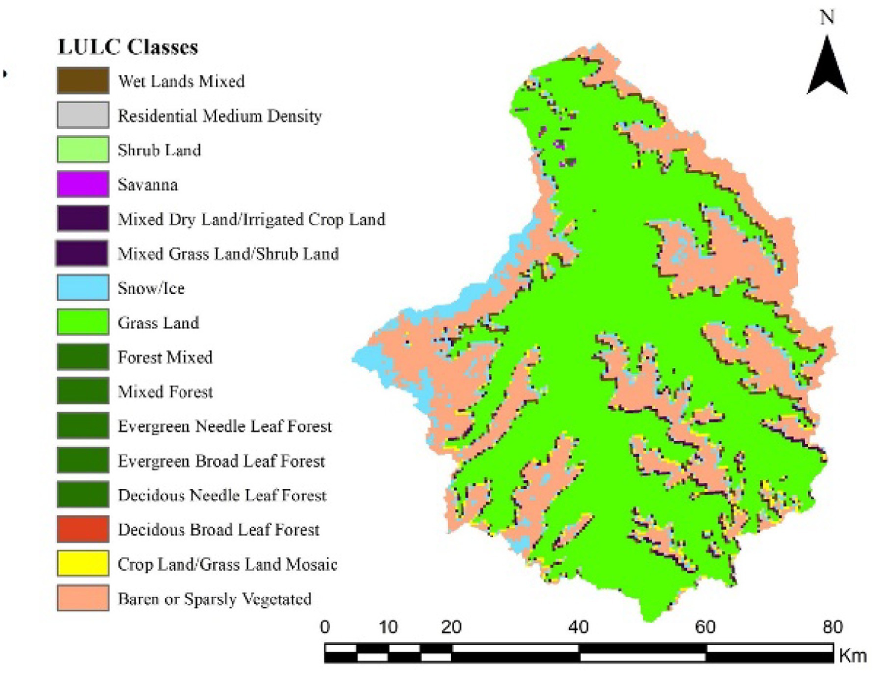
Figure 2. Description of MODIS land use classes in study area.

Figure 3

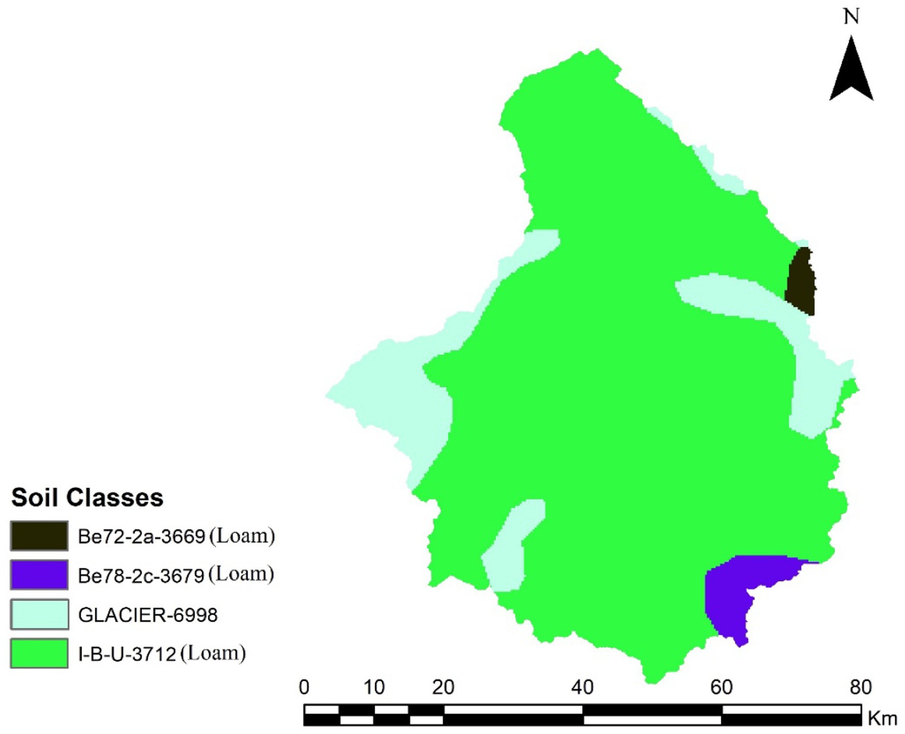
Figure 3. Description of FAO soil classes in study area.

The MODIS International Geosphere-Biosphere Program (IGBP) classification scheme provides a global land cover classification system with 17 classes, each representing a distinct land cover type. As per these classification, major classes in study area are grass land (57.23%), baren/sparsely vegetated (25.8%), snow/ice (6.51%) and others (10.46%). As per FAO, the study area consists of three loamy soils including I-B-U-3712 (83.1%), Be78-2c-3679 (2.5%), and Be72-2a-3669 (0.8%), and glaciers-6998 (13.6%). Numerous studies in the Upper Indus region have utilized the same land use and soil datasets, encountering discrepancies in the percentage of land use classes, particularly for the snow/glacier class (Haleem et al., 2023; Khan et al., 2023; Mahmood et al., 2024). A possible explanation is the difference in scales, with the FAO Soil Map of the World being developed at a much coarser scale of 1:5,000,000 compared to the finer resolution of the MODIS (500 m) land use dataset and temporal variation.

In hydroclimatic data, meteorological including daily precipitation, temperature maximum and minimum and daily streamflow data, covering the period from 2005 to 2019, were sourced from the Pakistan Meteorological Department (PMD) and the Water and Power Development Authority (WAPDA), respectively.

3.2 Model description

3.2.1 SWAT model

The SWAT is a semi-distributed hydrological model that assesses the intricate relationships between land and meteorological parameters at the watershed level (Yi and Sophocleous, 2011), formulated by Arnold et al. (1998). The main modules consist of a weather generator, water quality, hydrology and plant growth (Zhang et al., 2023). It includes spatial management practices and agricultural chemical use databases that permit the prediction of streamflows in a basin that is large and diverse in soil, land cover and management conditions (Song et al., 2022; Raihan et al., 2020). The model requires a minimal set of input data, including terrestrial information such as Digital Elevation Models (DEM), land use, and soil data, along with daily meteorological inputs like precipitation, temperature, wind speed, relative humidity, and solar radiation (Ficklin and Barnhart, 2014; Wisal et al., 2020). Due to the unavailability of observed wind speed, relative humidity, and solar radiation data, the SWAT model’s built-in weather generator was used to simulate these parameters. The weather generator estimates missing climate variables based on statistical distributions derived from historical data, ensuring that meteorological inputs remain consistent with the regional climate conditions. This approach allows for a complete dataset while maintaining the integrity of hydrological simulations.

The SWAT model divides the whole watershed into number of hydrological response units (HRUs) based on the slope, land use and soil type and simulates the spatial changes in the watershed based on the hydrological dynamics of each HRU to compute water volume in river channels (Arnold et al., 2012). It has computational capability to estimate snow and glacier melt contributions using a temperature index algorithm (TIA). Astore sub-basin was subdivided into 5 subbasins and 47 HRUs. To account for the orographic effects, each sub-catchment was split into 10 elevation bands. The SWAT model simulates hydrological processes using the Soil Conservation Service Curve Number (SCS-CN) method for runoff estimation and the Muskingum scheme for channel routing. The Penman-Monteith equation was selected to estimate evapotranspiration. Since observed wind speed, solar radiation, and relative humidity data were unavailable, the SWAT model’s built-in weather generator was used to estimate these variables based on historical climate statistics. This approach ensures that the Penman-Monteith equation remains applicable despite missing observed data. The SWAT model is founded on the principles of the water cycle, as represented in Equation 1 (Neitsch et al., 2011):

$\begin{array}{ll}S{W}_t=S{W}_0+{\displaystyle \sum _{i=1}^t}{\left(R_{\mathit{day}}+Q_{\mathit{surf}}-E_a-W_{\mathit{seep}}-Q_{gw}\right)}_i& (1)\end{array}$

Where:

SW_t: Final soil moisture content (mm).

SW₀: Initial soil moisture content on day 𝑖i (mm).

t: Time (days).

𝑅_𝑑𝑎𝑦: Precipitation on day i (mm).

𝑄_{𝑠𝑢𝑟𝑓}: Surface runoff on day i (mm).

𝐸_𝑎: Evapotranspiration on day i (mm).

𝑊_{𝑠𝑒𝑒𝑝}: Water entering the vadose zone from the soil profile on day i (mm).

${\mathrm{Q}}_{\mathrm{g}\mathrm{w}}$ : Groundwater return flow on day i (mm).

The SWAT model estimates surface runoff (𝑄_{𝑠𝑢𝑟𝑓}) using the SCS curve number method (Mockus, 1964) and Green-Ampt Infiltration method (Winchell et al., 2010). In this study, the SCS curve number method was chosen to compute surface runoff by Equation 2:

$\begin{array}{ll}{\mathrm{Q}}_{\mathrm{surf}}=\frac{{\left({\mathrm{R}}_{\mathrm{day}}-0.2\mathrm{S}\right)}^2}{\left({\mathrm{R}}_{\mathrm{day}}+0.8\mathrm{S}\right)}& (2)\end{array}$

Where Q_surf (mm) is excess rainfall or surface runoff, R_day (mm) is the rainfall in a day and S (mm per day) is the maximum retention parameter. This parameter varies spatially and temporally due to variations in land-use management, slope and soils, and soil water content, respectively. The retention parameter is given by Equation 3:

$\begin{array}{ll}\mathrm{S}=25.4\left(\frac{1000}{\mathrm{C}\mathrm{N}}-10\right)& (3)\end{array}$

Where S is defined earlier, and CN denotes the curve number.

3.2.2 BiLSTM deep learning model

The LSTM is a deep learning model type that was developed specifically to address the gradient explosion or vanish problems that traditional recurrent neural networks (RNNs) experience (Hochreiter and Schmidhuber, 1997). Over time, it has demonstrated its effectiveness in handling sequentially arranged data processing (Winchell et al., 2010; Hochreiter and Schmidhuber, 1997; Lipton et al., 2015).

During a specific time(t), a standard LSTM can solely acquire knowledge from its preceding inputs. However, through the Coupling of two LSTMs operating in opposing directions, a BiLSTM analyzes information in both forward and backward directions simultaneously, utilizing distinct hidden layers. By encompassing input information that precedes and follows each input at time t, BiLSTM exhibits the potential to outperform unidirectional LSTMs, particularly in scenarios involving time-series data. BiLSTM structure’s flow chart is demonstrated with the basic LSTM structure of cell calculation and equations in Figure 4.

Figure 4

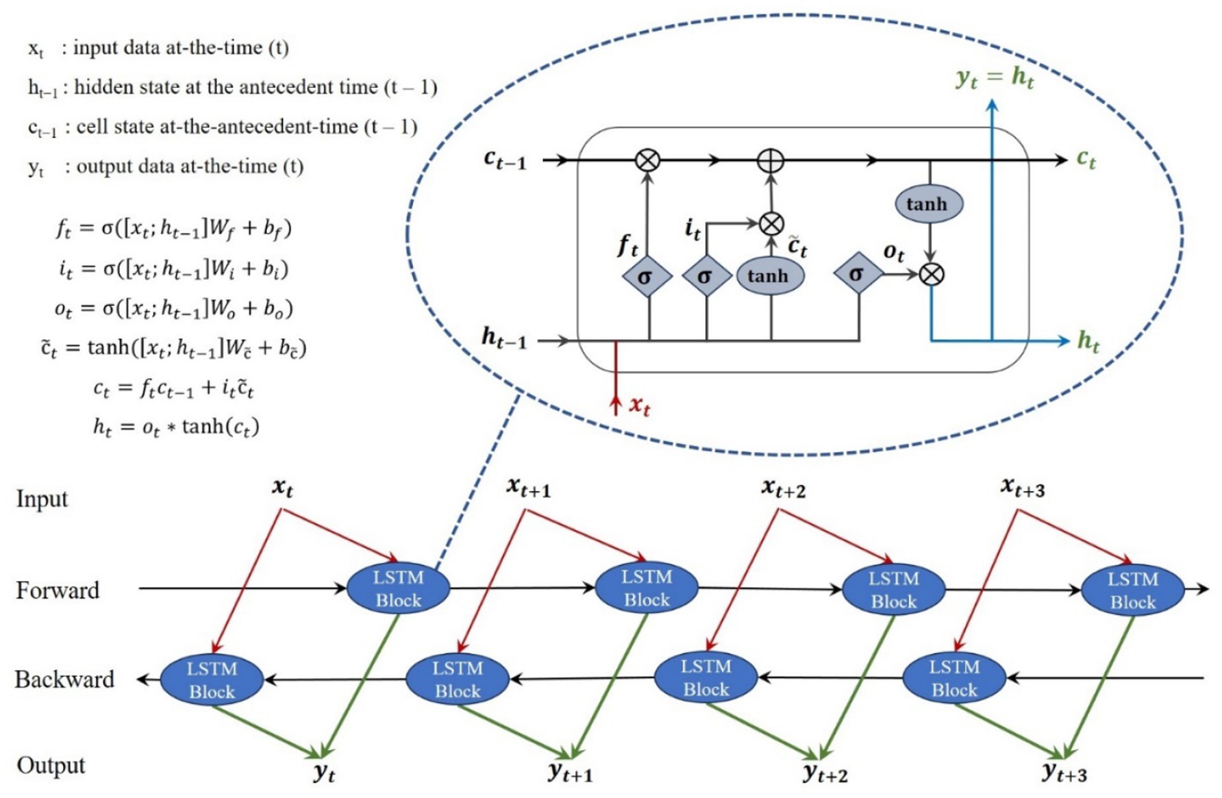
Figure 4. LSTM and BiLSTM basic structures along with equations.

The optimal architecture of the BiLSTM model was structured with careful consideration of various components to achieve peak performance and mitigate overfitting. The first hidden layer was comprised of 512 neurons, setting the foundation for subsequent layers. The following four dense layers consist of 256, 64, 32, and 1 neuron, respectively, formed a hierarchical architecture. To prevent overfitting, dropout layers with a 0.2 dropout rate were strategically placed before and after each fully connected layer (Srivastava et al., 2014).

To enhance computational efficiency and avoid gradient disappearance, the Rectified Linear Unit (ReLU) was employed as the activation function in the hidden layers (Wu et al., 2020). Compared to activation functions such as Sigmoid and Tanh, ReLU is computationally efficient, prevents vanishing gradients by allowing positive gradients to pass unchanged, and promotes faster convergence in deep networks. The optimizer of choice was Adaptive Moment Estimation (Adam), known for its adaptive learning rates and effective optimization capabilities. The learning rate was set at 0.001, contributing to the determination of the optimal combination of various hyperparameters during training.

The model’s loss function was a weighted sum of Mean Absolute Error (MAE) and Mean Square Error (MSE), allowing for a balanced evaluation of prediction errors. MAE measures absolute differences between predicted and observed values, making it robust to outliers, while MSE penalizes larger errors more heavily, encouraging the model to focus on minimizing significant deviations. The weights assigned to MAE (0.7) and MSE (0.3) were chosen to prioritize overall prediction accuracy while preventing excessive sensitivity to large errors. This combination ensures that both small and large discrepancies are accounted for in the training process, leading to improved generalization (Yang et al., 2023).

3.3 Input selection for BiLSTM standalone model

Input selection for standalone deep learning BiLSTM was carried out by cross correlation analysis to determine the most relevant meteorological factors influencing daily streamflow in the Astore sub-basin. This analysis involved computing correlation coefficients between daily streamflow and three key variables over different lag times: daily rainfall on the antecedent nth day (P_t − n), total rainfall in the preceding n days (P_n), and daily temperature on the antecedent nth day (T_t-n). These variables were chosen based on their hydrological significance, as rainfall contributes to direct runoff, cumulative rainfall accounts for delayed responses in the watershed, and temperature plays a critical role in snowmelt-driven streamflow, particularly in mountainous regions like Astore. The correlation analysis was performed for lag times ranging from 0 to 50 days, allowing the identification of the most influential time delays for each variable.

3.4 Coupling of calibrated SWAT-BiLSTM

Calibrated SWAT and BiLSTM coupling was carried out in such a way that preliminary streamflow obtained from calibrated SWAT model used as one of the inputs in data driven BiLSTM model along with the three different alternate inputs scenarios as shown in Schematic diagram of methodology (Figure 5). These scenarios were designed to explore different levels of input reliance and optimize predictive performance by integrating process-based and data-driven modeling approaches. In the SWAT-C-BiLSTM (PTQ_p) model, three input parameters were used for BiLSTM: precipitation, temperature (without any selection analysis), and preliminary flow from the calibrated SWAT model. This scenario serves as a baseline model, leveraging conventional meteorological inputs that are commonly used in hydrological modeling. The SWAT-C-BiLSTM (T₁ Q_p) model included only two input parameters: temperature with a one-day lag (based on cross-correlation analysis) and preliminary flow from the calibrated SWAT model. This scenario was developed based on cross-correlation analysis, which identified the most relevant climate variable with the highest correlation to daily streamflow. The selection of T_t−1 is particularly relevant in snowmelt-driven basins like Astore, where delayed temperature effects significantly influence streamflow. The SWAT-C-BiLSTM (Q_p) model utilized only one input parameter, the preliminary flow from the calibrated SWAT model without including precipitation or temperature. This scenario was designed to evaluate whether simulated streamflow alone, without meteorological inputs, could sufficiently drive BiLSTM predictions, effectively testing the strength of SWAT’s hydrological representation in a hybrid modeling framework.

Figure 5

Figure 5. Schematic diagram of methodology showing data collection, development of standalone models, coupling calibrated SWAT with BiLSTM under alternate inputs options, and streamflow prediction followed by statistical evaluation and ranking through compromise programing.

3.5 Calibration, validation, and prediction of models

The standalone SWAT model was calibrated and validated using the SWAT Calibration and Uncertainty Program (SWAT-CUP), following the approach of Garee et al. (2017). Model parameter uncertainty and performance were evaluated through the Sequential Uncertainty Fitting (SUFI-2) method in SWAT-CUP. To obtain the best-fit values for sensitive parameters, SWAT-CUP was run for 10,000 iterations during the calibration phase. The 2 years (2005–2006) were warm up period for model stability. Daily flow data observed at the Doyian station from 2007 to 2011 was used for calibration, while data from 2012 to 2015 served to validate the simulation results. On the other hand, based on cross correlation analysis input that was temperature at 1 day lag used as input to train and test the standalone BiLSTM data driven model at daily time scale. Keeping standalone DD model architecture same, three alternate inputs were used to train and test the models (coupled one) individually (Figure 5). Following calibration and validation, all five models including two standalone and three coupled alternate input scenarios based, were used to predict daily streamflow from 2017 to 2019.

3.6 Statistical evaluation and ranking using compromise programing

The evaluation of the each modeled daily streamflow with respect to observed daily streamflow was conducted using statistical matrices including coefficient of determination (R²), Nash Sutcliffe efficiency coefficient (NSE), percent bias (PBIAS) and root mean square error to the standard deviation ratio (RSR). Ideal value for R² and NSE is 1 while PBIAS and RSR is 0. Table 1 shows the statical matrices mathematical expression along with their possible ranges.

Table 1

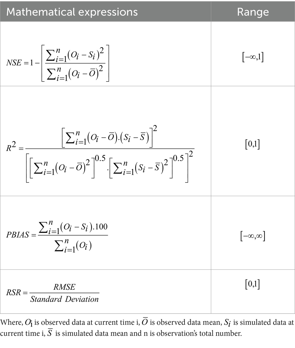
Table 1. Performance metrics describing mathematical expressions with ranges of NSE, R², PBIAS and RSR.

Compromise Programming (CP) involves combining various statistical measures, as highlighted by Iqbal et al. (2021) and Khan et al. (2023). In this study, CP was applied to assess and rank hydrological models using four core performance indicators: R², NSE, PBIAS and RSR which collectively gage the model effectiveness. Within the CP framework, researchers computed a specialized distance measure known as the L_P metric, as demonstrated by Shiru and Chung (2021). The L_P metric is defined by Equation 4:

$\begin{array}{ll}{L}_p={\left[{\displaystyle \sum _{n=1}^n}|W_n^{\ast }-W_n{|}^m\right]}^{1/m}& (4)\end{array}$

Here, the parameter m is set to 1, W_n represents the actual value of a statistical performance measure, and ${\mathrm{W}}_{\mathrm{n}}^{\ast }$ denotes the ideal value of the performance measure achieved when model simulations perfectly align with observed data. The L_p metric is always positive, and lower L_p values are preferred as they signify superior model performance.

4 Results

This section includes results description of the selection of the input for standalone data driven model, calibration and validation performance of models, prediction performance and lastly ranking using compromise programing based on statistical evaluations.

4.1 Selection for standalone data driven model input

Input selection for deep learning standalone BiLSTM model was carried out by cross correlation analysis. Figure 6 illustrates the correlation coefficients between daily streamflow and daily rainfall, total rainfall and temperature factors, respectively, at daily lag time from 2005 to 2015. These factors include daily rainfall on the antecedent nth day (P_t − n), total rainfall in the preceding n days (P_n), and daily temperature on the antecedent nth day (T_t-n). The maximum daily rainfall and total rainfall exhibited correlations of 0.12 and 0.10, respectively. In contrast, the analysis showed that the temperature on the preceding day (T_t-1) had the highest correlation of 0.69 with the basin’s daily streamflow. As a result, T_t-1 was chosen as the covariate in the BiLSTM model to simulate daily streamflow in the Astore sub-basin.

Figure 6

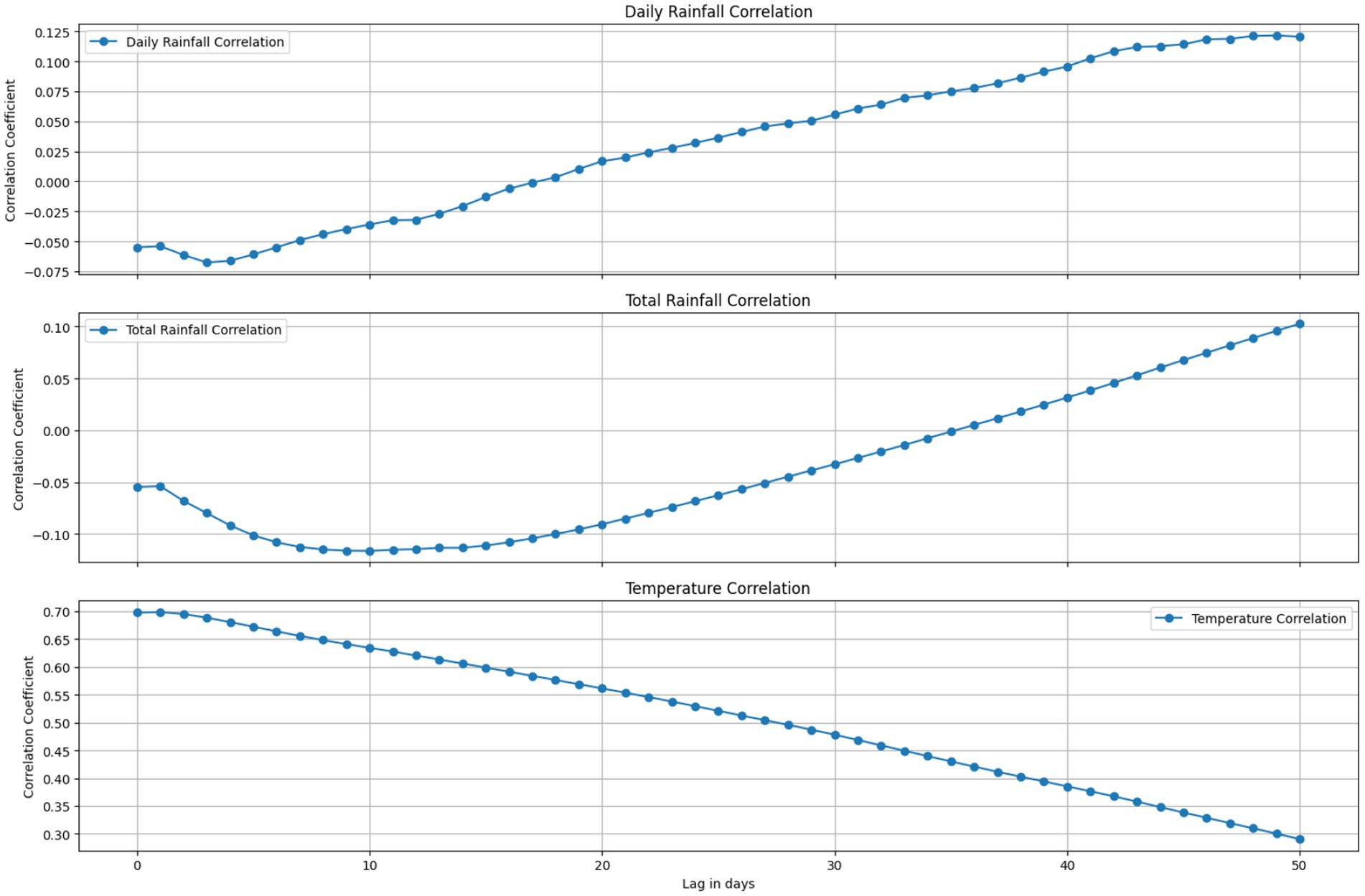
Figure 6. Cross correlation analysis between daily streamflow and daily rainfall on the previous nth day, total rainfall in the preceding n-days and daily temperature on the previous nth day, respectively in Astore basin for the duration 2005–2015.

4.2 Sensitivity analysis, calibration, and validation performances of models

The performance of the two standalone models (SWAT and BiLSTM) and three coupled models (SWAT-C-BiLSTM (T₁Q_p), SWAT-C-BiLSTM (Q_p), and SWAT-C-BiLSTM (PTQ_p)) was evaluated during the calibration (2007–2011) and validation (2012–2015) periods at the Doyian station on the Astore River. A warm-up period of 2 years (2005–2006) was used to stabilize the physically based SWAT model.

Sensitivity analysis was conducted during SWAT model calibration and 24 parameters were identified as critical for simulating daily streamflows, as presented in Table 2 and their ranges and fitted values are presented in Figure 7. Table 2 also presents the t-test values and p-values derived from Global Sensitivity Analyses for selected parameters in the Astore sub-basin. Among these, groundwater-related parameters, including ALPHA_BF (baseflow recession coefficient), GW_DELAY (groundwater delay time), GWQMN (threshold depth of water in the shallow aquifer required for return flow), and REVAPMN (threshold depth of water in the shallow aquifer for percolation to deep aquifers), played a crucial role in regulating baseflow contributions to the river. These parameters influenced model performance, particularly in low-flow conditions, highlighting the potential interactions between surface water and groundwater in the basin.

Figure 7

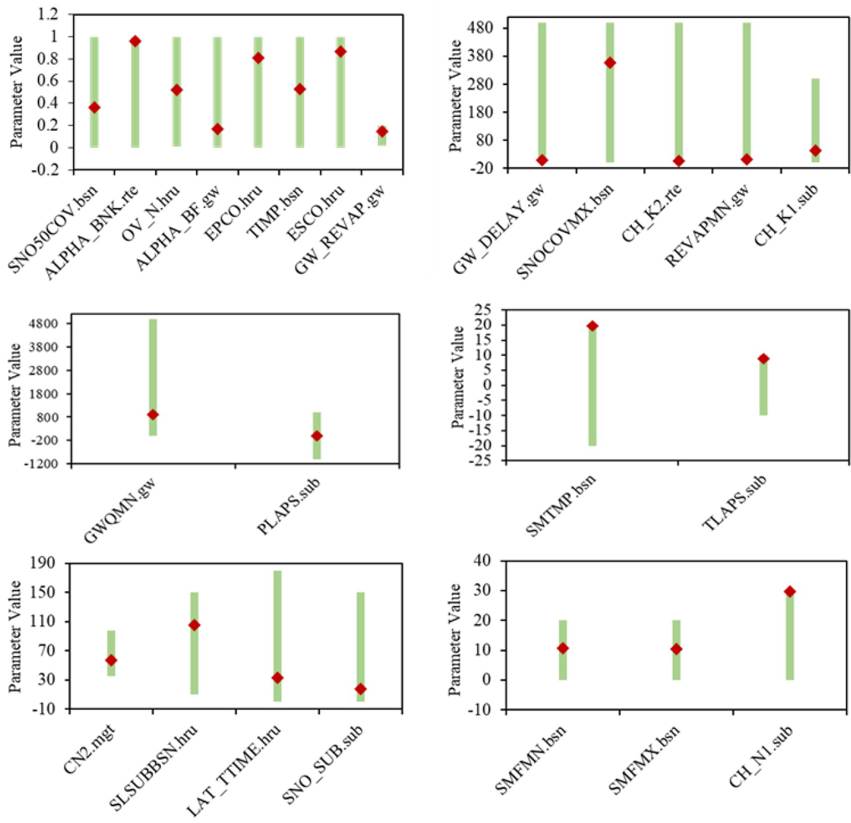
Figure 7. Parameters utilized in standalone SWAT model for calibration showing light green range (minimum and maximum) bar and dark red fitted values.

Table 2

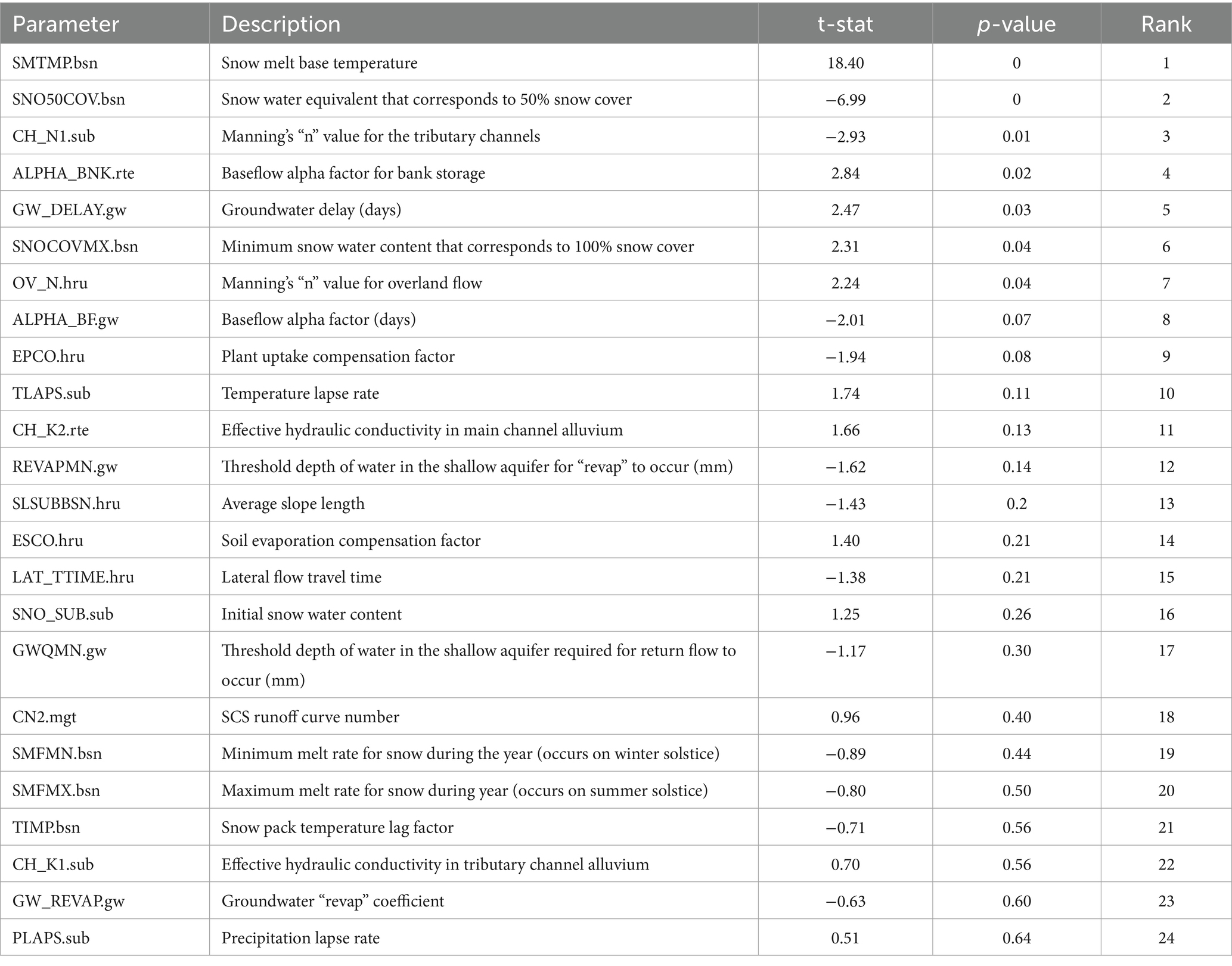
Table 2. Sensitive parameters during SWAT model calibration with t-stat, p-value, and ranks.

The most sensitive parameters, SMTMP, SNO50COV, and CH_N1, were crucial for calibrating the SWAT-T-BiLSTM model. In this area, snow cover and glacier melt are the primary water sources (Ayub et al., 2020; Ali et al., 2023), which explains SWAT’s sensitivity to SMTMP (snowmelt base temperature) and SNO50COV (snow water equivalent at 50% snow cover). Additionally, sub-basin, hydraulic response unit, and groundwater parameters significantly influenced streamflow simulations.

While groundwater parameters were considered during calibration, direct observational evidence of river-aquifer interactions in the Astore basin is limited. Future studies incorporating hydrogeological field measurements, isotopic analysis, or groundwater monitoring networks could further improve the constraint on these parameters and enhance the model’s physical realism.

During the calibration (2007–2011) and validation (2012–2015) phases, the coupled models outperformed the standalone models in both statistical metrics (Figure 8) and flow simulation (Table 3). Among the coupled models, SWAT-C-BiLSTM (T₁Q_p) and SWAT-C-BiLSTM (Q_p) exhibited comparable performance, demonstrating superior accuracy in streamflow prediction. SWAT-C-BiLSTM (Q_p) achieved an NSE of 0.73 and 0.78, an R² of 0.83 and 0.85, and a low PBIAS of 23.78 and 21.74% during calibration and validation periods, respectively. Similarly, SWAT-C-BiLSTM (T₁Q_p) showed an NSE of 0.80 and 0.73, R² of 0.89 and 0.84, and effectively replicated low flows with averages of 32.54 m³/s and 32.65 m³/s. Both models effectively captured peak and low flows, with SWAT-C-BiLSTM (T₁Q_p) slightly better at simulating peak flows, while SWAT-C-BiLSTM (Q_p) exhibited slightly lower bias in terms of PBIAS. Given their close performance, both models can be considered equally robust for accurate daily streamflow predictions. Line plots of calibration and validation are shown in Figures 9, 10.

Figure 8

Figure 8. Statistical evaluation of different models during calibration/training, validation/testing, and prediction phase by utilizing R², NSE, PBIAS, and RSR, respectively.

Table 3

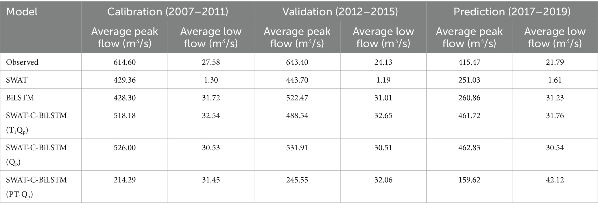
Table 3. Yearly average of daily peak and low flows summary during calibration, validation, and prediction phases, observed and simulated by different models.

Figure 9

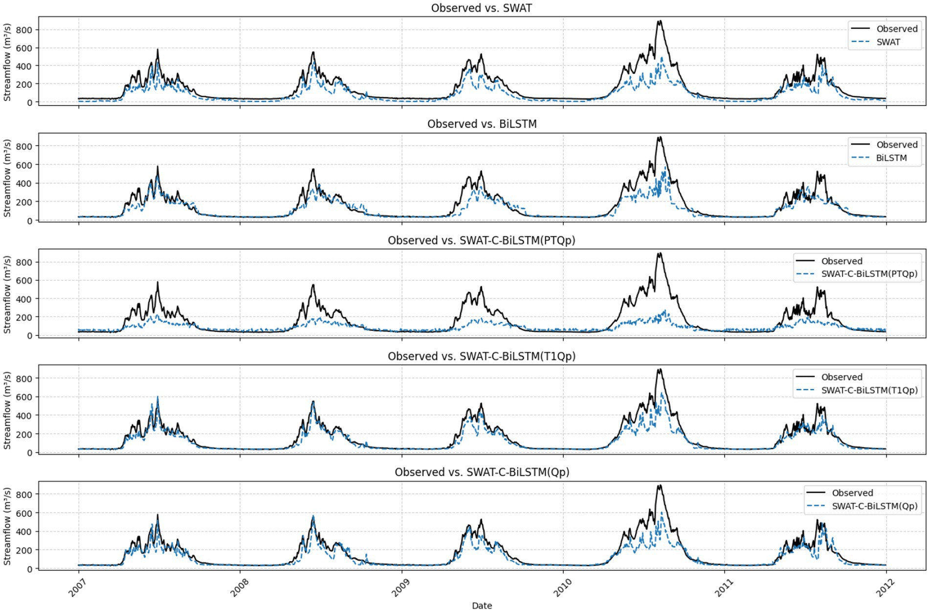
Figure 9. Calibration/training of standalone and coupled models under alternate input options at daily time scale.

Figure 10

Figure 10. Validation/testing of standalone and coupled models under alternate inputs options at daily time scale.

In contrast, the standalone SWAT model exhibited significant biases, with PBIAS exceeding 44 and 48.26% and showed a tendency to underestimate both peak and low flows, as reflected in the low flow averages of 1.30 m³/s and 1.19 m³/s compared to the observed values of 27.58 m³/s and 24.13 m³/s (Table 3). The standalone BiLSTM model performed better than SWAT, achieving an NSE of 0.67 and 0.68, and producing low flows average of 31.72 m³/s and 31.01 m³/s, yet it still lagged behind coupled models. Among the coupled models, SWAT-C-BiLSTM (PT₁Q_p) performed the weakest, likely due to uncertainties in precipitation and temperature inclusion, resulting in low NSE values of 0.23 and 0.27 and a higher PBIAS of 31.45 and 32.06%. These results highlight the superiority of SWAT-C-BiLSTM (Q_p) and SWAT-C-BiLSTM (T₁Q_p) in accurately predicting both high and low flows, with no significant advantage over the other, making both valuable tools for hydrological modeling (Table 4).

Table 4

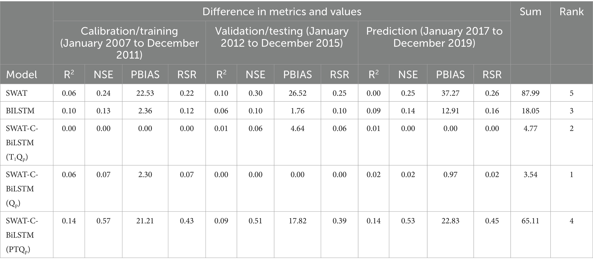
Table 4. Difference in metrics and values for ranking of models using compromise programing approach.

4.3 Model prediction performance

During the prediction period (2017–2019), the coupled models continued to outperform the standalone models in terms of statistical metrics and flow simulation accuracy (Figure 11a and Table 4). SWAT-C-BiLSTM (T₁Q_p) and SWAT-C-BiLSTM (Q_p) exhibited nearly identical predictive capabilities, with SWAT-C-BiLSTM (T₁Q_p) achieving an NSE of 0.88 and R² of 0.89, while SWAT-C-BiLSTM (Q_p) attained an NSE of 0.86 and R² of 0.87. Both models effectively minimized bias, with PBIAS values of 4.06 and 5.04%, respectively. These models demonstrated high accuracy in capturing streamflow variations, including peak and low flows, with SWAT-C-BiLSTM (T₁Q_p) showing slightly better peak flow predictions, whereas SWAT-C-BiLSTM (Q_p) maintained lower bias in overall flow representation.

Figure 11

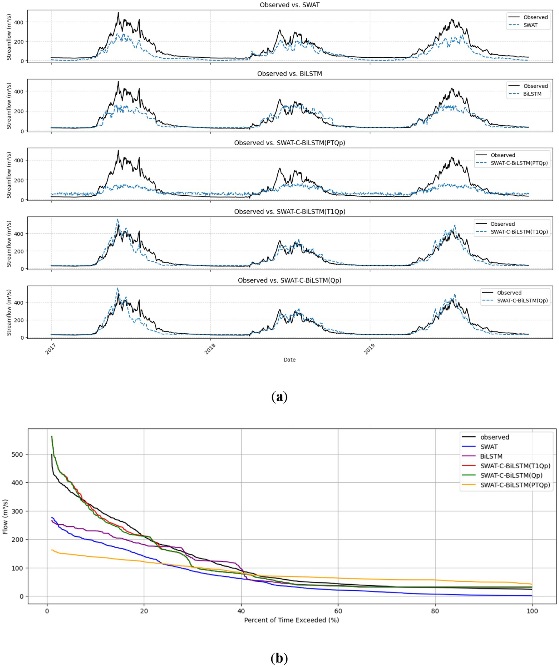
Figure 11. (a) Prediction of standalone and coupled models under alternate input options at daily time scale for streamflow simulation; (b) flow duration curve during prediction phase.

In contrast, the standalone SWAT model exhibited considerable bias, reflected in its high PBIAS of 41.33% and lower NSE of 0.62. It significantly underestimated both peak and low flows, with an average peak flow of 251.03 m³/s compared to the observed 415.47 m³/s and an average low flow of 1.61 m³/s against the observed 21.79 m³/s. On the other hand, SWAT-C-BiLSTM (Q_p) closely matched the observed peak flow with 462.83 m³/s, while its low flow predictions (30.54 m³/s) remained highly consistent with the observed values. SWAT-C-BiLSTM (T₁Q_p) followed a similar trend, maintaining comparable accuracy across different flow conditions.

Among the coupled models, SWAT-C-BiLSTM (PT₁Q_p) performed the weakest, likely due to increased uncertainty from additional climate inputs, resulting in the highest bias in low flow predictions (42.12 m³/s). The flow duration curve (Figure 11b) further illustrates that SWAT-C-BiLSTM (T₁Q_p) and SWAT-C-BiLSTM (Q_p) closely follow the observed flow distribution across different exceedance probabilities, reinforcing their reliability in predictive performance. These findings highlight the effectiveness of coupled models, particularly SWAT-C-BiLSTM (T₁Q_p) and SWAT-C-BiLSTM (Q_p), in accurately simulating streamflow across different hydrological conditions.

4.4 Model ranking using the CP approach based on statistical evaluation

The CP approach effectively evaluated the performance of the models by aggregating statistical metrics into a single ranking criterion, allowing for a holistic comparison across calibration, validation, and prediction periods. The rankings (Table 4) identified SWAT-C-BiLSTM (Q_p) as the best-performing model, achieving the lowest aggregate (3.54) due to its consistent superiority across all metrics, particularly during validation and prediction periods. It exhibited minimal differences in R², NSE, PBIAS, and RSR compared to observed values, reflecting its robust ability to capture both peak and low flow dynamics. Similarly, SWAT-C-BiLSTM (T₁Q_p) secured the second rank with an aggregate of 4.77, demonstrating competitive performance, although slightly less accurate than SWAT-C-BiLSTM (Q_p) in some scenarios.

In contrast, the standalone SWAT model ranked at last (87.99), with the highest aggregate metric deviations, emphasizing its limitations in simulating streamflow under complex hydrological conditions. The BiLSTM model with an aggregate of 18.05 ranked at third 18.05, performing well independently but falling behind the coupled models due to its lack of physical hydrological considerations. The SWAT-C-BiLSTM (PTQ_p) model ranked at fourth having an aggregate of 65.11, primarily due to higher discrepancies in PBIAS and RSR, which impacted on its overall performance.

These results underscore the efficiency of the CP approach in ranking models, affirming the superiority of coupled models SWAT-C-BiLSTM (Q_p) and SWAT-C-BiLSTM (T₁Q_p) for streamflow prediction. This ranking provides a clear decision-making framework for selecting models tailored to high-performance hydrological simulations at daily timescale.

5 Discussion

5.1 Results interpretation and comparison

The coupled SWAT-C-BiLSTM (Q_p) model, excluding climatic variables as inputs to BiLSTM, and The cross correlation-based coupling scenario, SWAT-C-BiLSTM (T₁ Q_p), emerged as the best-performing scenarios in this study, achieving the highest accuracy and lowest bias in streamflow prediction. Conversely, SWAT-C-BiLSTM (PTQ_P), which included both precipitation and temperature, performed the poorest. These findings highlight the critical role of optimized input selection in enhancing the performance of hybrid hydrological models.

The SWAT-C-BiLSTM (Q_p) model does not explicitly incorporate climate variables such as temperature and precipitation as direct inputs to BiLSTM, these variables are inherently embedded within the SWAT-simulated flow (Q_p). SWAT is a process-based model that simulates streamflow based on climatic inputs, land surface interactions, and catchment hydrological processes. Thus, Q_p inherently carries the aggregated influence of precipitation, temperature, and other hydrological drivers. Our results indicate that using Q_p as an input to BiLSTM allows for leveraging SWAT’s physically based outputs while reducing additional uncertainties that may arise from directly incorporating climate variables into BiLSTM. This does not mean that temperature and other climatic factors are disregarded; rather, their effects are already encapsulated in the Q_p variable as simulated by SWAT.

The findings are align with the study Jeong D. S. et al. (2024), where the inclusion of climate variable precipitation to hybrid models did not make noticeable improvements for streamflow and suspended solids simulations. Additionally, the coupled models performed better compared to standalone SWAT and data driven models (Yang et al., 2023; Jeong H. et al., 2024; Mei et al., 2024). Daily temperature showed a stronger correlation with streamflow than precipitation, reflecting the snow and glacier melt dominated hydrology of the Astore sub-basin. This may be attributed to the fact that streamflow in the study area is primarily driven by glacier melt, followed by snowmelt and rainfall (Ayub et al., 2020; Ali et al., 2023).

The relatively poor performance of the standalone SWAT model, as observed in this study, can be attributed to several factors, including limited observed climate data and the reliance on default settings for critical variables like relative humidity, wind speed, and solar radiation. Ghane and Alvankar (2015) highlight how variations in these parameters can drastically influence runoff estimations, underscoring the importance of accurate meteorological inputs. Furthermore, the inadequate coverage of rain gages and the coarse resolution data likely exacerbate uncertainties, as demonstrated by Anderson and Bingner (2010) and Gao et al. (2017), respectively. The SWAT model may struggle to accurately identify the most sensitive parameters (Shen et al., 2008; Cibin et al., 2010), including snow-specific parameters, for each sub-basin due to the coarse resolution of land use data, which hinders its ability to capture unique sub-basin conditions. High-resolution datasets and improved spatial coverage could address these limitations and enhance the model’s ability to capture sub-basin characteristics. Additionally, the lack of preprocessing and calibration for snow-specific parameters may have compounded these challenges, consistent with findings by Jajarmizadeh et al. (2017). In future work, leveraging alternative data sources such as Climate Forecast System Reanalysis (CFSR) etc. in place of default SWAT algorithm should be utilized as Haleem et al. (2023) and employing advanced calibration techniques may improve model performance and reduce uncertainties in hydrological predictions.

These limitations are mitigated by coupling SWAT with BiLSTM, which provides enhanced flexibility and adaptability in modeling nonlinear hydrological processes. The BiLSTM model, in this study, demonstrated its capacity to adapt to dominant hydrological drivers, such as glaciers and snowmelt, effectively capturing low-flow conditions across all phases. However, as a standalone model, BiLSTM faced challenges in simulating peak flows due to the absence of physical process representation.

In SWAT-C-BiLSTM (Q_p) scenario, BiLSTM leveraged SWAT’s physically based outputs to significantly improve peak flow simulations while addressing uncertainties associated with coarse-resolution land use data and limited climatic variables. This coupling approach underscores the complementary strengths of BiLSTM, with selective variable integration playing a pivotal role. Additionally, since SWAT simulates streamflow by incorporating these climatic variables, the coupled scenarios we discuss pertain specifically to BiLSTM’s input selection and do not imply that the SWAT-simulated flow (Q_p) is devoid of climatic influences.

The marginal accuracy difference between the excluded-variable scenario (SWAT-C-BiLSTM (Q_p)) and the cross correlation based included variable scenario (SWAT-C-BiLSTM (T₁ Q_p)) highlights the importance of carefully curating input variables rather than including all climatic data. For glacier-fed basins like Astore, where precipitation has limited daily correlation with streamflow, excluding it from the coupling process yielded enhanced performance.

5.2 Implications for hydrology and model development

The findings of this study underscore the critical importance of optimizing input selection and leveraging hybrid modeling approaches in hydrology. The superior performance of the SWAT-C-BiLSTM (Q_p) scenario, which excluded climatic variables from direct BiLSTM input, demonstrates that selective integration of variables aligned with dominant hydrological drivers can enhance model accuracy while reducing uncertainty. This is particularly relevant for glacier-fed basins like Astore, where streamflow is primarily influenced by glacier and snowmelt rather than precipitation. The results highlight the complementary strengths of physically based models, like SWAT, and data-driven approaches, such as BiLSTM, in addressing the limitations of standalone models. By combining physical process representation with nonlinear adaptability, coupled models offer a promising pathway for improving hydrological predictions in data-scarce and complex environments, paving the way for more robust water resource management strategies under changing climatic conditions.

5.3 Operational relevance for water resource management

The findings of this study offer practical implications for water resource management, particularly in streamflow forecasting for flood and drought preparedness. The superior performance of the SWAT-C-BiLSTM (Q_p) model suggests that integrating process-based hydrological models with machine learning can enhance predictive accuracy without requiring direct climate inputs. This is particularly beneficial in data-scarce regions where real-time climate data may be limited.

Improved streamflow predictions can aid water managers in optimizing reservoir operations, flood risk mitigation, and drought preparedness by providing more reliable forecasts. The study’s approach could be further explored for operational hydrological forecasting systems, ensuring robust water resource planning under changing climatic conditions.

5.4 Limitations and future directions

This study faced several limitations that could influence the outcomes. The use of coarse resolution land use data, such as MODIS, introduced uncertainties in sub-basin parameterization, potentially affecting the accuracy of hydrological simulations. Limited preprocessing of hydroclimatic data impacted the ability to accurately simulate peak and low-flow conditions. The reliance on cross-correlation for lag selection between climatic variables, while effective as a preliminary step, may not fully capture the nonlinear relationships inherent in hydrological processes, potentially leading to suboptimal lag time identification. Additionally, considering only precipitation and temperature as climatic variables may not fully capture the hydrological complexities of the Astore sub-basin, particularly in a glacier-fed system. Also, the findings are specific to the Astore sub-basin, and their generalizability to other regions with varying geographic and climatic contexts remains unexplored.

Meteorological data were obtained from the Pakistan Meteorological Department (PMD) and the Water and Power Development Authority (WAPDA); however, these datasets may have limited spatial coverage. Future studies could explore the use of alternative data sources, such as ERA5 or Climate Forecast System Reanalysis (CFSR) datasets, to supplement observed meteorological inputs and potentially enhance model accuracy. The integration of high-resolution reanalysis datasets could improve spatial representation and reduce uncertainties in hydrological simulations, particularly in data-scarce mountainous regions.

Additionally, while groundwater parameters were considered during calibration, direct observational evidence of river-aquifer interactions in the Astore sub-basin is limited. Future studies incorporating hydrogeological field measurements, isotopic analysis, or groundwater monitoring networks could further improve the constraint on these parameters and enhance the model’s physical realism. Groundwater contributions, particularly in low-flow conditions, may play a more significant role than currently represented in the model, warranting further investigation.

Moreover, future studies should incorporate high-resolution land use data to enhance parameter sensitivity and simulation accuracy. Expanding the range of climatic inputs to include additional variables, such as precipitation variables, humidity and solar radiation, could provide a more comprehensive understanding of hydrological processes. Incorporating more robust and exhaustive methods, such as cross-validation, grid search, or advanced feature selection techniques, is recommended to systematically optimize lag times and better align with the nonlinear capabilities of machine learning models. Thorough preprocessing of hydroclimatic data is critical to minimize uncertainties, especially for extreme events. Additionally, testing the exclusion or inclusion approach in diverse geographic and climatic regions will help assess its broader applicability and effectiveness in coupled modeling scenarios.

6 Conclusion

This study explored alternate coupling inputs of a data-driven model to enhance daily streamflow prediction in a calibrated SWAT-BiLSTM rainfall-runoff modeling framework for the Astore sub-basin of the Upper Indus Basin, Pakistan. Five modeling scenarios were analyzed, including standalone SWAT and BiLSTM models and three alternate coupling configurations that utilized conventional climate variables (precipitation and temperature), cross-correlation-based variable selection (temperature or precipitation), and a scenario excluding direct climatic inputs while incorporating SWAT-simulated streamflow. Model calibration, validation, and prediction were conducted for the periods January 2007 to December 2011, January 2012 to December 2015, and January 2017 to December 2019, respectively. Model performance was evaluated using statistical metrics (R², NSE, PBIAS, and RSR), and a ranking was established through Compromise Programming. The key findings of this study are as follows:

Cross-correlation analysis identified temperature as the most influential input (maximum correlation of 0.69 at 1-day lag), emphasizing the need for optimized input selection in coupled modeling.

The SWAT-C-BiLSTM (Q_p) model, which excluded direct climate inputs, emerged as the best-performing configuration, followed closely by the cross correlation based SWAT-C-BiLSTM (T₁Q_p) model. These models exhibited minimal bias and high predictive accuracy.

The compromise programming ranking confirmed the superiority of coupled models, except for SWAT-C-BiLSTM (PTQ_p), over standalone SWAT and BiLSTM models, demonstrating the benefits of integrating physically based and machine-learning approaches.

Data availability statement

The spatial data used in this study including elevation, land use and soil data is freely available and can be accessed from the websites given in the data section of the manuscript. The climatic parameters and stream flow data is the property of the Pakistan Meteorological Department (PMD) and Water and Power Development Authority (WAPDA), Pakistan, respectively, and can be requested from these departments via official channels. The data that support the findings of this study are available on request from the corresponding author.

Author contributions

KA: Conceptualization, Formal analysis, Investigation, Methodology, Validation, Visualization, Writing – original draft, Writing – review & editing. MI: Conceptualization, Formal analysis, Investigation, Methodology, Supervision, Writing – review & editing. MT: Conceptualization, Formal analysis, Investigation, Validation, Writing – review & editing. AK: Conceptualization, Formal analysis, Investigation, Validation, Writing – review & editing. AN: Formal analysis, Investigation, Validation, Visualization. JC: Formal analysis, Resources, Validation, Writing – review & editing, Funding acquisition. KU: Funding acquisition, Investigation, Methodology, Project administration. HamA: Formal analysis, Investigation, Validation, Visualization, Resources. HasA: Conceptualization, Funding acquisition, Supervision, Writing – review & editing. MA: Validation, Investigation, Methodology, Writing – review & editing.

Funding

The author(s) declare that financial support was received for the research and/or publication of this article. The research is partially funded by Gansu Provincial Science and Technology Program (25JRRA510), the program of the State Key Laboratory of Cryospheric Science and Frozen Soil Engineering, Chinese Academy of Sciences (CSFSE-ZQ-2411) and the Young Elite Scientists Sponsorship Program by CAST (2023QNRC001), the Ministry of Science and Higher Education of the Russian Federation as part of the World-class Research Center program Advanced Digital Technologies [contract no. 075-15-2022 (contract no. 075-15-311 dated 20.04.2022)]. This research was also funded by Taif University, Saudi Arabia (project no. TU-DSPP-2024-33).

Acknowledgments

The authors are grateful to the Center of Excellence in Water Resources Engineering, UET Lahore, for supporting this study. They also extend their gratitude to the Pakistan Meteorological Department (PMD) and the Water and Power Development Authority (WAPDA), Pakistan, for providing the observed meteorological and hydrological data used in this study. Additionally, the authors sincerely thank the reviewers for their invaluable insights, which have significantly improved the quality of the manuscript.

Conflict of interest

The authors declare that the research was conducted in the absence of any commercial or financial relationships that could be construed as a potential conflict of interest.

Generative AI statement

The authors declare that no Gen AI was used in the creation of this manuscript.

Publisher’s note

All claims expressed in this article are solely those of the authors and do not necessarily represent those of their affiliated organizations, or those of the publisher, the editors and the reviewers. Any product that may be evaluated in this article, or claim that may be made by its manufacturer, is not guaranteed or endorsed by the publisher.

References

Afshan, N. S., Khalid, A. N., Iqbal, S. H., Niazi, A. R., and Sultan, A. (2009). Puccinia subepidermalis Sp. Nov. and new records of rust fungi from fairy meadows, northern Pakistan. Mycotaxon 110, 173–182. doi: 10.5248/110.173

Crossref Full Text | Google Scholar

Ali, Z., Iqbal, M., Khan, I. U., Masood, M. U., Umer, M., Lodhi, M. U. K., et al. (2023). Hydrological response under CMIP6 climate projection in Astore River basin, Pakistan. J. Mt. Sci. 20, 2263–2281. doi: 10.1007/s11629-022-7872-x

Crossref Full Text | Google Scholar

Anderson, M., and Bingner, R. L. (2010). Impact of precipitation uncertainty on Swat model performance.

Google Scholar

Arnold, J. G., Moriasi, D. N., Gassman, P. W., Abbaspour, K. C., White, M. J., Srinivasan, R., et al. (2012). SWAT: model use, calibration, and validation. Trans. ASABE 55, 1491–1508. doi: 10.13031/2013.42256

Crossref Full Text | Google Scholar

Arnold, J. G., Srinivasan, R., Muttiah, R. S., and Williams, J. R. (1998). Large area hydrologic modeling and assessment part I: model development 1. JAWRA 34, 73–89. doi: 10.1111/j.1752-1688.1998.tb05961.x

Crossref Full Text | Google Scholar

Ayub, S., Akhter, G., Ashraf, A., and Iqbal, M. (2020). Snow and glacier melt runoff simulation under variable altitudes and climate scenarios in Gilgit River basin, Karakoram region. Modeling Earth Syst. Environ. 6, 1607–1618. doi: 10.1007/s40808-020-00777-y

Crossref Full Text | Google Scholar

Bizuneh, B. B., Moges, M. A., Sinshaw, B. G., and Kerebih, M. S. (2021). SWAT and HBV models’ response to streamflow estimation in the upper Blue Nile Basin, Ethiopia. Water-Energy Nexus 4, 41–53. doi: 10.1016/j.wen.2021.03.001

Crossref Full Text | Google Scholar

Chen, S., Huang, J., and Huang, J.-C. (2023). Improving daily streamflow simulations for data-scarce watersheds using the coupled SWAT-LSTM approach. J. Hydrol. 622:129734. doi: 10.1016/j.jhydrol.2023.129734

Crossref Full Text | Google Scholar

Cheng, M., Fang, F., Kinouchi, T., Navon, I. M., and Pain, C. C. (2020). Long Lead-time daily and monthly streamflow forecasting using machine learning methods. J. Hydrol. 590:125376. doi: 10.1016/j.jhydrol.2020.125376

Crossref Full Text | Google Scholar

Cibin, R., Sudheer, K. P., and Chaubey, I. (2010). Sensitivity and identifiability of stream flow generation parameters of the SWAT model. Hydrol. Proc. Int. J. 24, 1133–1148. doi: 10.1002/hyp.7568

Crossref Full Text | Google Scholar

Cui, F., Salih, S. Q., Choubin, B., Bhagat, S. K., Samui, P., and Yaseen, Z. M. (2020). Newly explored machine learning model for river flow time series forecasting at Mary River, Australia. Environ. Monit. Assess. 192, 1–15. doi: 10.1007/s10661-020-08724-1

PubMed Abstract | Crossref Full Text | Google Scholar

Dakhlalla, A. O., and Parajuli, P. B. (2019). Assessing model parameters sensitivity and uncertainty of streamflow, sediment, and nutrient transport using SWAT. Inf. Proc. Agric. 6, 61–72. doi: 10.1016/j.inpa.2018.08.007

Crossref Full Text | Google Scholar

Fan, H., Jiang, M., Ligang, X., Zhu, H., Cheng, J., and Jiang, J. (2020). Comparison of long short term memory networks and the hydrological model in runoff simulation. Water 12:175. doi: 10.3390/w12010175

Crossref Full Text | Google Scholar

Farhan, S. B., Zhang, Y., Ma, Y., Guo, Y., and Ma, N. (2015). Hydrological regimes under the conjunction of westerly and monsoon climates: a case investigation in the Astore Basin, northwestern Himalaya. Clim. Dyn. 44, 3015–3032. doi: 10.1007/s00382-014-2409-9

Crossref Full Text | Google Scholar

Ficklin, D. L., and Barnhart, B. L. (2014). SWAT hydrologic model parameter uncertainty and its implications for Hydroclimatic projections in snowmelt-dependent watersheds. J. Hydrol. 519, 2081–2090. doi: 10.1016/j.jhydrol.2014.09.082

Crossref Full Text | Google Scholar

Gao, J., Sheshukov, A. Y., Yen, H., and White, M. J. (2017). Impacts of alternative climate information on hydrologic processes with SWAT: a comparison of NCDC, PRISM and NEXRAD datasets. Catena 156, 353–364. doi: 10.1016/j.catena.2017.04.010

Crossref Full Text | Google Scholar

Garee, K., Chen, X., Bao, A., Wang, Y., and Meng, F. (2017). Hydrological modeling of the upper Indus Basin: a case study from a high-altitude Glacierized catchment Hunza. Water 9:17. doi: 10.3390/w9010017

Crossref Full Text | Google Scholar

Gassman, P. W., Reyes, M. R., Green, C. H., and Arnold, J. G. (2007). The soil and water assessment tool: historical development, applications, and future research directions. Trans. ASABE 50, 1211–1250. doi: 10.13031/2013.23637

Crossref Full Text | Google Scholar

Ghaith, M., and Li, Z. (2020). Propagation of parameter uncertainty in SWAT: a probabilistic forecasting method based on polynomial Chaos expansion and machine learning. J. Hydrol. 586:124854. doi: 10.1016/j.jhydrol.2020.124854

Crossref Full Text | Google Scholar

Ghane, M., and Alvankar, S. R. (2015). Sensitivity analysis of meteorological parameters in runoff modelling using SWAT (case study: Kasillian watershed). J. Water Sci. Res. 7, 63–78.

Google Scholar

Ghasemlounia, R., Gharehbaghi, A., Ahmadi, F., and Saadatnejadgharahassanlou, H. (2021). Developing a novel framework for forecasting groundwater level fluctuations using bi-directional long short-term memory (BiLSTM) deep neural network. Comput. Electron. Agric. 191:106568. doi: 10.1016/j.compag.2021.106568

Crossref Full Text | Google Scholar

Haleem, K., Khan, A. U., Ahmad, S., Khan, M., Khan, F. A., Khan, W., et al. (2022). Hydrological impacts of climate and land-use change on flow regime variations in upper Indus Basin. J. Water Clim. Change 13, 758–770. doi: 10.2166/wcc.2021.238

Crossref Full Text | Google Scholar

Haleem, K., Khan, A. U., Khan, J., Ghanim, A. A. J., and Al-Areeq, A. M. (2023). Evaluating future streamflow patterns under SSP245 scenarios: insights from CMIP6. Sustain. For. 15:16117. doi: 10.3390/su152216117

Crossref Full Text | Google Scholar

Hochreiter, S., and Schmidhuber, J. (1997). Long short-term memory. Neural Comput. 9, 1735–1780. doi: 10.1162/neco.1997.9.8.1735

PubMed Abstract | Crossref Full Text | Google Scholar

Hu, C., Qiang, W., Li, H., Jian, S., Li, N., and Lou, Z. (2018). Deep learning with a long short-term memory networks approach for rainfall-runoff simulation. Water 10:1543. doi: 10.3390/w10111543

Crossref Full Text | Google Scholar

Huang, S., Eisner, S., Magnusson, J. O., Lussana, C., Yang, X., and Beldring, S. (2019). Improvements of the spatially distributed hydrological modelling using the HBV model at 1 km resolution for Norway. J. Hydrol. 577:123585. doi: 10.1016/j.jhydrol.2019.03.051

Crossref Full Text | Google Scholar

Iqbal, Z., Shahid, S., Ahmed, K., Ismail, T., Ziarh, G. F., Chung, E.-S., et al. (2021). Evaluation of CMIP6 GCM rainfall in mainland Southeast Asia. Atmos. Res. 254:105525. doi: 10.1016/j.atmosres.2021.105525

Crossref Full Text | Google Scholar

Jaber, F. H., and Shukla, S. (2012). MIKE SHE: model use, calibration, and validation. Trans. ASABE 55, 1479–1489. doi: 10.13031/2013.42255

Crossref Full Text | Google Scholar

Jajarmizadeh, M., Sidek, L. M., Harun, S., and Salarpour, M. (2017). Optimal calibration and uncertainty analysis of SWAT for an arid climate. Air Soil Water Res. 10:1178622117731792. doi: 10.1177/1178622117731792

Crossref Full Text | Google Scholar

Jeong, D. S., Jeong, H., Kim, J. H., Kim, J. H., and Park, Y. (2024). A hybrid approach to improvement of watershed water quality modeling by coupling process–based and deep learning models. Water Environ. Res. 96:e11079. doi: 10.1002/wer.11079

PubMed Abstract | Crossref Full Text | Google Scholar

Jeong, H., Lee, B., Kim, D., Qi, J., Lim, K. J., and Lee, S. (2024). Improving estimation capacity of a hybrid model of LSTM and SWAT by reducing parameter uncertainty. J. Hydrol. 633:130942. doi: 10.1016/j.jhydrol.2024.130942

Crossref Full Text | Google Scholar

Jin, L., Xue, H., Dong, G., Han, Y., Li, Z., and Lian, Y. (2024). Coupling the remote sensing data-enhanced SWAT model with the bidirectional long short-term memory model to improve daily streamflow simulations. J. Hydrol. 634:131117. doi: 10.1016/j.jhydrol.2024.131117

Crossref Full Text | Google Scholar

Jung, C., Ahn, S., Sheng, Z., Ayana, E. K., Srinivasan, R., and Yeganantham, D. (2022). Evaluate River water salinity in a semi-arid agricultural watershed by coupling ensemble machine learning technique with SWAT model. JAWRA 58, 1175–1188. doi: 10.1111/1752-1688.12958

Crossref Full Text | Google Scholar

Kavetski, D., Kuczera, G., and Franks, S. W. (2006). Calibration of conceptual hydrological models revisited: 1. Overcoming numerical artefacts. J. Hydrol. 320, 173–186. doi: 10.1016/j.jhydrol.2005.07.012

Crossref Full Text | Google Scholar

Khan, S., Khana, A. U., Khana, M., Khana, F. A., Khanb, S., and Khanc, J. (2023). Intercomparison of SWAT and ANN techniques in simulating Streamflows in the Astore Basin of the upper Indus. Water Sci. Technol. 88, 1847–1862. doi: 10.2166/wst.2023.299

PubMed Abstract | Crossref Full Text | Google Scholar

Lee, J., Lee, J. E., and Kim, N. W. (2020). Estimation of hourly flood hydrograph from daily flows using artificial neural network and flow disaggregation technique. Water 13:30. doi: 10.3390/w13010030

Crossref Full Text | Google Scholar

Lee, T., Shin, J.-Y., Kim, J.-S., and Singh, V. P. (2020). Stochastic simulation on reproducing long-term memory of hydroclimatological variables using deep learning model. J. Hydrol. 582:124540. doi: 10.1016/j.jhydrol.2019.124540

Crossref Full Text | Google Scholar

Li, Y. L., Qi Zhang, A., Werner, D., and Yao, J. (2015). Investigating a complex Lake-Catchment-River system using artificial neural networks: Poyang Lake (China). Hydrol. Res. 46, 912–928. doi: 10.2166/nh.2015.150

Crossref Full Text | Google Scholar

Lindström, G., Johansson, B., Persson, M., Gardelin, M., and Bergström, S. (1997). Development and test of the distributed HBV-96 hydrological model. J. Hydrol. 201, 272–288. doi: 10.1016/S0022-1694(97)00041-3

Crossref Full Text | Google Scholar

Lindström, G., Pers, C., Rosberg, J., Strömqvist, J., and Arheimer, B. (2010). Development and testing of the HYPE (hydrological predictions for the environment) water quality model for different spatial scales. Hydrol. Res. 41, 295–319. doi: 10.2166/nh.2010.007

Crossref Full Text | Google Scholar

Lipton, Z. C., Kale, D. C., Elkan, C., and Wetzel, R. (2015). Learning to diagnose with LSTM recurrent neural networks. ArXiv 1511:03677. doi: 10.48550/arXiv.1511.03677

Crossref Full Text | Google Scholar

Madsen, H. (2000). Automatic calibration of a conceptual rainfall–runoff model using multiple objectives. J. Hydrol. 235, 276–288. doi: 10.1016/S0022-1694(00)00279-1

PubMed Abstract | Crossref Full Text | Google Scholar

Mahmood, S., Khan, A. U., Babur, M., Ghanim, A. A. J., Al-Areeq, A. M., Khan, D., et al. (2024). Divergent path: isolating land use and climate change impact on river runoff. Front. Environ. Sci. 12:1338512. doi: 10.3389/fenvs.2024.1338512

Crossref Full Text | Google Scholar

Maniquiz, M. C., Lee, S., and Kim, L.-H. (2010). Multiple linear regression models of urban runoff pollutant load and event mean concentration considering rainfall variables. J. Environ. Sci. 22, 946–952. doi: 10.1016/S1001-0742(09)60203-5

PubMed Abstract | Crossref Full Text | Google Scholar

Markstrom, S. L., Steve Regan, R., Hay, L. E., Viger, R. J., Webb, R. M., Payn, R. A., et al. (2015). PRMS-IV, the precipitation-runoff modeling system, version 4. Reston, VI: US Geological Survey.

Google Scholar

Masood, M. U., Khan, N. M., Haider, S., Anjum, M. N., Chen, X., Gulakhmadov, A., et al. (2023). Appraisal of land cover and climate change impacts on water resources: a case study of Mohmand dam catchment, Pakistan. Water 15:1313. doi: 10.3390/w15071313

Crossref Full Text | Google Scholar

Mei, Z., Peng, T., Lu, C., Singh, V. P., Yi, B., Leng, Z., et al. (2024). Coupling SWAT and LSTM for improving daily streamflow simulation in a humid and semi-Humid River basin. Water Resour. Manag. 12, 1–22. doi: 10.1007/s11269-024-03975-w

Crossref Full Text | Google Scholar

Mockus, V. (1964). National Engineering Handbook. Washington, DC4: US soil conservation service.

Google Scholar

Molina-Navarro, E., Martínez-Pérez, S., Sastre-Merlín, A., and Bienes-Allas, R. (2014). Hydrologic modeling in a small Mediterranean Basin as a tool to assess the feasibility of a Limno-reservoir. J. Environ. Qual. 43, 121–131. doi: 10.2134/jeq2011.0360

PubMed Abstract | Crossref Full Text | Google Scholar

Naeem, U. A., Hashmi, H. N., Shamim, M. A., and Ejaz, N. (2012). Flow variation in Astore River under assumed glaciated extents due to climate change. Pakistan J. Eng. Appl. Sci. 11, 73–81.

Google Scholar

Neitsch, S. L., Arnold, J. G., Kiniry, J. R., and Williams, J. R. (2011). Soil and water assessment tool theoretical documentation version 2009. College Station, TX: Texas Water Resources Institute.

Google Scholar

Noori, N., and Kalin, L. (2016). Coupling SWAT and ANN models for enhanced daily streamflow prediction. J. Hydrol. 533, 141–151. doi: 10.1016/j.jhydrol.2015.11.050

Crossref Full Text | Google Scholar

Ougahi, J. H., and Rowan, J. S. (2025). Enhanced streamflow forecasting using hybrid modelling integrating Glacio-hydrological outputs, deep learning and wavelet transformation. Sci. Rep. 15:2762. doi: 10.1038/s41598-025-87187-1

PubMed Abstract | Crossref Full Text | Google Scholar

Pfannerstill, M., Guse, B., and Fohrer, N. (2014). Smart low flow signature metrics for an improved overall performance evaluation of hydrological models. J. Hydrol. 510, 447–458. doi: 10.1016/j.jhydrol.2013.12.044

Crossref Full Text | Google Scholar

Raihan, F., Beaumont, L. J., Maina, J., Islam, A. S., and Harrison, S. P. (2020). Simulating streamflow in the upper Halda Basin of southeastern Bangladesh using SWAT model. Hydrol. Sci. J. 65, 138–151. doi: 10.1080/02626667.2019.1682149

Crossref Full Text | Google Scholar

Schoppa, L., Disse, M., and Bachmair, S. (2020). Evaluating the performance of random Forest for large-scale flood discharge simulation. J. Hydrol. 590:125531. doi: 10.1016/j.jhydrol.2020.125531

Crossref Full Text | Google Scholar

Senent-Aparicio, J., Jimeno-Sáez, P., Bueno-Crespo, A., Pérez-Sánchez, J., and Pulido-Velázquez, D. (2019). Coupling machine-learning techniques with SWAT model for instantaneous peak flow prediction. Biosyst. Eng. 177, 67–77. doi: 10.1016/j.biosystemseng.2018.04.022

Crossref Full Text | Google Scholar

Shen, Z., Hong, Q., Hong, Y., and Liu, R. (2008). Parameter uncertainty analysis of the non-point source pollution in the Daning River watershed of the three gorges reservoir region, China. Sci. Total Environ. 405, 195–205. doi: 10.1016/j.scitotenv.2008.06.009

PubMed Abstract | Crossref Full Text | Google Scholar

Shiru, M. S., and Chung, E.-S. (2021). Performance evaluation of CMIP6 global climate models for selecting models for climate projection over Nigeria. Theor. Appl. Climatol. 146, 599–615. doi: 10.1007/s00704-021-03746-2

PubMed Abstract | Crossref Full Text | Google Scholar

Shrestha, S., Sharma, S., Gupta, R., and Bhattarai, R. (2019). Impact of global climate change on stream low flows: a case study of the great Miami River watershed, Ohio, USA. Int. J. Agric. Biol. Eng. 12, 84–95. doi: 10.25165/j.ijabe.20191201.4486

Crossref Full Text | Google Scholar

Song, Y. H., Chung, E.-S., and Shahid, S. (2022). Differences in extremes and uncertainties in future runoff simulations using SWAT and LSTM for SSP scenarios. Sci. Total Environ. 838:156162. doi: 10.1016/j.scitotenv.2022.156162

PubMed Abstract | Crossref Full Text | Google Scholar

Srivastava, N., Hinton, G., Krizhevsky, A., Sutskever, I., and Salakhutdinov, R. (2014). Dropout: a simple way to prevent neural networks from overfitting. J. Mach. Learn. Res. 15, 1929–1958.

Google Scholar

Tahir, A. A., Adamowski, J. F., Chevallier, P., Haq, A. U., and Terzago, S. (2016). Comparative assessment of spatiotemporal snow cover changes and hydrological behavior of the Gilgit, Astore and Hunza River basins (Hindukush–Karakoram–Himalaya region, Pakistan). Meteorog. Atmos. Phys. 128, 793–811. doi: 10.1007/s00703-016-0440-6

Crossref Full Text | Google Scholar

Valeh, S., Motamedvairi, B., Kiadaliri, H., and Ahmadi, H. (2021). Hydrological simulation of Ammameh Basin by artificial neural network and SWAT models. Physics Chem. Earth 123:103014. doi: 10.1016/j.pce.2021.103014

Crossref Full Text | Google Scholar

Wang, Y., Liu, J., Li, C., Liu, Y., Lin, X., and Fuliang, Y. (2023). A data-driven approach for flood prediction using grid-based meteorological data. Hydrol. Process. 37:e14837. doi: 10.1002/hyp.14837

Crossref Full Text | Google Scholar

Winchell, M., Srinivasan, R., Di Luzio, M., and Arnold, J. (2010). ArcSWAT Interface for SWAT2009 User’s guide. User’s Guide 489, 1–436.

Google Scholar

Wisal, K., Asif, K., Ullah, K. A., and Mujahid, A. K. (2020). Evaluation of hydrological modeling using Climatic Station and gridded precipitation dataset. Mausam 71, 717–728. doi: 10.54302/mausam.v71i4.63

PubMed Abstract | Crossref Full Text | Google Scholar

Wu, H., Yang, Q., Liu, J., and Wang, G. (2020). A spatiotemporal deep fusion model for merging satellite and gauge precipitation in China. J. Hydrol. 584:124664. doi: 10.1016/j.jhydrol.2020.124664

Crossref Full Text | Google Scholar

Yang, S., Tan, M. L., Song, Q., He, J., Yao, N., Li, X., et al. (2023). Coupling SWAT and bi-LSTM for improving daily-scale hydro-climatic simulation and climate change impact assessment in a Tropical River basin. J. Environ. Manag. 330:117244. doi: 10.1016/j.jenvman.2023.117244

PubMed Abstract | Crossref Full Text | Google Scholar

Yi, L., and Sophocleous, M. (2011). Two-way coupling of unsaturated-saturated flow by integrating the SWAT and MODFLOW models with application in an Irrigation District in arid region of West China. J. Arid Land 3, 164–173.

Google Scholar

Yuan, L., and Forshay, K. J. (2022). Evaluating monthly flow prediction based on SWAT and support vector regression coupled with discrete wavelet transform. Water 14:2649. doi: 10.3390/w14172649

Crossref Full Text | Google Scholar

Zhang, X., Qi, Y., Li, H., Sun, S., and Yin, Q. (2023a). Assessing effect of best management practices in unmonitored watersheds using the coupled SWAT-BiLSTM approach. Sci. Rep. 13:17168. doi: 10.1038/s41598-023-44531-7

PubMed Abstract | Crossref Full Text | Google Scholar

Zhang, X., Qi, Y., Liu, F., Li, H., and Sun, S. (2023b). Enhancing daily streamflow simulation using the coupled SWAT-BiLSTM approach for climate change impact assessment in Hai-River basin. Sci. Rep. 13:15169. doi: 10.1038/s41598-023-42512-4

PubMed Abstract | Crossref Full Text | Google Scholar

Zhang, Z., Wang, Q., Guan, Q., Xiao, X., Mi, J., and Lv, S. (2023). Research on the optimal allocation of agricultural water and soil resources in the Heihe River basin based on SWAT and intelligent optimization. Agric. Water Manag. 279:108177. doi: 10.1016/j.agwat.2023.108177

Crossref Full Text | Google Scholar