Enhancing flood prediction through remote sensing, machine learning, and Google Earth Engine

Floods are the most common natural hazard, causing major economic losses and severely affecting people’s lives. Therefore, accurately identifying vulnerable areas is crucial for saving lives and resources, particularly in regions with restricted access and insufficient data. The aim of this study was to automate the identification of flood-prone areas within a data-scarce, mountainous watershed using remote sensing (RS) and machine learning (ML) models. In this study, we integrate the Normalized Difference Flood Index (NDFI), using Google Earth Engine to generate flood inventory, which is considered a crucial step in flood susceptibility mapping. Seventeen determining factors, namely, elevation, slope, aspect, curvature, the Stream Power Index (SPI), the Topographic Wetness Index (TWI), the Topographic Ruggedness Index (TRI), the Topographic Position Index (TPI), distance from roads, distance from rivers, stream density, rainfall, lithology, the Normalized Difference Vegetation Index (NDVI), land use, length slope (LS) factor, and the Convergence Index were used to map the flood vulnerability. This study aimed to assess the predictive performance of gradient boosting, AdaBoost, and random forest. The model performance was evaluated using the area under the curve (AUC). The performance assessment results showed that random forest (RF) achieved the highest accuracy (1), followed by random forest and gradient boosting ensemble (RF-GB) (0.96), gradient boosting (GB) (0.95), and AdaBoost (AdaB) (0.83). Additionally, in this research study, we employed the Shapely Additive Explanations (SHAP) method, to explain machine learning model predictions and determine the most contributing factor in each model. This study introduces a novel approach to generate flood inventory, providing significant insights into flood susceptibility mapping, and offering potential pathways for future research and practical applications. Overall, the research emphasizes the need to integrate urban planning with emergency preparedness to build safer and more resilient communities.

1 Introduction

Flooding is a natural disaster that adversely impacts human health. It poses a major risk to human life, infrastructure, agricultural areas, buildings, and ecosystems (Dodangeh et al., 2020). As a common natural hazard, floods can cause significant chaos and suffering, resulting from catastrophic factors, such as strong winds, heavy rainfall, topography, and infrastructure vulnerabilities. Floods have the potential to inundate entire communities, causing extensive damage to property and disrupting critical infrastructure. These events frequently have negative effects on the environment, economy, and society. Effective flood risk management is crucial for minimizing damage, protecting vulnerable populations, and maintaining ecosystem and economic stability in flood-prone areas. Flood vulnerability assesses the potential damage and negative consequences of flood (Mukhtar et al., 2024). In isolated and remote areas, analyzing flood risk is challenging due to limited data availability. For assessing flood risk, index studies and numerical modeling have gained popularity as solutions to these issues. These approaches help to develop and implement disaster mitigation strategies (Hapciuc et al., 2016).

Flood susceptibility mapping is an essential part of disaster risk management, which helps the authorities to identify the vulnerable areas at risk of flooding, anticipating, and mitigating the destructive impacts of flooding (Mukhtar et al., 2024). The severity and frequency of the floods have been increasing, necessitating an effective management of the floods (Kumar et al., 2014). Accurately determining flooding-prone areas is critical to applying appropriate mitigation strategies and facilitating informed decision-making procedures in planning and disaster management.

Several techniques, such as physical models, advanced numerical analysis, remote sensing, and statistical and machine learning models, have been employed in previous research to assess flood vulnerability mapping (Vu et al., 2023). HEC-RAS and Mike Flood are examples of physical models (Afzal et al., 2022; Mangukiya and Yadav, 2022). Soil and Water Assessment Tool has been considered for modeling floods with details such as velocity, duration, and flood depth (Liu et al., 2022). However, the physical model necessitates an in-depth comprehension of the hydrologic process for adjusting the setting, which presents an issue for research in the development of the model. These models can only be used in areas with an abundance of data and also require thorough in situ data (Shah et al., 2022; Vu et al., 2023). Advanced numerical methods allow for the development of models that simulate flow dynamics, sediment transport, and flood mitigation strategies, offering a robust foundation for decision-making (Errico et al., 2019; Lama and Chirico, 2020; Lama and Crimaldi, 2021; Mohammad et al., 2023; Pirone et al., 2024). On the other hand, remote sensing data including synthetic aperture radar (SAR) have been employed to evaluate flood occurrence (Alarifi et al., 2022; Tazmul Islam and Meng, 2022). Several studies employ remote sensing for evaluating flood hazards, which combined with statistical techniques such as logistic regression (LR), frequency ratio (FR), fuzzy logic (FL), and weight of evidence (Rahmati et al., 2016; Sepehri et al., 2020).

In recent years, remote sensing (RS) and machine learning including geographic information systems (GIS) have emerged as powerful tools that offer multiple data sources for hazard assessment and forecasting. Remote sensing techniques, especially optical remote sensing, have long been employed to monitor rivers and assess floods in the pre-flood and post-flood (Albertini et al., 2022). Several spectral indices have been developed in the literature, and each index is formed by a different band composition to distinguish water features from other features (Albertini et al., 2022). The Normalized Flood Index and modified Normalized Difference Water Index (MNDWI) (Xu, 2005) are effective flood indices for assessing water’s environmental impact (Boschetti et al., 2014; Goffi et al., 2020). Machine learning models can process and analyze large amounts of data, identifying valuable relationships and patterns for accurate vulnerability to flood modeling (Hitouri et al., 2024).

The main objective of this research was to incorporate the Normalized Difference Flood Index and Geographic Information System-based data including machine learning into the method used to estimate flood susceptibility in the Oum Er Rbia watershed. Historically, this watershed has experienced a series of significant flood events that have profound impacts on the surrounding communities. These floods have resulted in substantial economic losses, displacement of residents, and damage to infrastructure, thereby emphasizing the need for effective flood risk management strategies. There have been no studies on flood susceptibility mapping employing machine learning in the Oum Er Rbia watershed, and this study evaluates 17 flood geo-environmental conditioning factors to four ML algorithms (random forest, AdaBoost, gradient boosting, and random forest-gradient boosting). The distinctive aspect of this study is the incorporation of flood inventory using NDFI and computational techniques to address flooding risk mitigation in the Oum Er Rbia watershed. The application of machine learning algorithms is not novel, and multiple studies have applied them for different reasons. However, emphasizing the Oum Er Rbia watershed offers a distinct regional context for mapping flood susceptibility. The development of customized flood risk management strategies and adaption measures can lead to greater success in preparing for disasters and increase resilience to them. Overall, the Oum Er Rbia Watershed in Morocco has improved flood risk assessment and management due to the novel and promising use of RS and data and machine learning in flood susceptibility mapping. Consequently, the objective of this study was to anticipate and improve our comprehension of the dynamics of flooding in the Oum Er Rbia watershed and aid in the processes involved in making decisions about reducing flood risk and enhancing resilience.

2 Materials and methods

2.1 Study area

The high Oum Er Rbia watershed is located in the southwest of the Central Atlas, northern Morocco, and administratively, it is located in Khenifra Province. The watershed extends over an area of 3,387.7 km² and is localized between longitudes 5°05′ and 5°50′ W and latitudes 32°35′ and 33°00′ N (Figure 1). The high Oum Er Rbia watershed is a part of the Middle Atlas. It is bordered to the north by Ajdir Causse and limited to the south by the High Moulouya Plain. The geology of the study area consists primarily of cretaceous subtabular limestone, Liassic dolostone limestone, and Triassic red clay with saliferous and evaporate formations, doleritic basalt, and Paleozoic schist, gray, and quartzite (Karroum et al., 2019). The watershed is characterized by an altitude varying from 661 to 2,400 m.

Figure 1

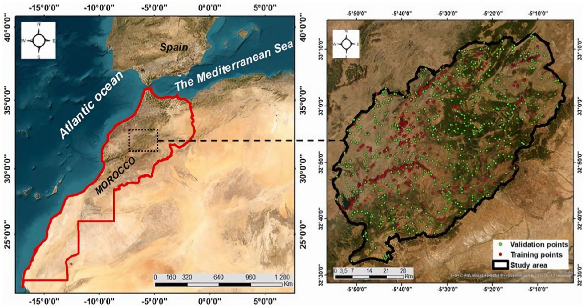
Figure 1. Location of the study area.

The high Oum Er Rbia watershed is characterized by two main tributaries, namely Oued Chbouka, and Oued Srou, with which the confluence at the Ahmed El Hansali Dam. This watershed is characterized by various land uses, involving forests in the Middle Atlas Mountains. The predominant tree species are the evergreen oak and cedar. The climate of the Oum Er Rbia watershed is arid to semi-arid, with rainfall typically concentrated within a few days each month. Precipitation is irregularly distributed, occurring mainly between October to November and April to May, with a peak in December, whereas July and August are nearly dry. The temperature ranges from nearly 0°C in the winter to a high-temperature value in the summer. Consequently, we differentiate two seasons, wet and dry seasons, and surrounding areas demonstrated irregular spatiotemporal rainfall (Karroum et al., 2019).

2.2 Flood inventory

To accurately predict flood-prone areas, it is essential to survey previously flooded regions and identify flood-prone areas within the high Oum Er Rbia watershed. For this purpose, we utilized Google Earth Engine (GEE). To investigate water bodies in the study area, we employed the Normalized Difference Flood Index (NDFI), a method leveraging Sentinel-2 MSI (Multispectral Instrument) Level-2A imagery acquired between 1 January 2019 and 1 January 2022. The Sentinel-2 MSI has a short revisit time of every 5 days at mid-latitudes and every 10 days at the equator (Tarpanelli et al., 2022). This index effectively delineates water features and enhances their visibility in remotely sensed images. It exploits the differential absorption of light by water and other features, allowing for the identification and mapping of water bodies. NDFI is particularly useful in assessing changes in the surface over time. The NDFI is calculated using red (RED) and shortwave infrared 2 (SWIR2) bands (Boschetti et al., 2014). The first step in the delineation of water bodies in GEE is the importation of Sentinel-2 imagery; then, we masked the clouds to indicate a clear condition, and then, we calculated the NDFI using the following equation:

$\mathit{NDFI}=\frac{\mathit{Red}-\mathit{SWIR}2}{\mathit{Red}+\mathit{SWIR}2}$

The specific threshold value was used to distinguish between flood and non-flooded areas using the NDFI can vary based on the region, and the specific characteristics of the landscape. NDFI values typically less than ‘0’ indicate the presence of water, while NDFI values greater than ‘0’ indicate non-water. The image thresholding process generates a binary map that distinguishes flooded and non-flooded areas through visual inspection. Flood-prone areas have a categorical label of “1,” and non-flooded areas were represented by the class value of “0” using binary maps with a specific cutoff thresholding. Therefore, we prepared a flood inventory map, 537 observed points were selected from Sentinel-2. Data are typically divided into two categories: training and testing. Our literature review revealed that approximately 70% of random subsets were selected for training and calibration, with 30% for validation. The methodological flowchart followed in this study is shown in Figure 2.

Figure 2

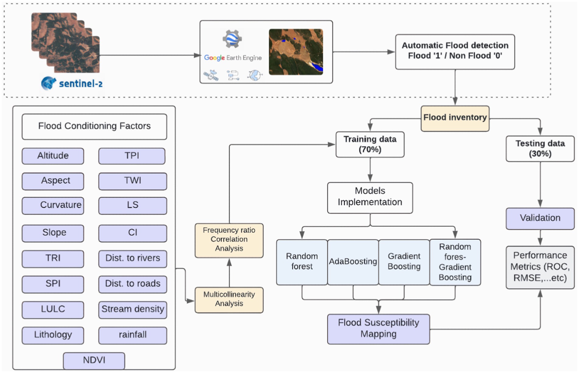
Figure 2. Flowchart of methodology.

2.3 Conditioning factors

Floods are caused by various factors including topography, climate, vegetation, geology, and human activity. This study aimed to map vulnerability to flooding by examining key factors that influence flood occurrence. These factors are displayed in Figures 3–5.

Figure 3

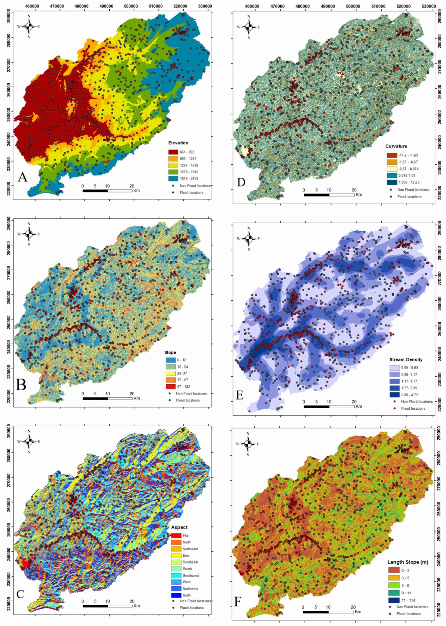
Figure 3. Conditioning factors (A) Elevation; (B) slope; (C) aspect; (D) stream density; (E) slope; (F) length slope.

Figure 4

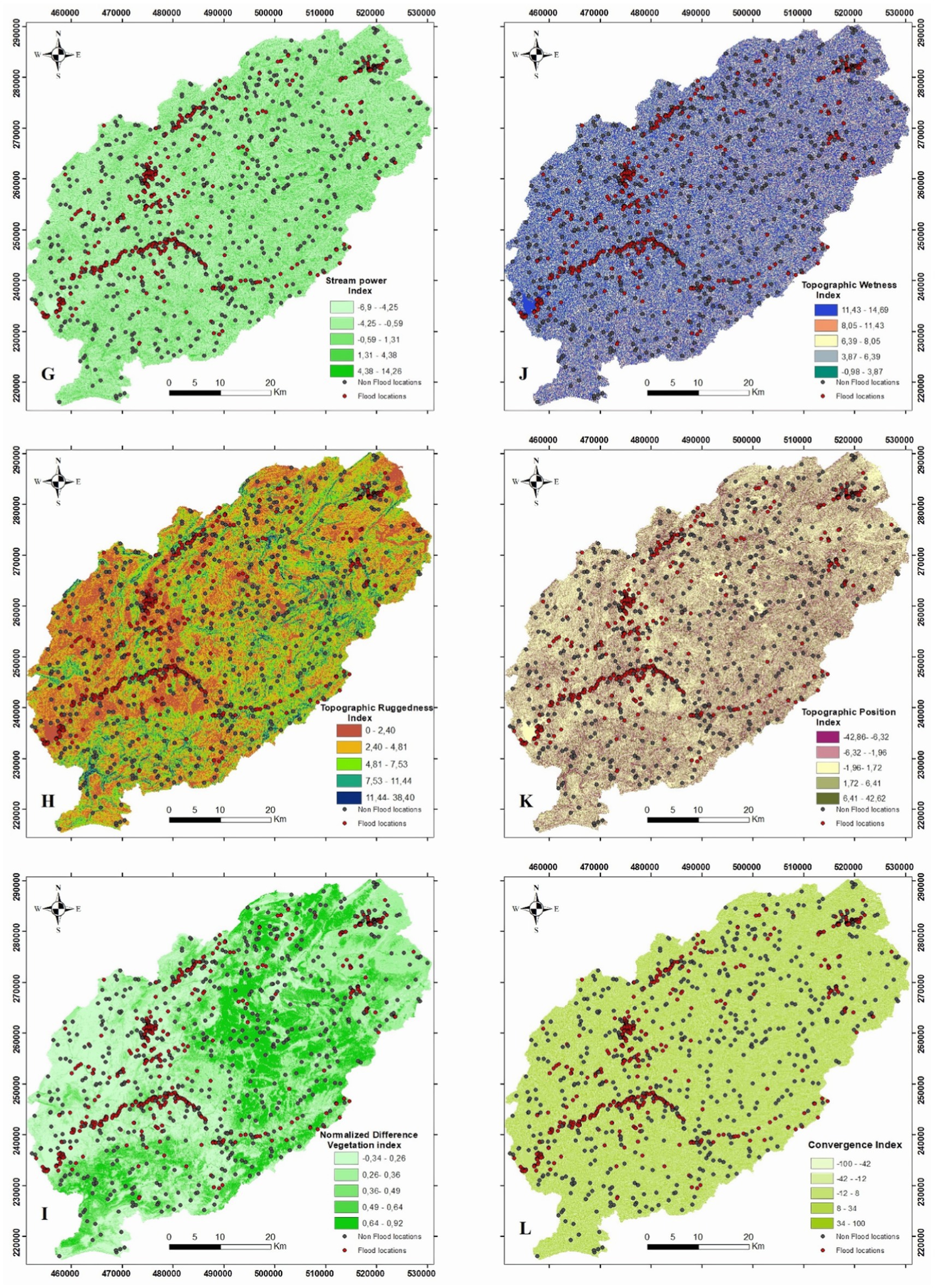
Figure 4. Conditioning factors (G) SPI; (H) TWI; (I) TRI; (J) TPI; (K) NDVI; (L) CI.

Figure 5

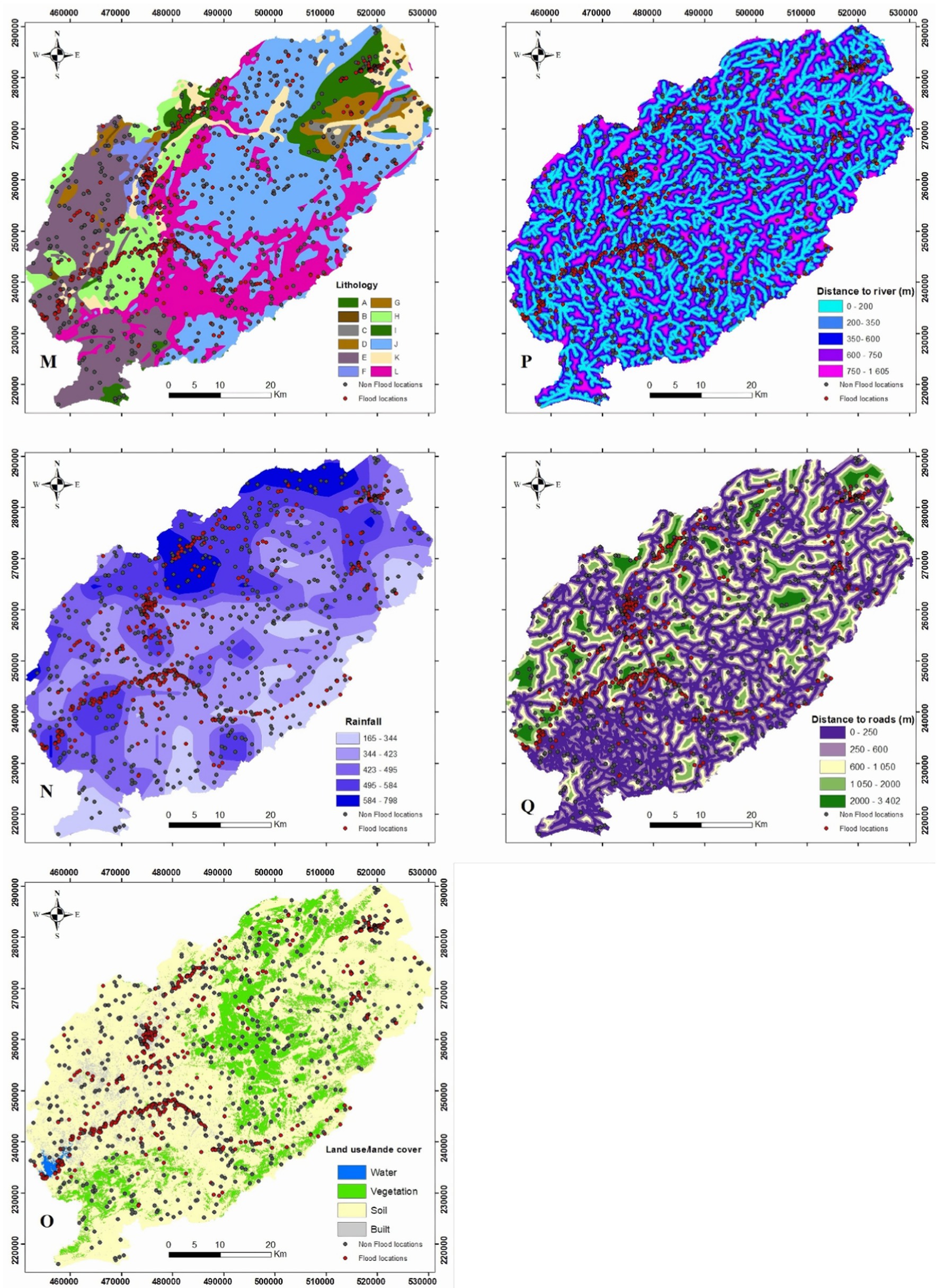
Figure 5. (M) Lithology; (N) rainfall; (P) distance from river; (Q) distance from roads; (O) LULC.

Topography significantly influences the behavior of water both before and during floods. Elevation directly affects flooding risk (Aydin and Iban, 2023; Chowdhuri et al., 2020) as it controls the natural flow of water. Higher elevations have better surface drainage, making them less prone to flooding, while low-elevation areas are more vulnerable. Slope is a significant factor when modeling floods, it influences the direction and speed of the flow of water. Slope relates to the steepness of the land surface. In general, higher slopes are related to more rapid water flow and a higher probability of erosion, whereas flat areas could be more susceptible to slower accumulation of water. Furthermore, the impact of slope on floods varies according to several factors such as the nature of the soil and land use (Al-Kindi and Alabri, 2024). The aspect affects the hydrological parameters, and according to Choubin et al. (2019), there is an indirect relationship between flood and aspect. When an aspect receives a lower sunlight intensity indicating more soil moisture, humid soil will probably raise runoff and increase the risk of flooding. This factor affects rainfall intensity and contributes to the analysis of flood exposure (Yousefi et al., 2020b). Curvature is important in flood hazard modeling; it influences the water flow and the amount of erosion during floods. This refers to the level to which the land surface is convex or concave (Al-Kindi and Alabri, 2024; Chapi et al., 2017). The Topographic Ruggedness Index (TRI) is used to account for local topography when determining flood conditions. Floods are negatively correlated with TRI values, with higher TRI values linked to fewer floods and lower TRI values associated with more floods. The Topographic Wetness Index (TWI) was first proposed by Kirkby (1975) for hydrological modeling in mountains and hilly terrain. TWI indicates the degree of geotechnical wetness and can be used to determine areas susceptible to flooding (Seleem et al., 2022). The Stream Power Index (SPI) measures the potential of erosion. We calculated SPI using the slope, hydraulic radius of a stream, and drainage density. The TWI calculation is defined as Equation 1, whereas SPI is Equation 2, with As representing the catchment area and $\beta$representing the slope gradient in degrees.

$\begin{array}{ll}TWI=\frac{ln{A}_s}{tan\beta }& (1)\end{array}$

$\begin{array}{ll}SPI=A_s\times tan\beta & (2)\end{array}$

The Topographic Position Index (TPI) was calculated using Digital Elevation Model data. The TPI indicated the altitude difference between neighboring and focus cells in DEM. Positive TPI values indicate ridges, whereas negative TPI values represent valleys. TPI values near zero indicate flat areas or areas with constant slope. The Convergence Index represents a significant flood conditioning factor. It calculates an index of convergence for overland by considering the characteristics of surrounding cells. The Convergence Index has negative values for convergent areas and positive values for divergent flow conditions (Kocsis et al., 2022).

Lithology has a crucial role in regulating drainage basin hydrology and sediment protection. The areas with high-resistant rock and permeable subsoil have lower drainage density. The map was created by digitizing the geological map of Morocco (1/1,000,000 scale). The lithology of the study area presents 11 categories or formations: The Jurassic limestone and dolomite cover 41% of the basin in the Middle Atlas, specifically in the Causse area. The remaining 21% of the lithology is made up of magmatic rock, predominantly basalt. The Triassic formation formed an impermeable level. Carboniferous schist accounts for 12% of the area and is primarily found in the west of the basin.

Land use land cover (LULC) has a significant role in flooding, which influences direct as well as indirect impact on sediment transportation and surface runoff. The Normalized Difference Vegetation Index (NDVI) has a negative relationship with flooding, with greater NDVI values indicating a lower probability of flooding and lower NDVI values indicating a higher probability of flooding (Khosravi et al., 2019). Using equation NDVI is calculated as follows (Equation 3):

$\begin{array}{ll}\mathit{NDVI}=\frac{NIR-\mathit{Red}}{NIR+\mathit{Red}}& (3)\end{array}$

Where NIR refers to the near-infrared band and Red represents the red band.

The distance to river has been regarded as an important causative factor. The area closest to the streams is particularly vulnerable to normal floods and flash floods within the river basin because water comes from high elevations and accumulates at lower levels. Flooding hazards increase as the distance to the river decreases, and inversely (Pham et al., 2020). Distance from roads is an anthropogenic factor in analyzing flood-prone areas. Roads decrease the water infiltration process. Consequently, areas with an extensive network of roads are flooded, which causes floods (Osman and Das, 2023).

The rainfall is an important factor in this research study, it triggers overflow, which can lead to floods. Flash floods are often related to brief and intense rainstorms (Bui et al., 2019; Osman and Das, 2023). Stream density is an important factor in determining flood occurrences. Higher stream density in a region increases the risk of flash flooding during rainstorms (Mitra and Das, 2023). Table 1 displays the class intervals and corresponding frequency ratios. Machine learning classifiers were trained and validated using a data frame containing pixel values from each causative factor (Table 2).

Table 1

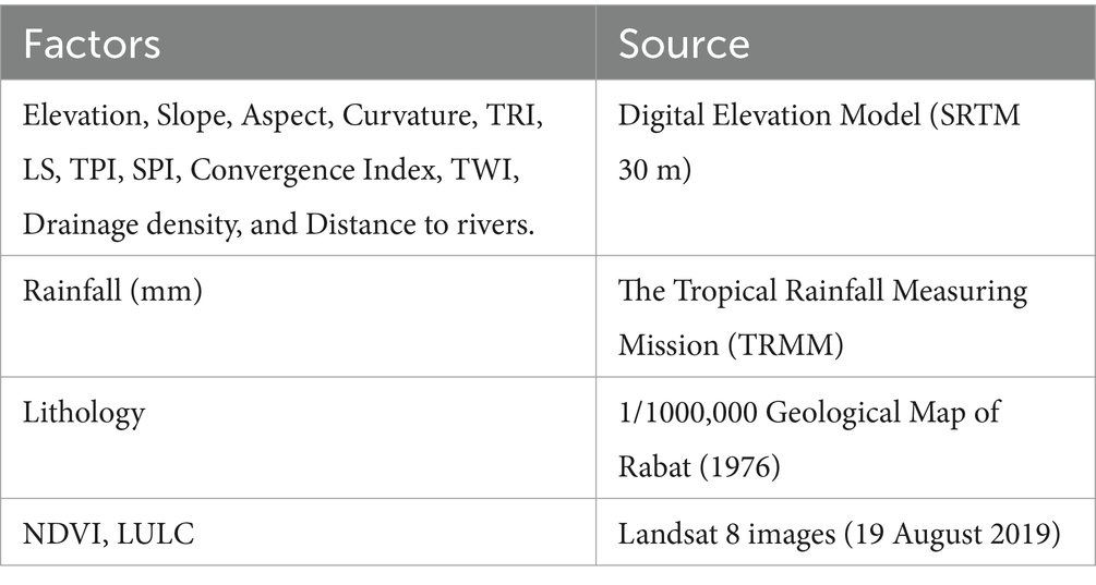
Table 1. Data sources employed in this study.

Table 2

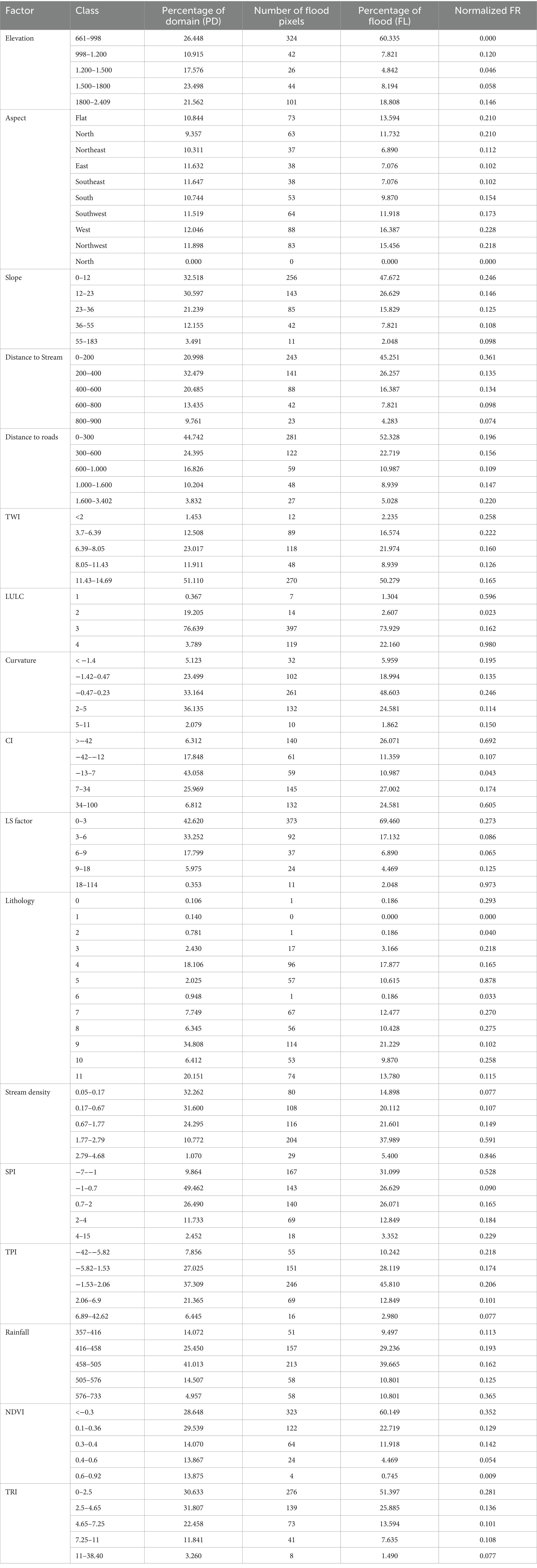
Table 2. Spatial relations between locations and conditioning factors of floods.

2.4 Analysis of conditioning factors

Several factors influence the occurrence of floods, including hydrological, topographic, geological, and anthropogenic factors. A total of 17 variables were considered in this study (Figures 3, 4). The multicollinearity test was carried out on all included conditioning factors.

2.4.1 Collinearity test

Multilinearity (or collinearity) is an analytical technique used in multivariate linear analyses that occurs when multiple predictor variables are related or interrelated (Yariyan et al., 2020). In such research, it is essential to select an approach that may forecast the influence of variables independently (Yousefi et al., 2020a). This study used the variance inflation factor (VIF) to investigate the linearity of flood conditioning factors. If the VIF is greater than 5, the conditioning factors have a linear relationship. The VIF is defined in Equation 4:

$\begin{array}{ll}VI{F}_j=\frac{1}{1-R_j^2}& (4)\end{array}$

Where $R_j^2$ is the coefficient of determination of the regression model and j is the independent variable.

2.5 Spatial analysis of flood susceptibility

2.5.1 Spatial correlation

The frequency ratio method is a statistical approach that can be employed as a basic technique to estimate the probable relationship between the independent factors (causative factors) and dependent variables (flood locations). It contains several categorized maps. This approach is used for mapping flood vulnerability (Yariyan et al., 2020). The frequency ratio technique depends on the observed relationship between flood occurrences and the attributed factors (Sarkar and Mondal, 2019). Equation 5 is employed to calculate FR:

$\begin{array}{ll}FR=\frac{\mathit{Pourcentage}\mathit{of}\mathit{flood}\mathit{location}\left(\mathit{PL}\right)}{\mathit{Pourcentage}\mathit{of}\mathit{pixel}\mathit{of}\mathit{each}\mathit{factor}\left(PD\right)}& (5)\end{array}$

The FR obtained are normalized using Equation 6:

$\begin{array}{ll}F{R}_{\mathit{Normalized}}=\left(\frac{FR-min\left(FR\right)}{max\left(FR\right)-min\left(FR\right)}\right)\ast \left(0.99-0.01\right)+0.01& (6)\end{array}$

2.5.2 Random forest

The random forest model is a highly efficient combination of trees of prediction suggested by Breiman (2001). It is an approach to learning predictions by combining several decision trees. A random subset of feature training data is used to build each decision tree, and for regression problems, the average prediction of each tree is calculated based on the majority of votes for classification. The RF is effective for analyzing ordered associations and non-linearities in large datasets. As a result, the RF method assists in predicting new data samples more accurately. The RF mean square error is expressed as Equation 7:

$\begin{array}{ll}\epsilon ={\left({\vartheta }_{\mathit{observed}}-{\vartheta }_{\mathit{predicted}}\right)}^2& (7)\end{array}$

In this equation, ε represents the algorithm’s mean square error, ${\vartheta }_{\mathit{observed}}$ represents the observed data variables, and ${\vartheta }_{\mathit{predicted}}$ represents the result variables.

The average prediction from trees is determined using Equation 8:

$\begin{array}{ll}S=\frac{1}{K}\sum K^{th}{\vartheta }_{\mathit{predicted}}& (8)\end{array}$

where S represents the random forest prediction, and K applies to each individual tree in the forest.

2.5.3 AdaBoost

AdaBoost (Adaptive Boosting) is a classifier algorithm developed by Freund and Schapire (1997). It is mainly used for classification and the based learner is usually a decision tree with only one level, also called a stump. It improves classification in machine learning. The fj(x) weak classifier generates a Boolean expression (flood or non-flood) and follows a learning sequence. Following each round, samples are reweighted to identify misclassified samples from the previous round. When a specific threshold is found, the sequence ends and a weighted set of weak classifiers produces a stronger classifier. The weakest classifier loses weight when it provides an incorrect class. Excellent classifiers use larger weights. Consequently, an adaptive learning sequence is implemented, and the classification is boosted.

The weights (w₁……w_n) are started with $Wi=\{\frac{1}{m}\mathit{or}\frac{1}{l}$ . The number of flood and non-flood samples are denoted by m and l, respectively. Weights have been normalized to ${\displaystyle \sum }_n^{1}wi=1$ . To train a weak classifier ( $fj\left(x\right)=\left\{1,0\right\}$ ) with labeled classes for each sample j, the training error is calculated in Equation 9:

$\begin{array}{ll}{\epsilon }_j={\displaystyle \sum }_1^{n}wi|fj\left(x\right)-yi|& (9)\end{array}$

The weak classifier f_j (x) with the smallest error in training (𝜀_t) is chosen and assigned an alpha value based on the training error.

$\alpha =log\frac{1}{{\beta }_t}$ where ${\beta }_t=\frac{{\epsilon }_t}{1-{\epsilon }_{t.}}$

To update the weight of appropriately categorized samples, multiply them by 𝛽_t.Therefore, the final ensemble classifier for a given sample is represented by Equation 10:

$\begin{array}{ll}C\left(x\right)={\displaystyle \sum }_1^t{\alpha }_t{f}_t\left(x\right)& (10)\end{array}$

2.5.4 Gradient boosting

Gradient boosting is an algorithm of machine learning algorithms introduced by Friedman (2001). Gradient boosting combines insufficient learning models to form a strong predictive model and is typically carried out using decision trees. Gradient boosting and AdaBoost classifiers use multiple classifiers and average their performance to determine the best one. The GB algorithm is more resistant to outliers as it uses a differentiable loss function for boosting.

2.5.5 Performance assessment

The modeling methodology involved reclassifying continuous variables among causative factors into five categories based on expert knowledge and statistical analysis, using the natural break classification method with GIS tools. It is important to highlight that numerical variables were created from the category variables such as lithology, aspect, and land use/cover. All conditioning factors were converted to raster format 30 × 30 m cell sizes and normalized from 0 to 1 in the following ways so that they could be utilized as input data in the hybrid models.

$X_{\mathit{normalized}}=\frac{X-X_{\text{min}}}{X_{\text{max}}-X_{\text{min}}}$

In this dataset, X represents the original input, X _norm is the normalized input, and X _min and X _max denote the minimum and maximum values of the input ranges. CSV files were generated for Python program modeling using the “Extract values from points” function in the spatial Analyst Toolbox of ArcGIS software (version 10.5).

The flood-predicting dataset was created by combining the flood inventory map with the flood conditioning parameters. These resulting factors, while the final column contains the flood inventory map, where 0 indicates non-flood areas and 1 denotes flooded areas. The number of rows in the flood dataset corresponds to the number of data points or locations used for analysis. Typically, the dataset [1,074 locations (including 537 flood points and 537 randomly flood points) *17 features] is divided into two subsets: 70% for training and 30% for validation. This split can be accomplished with a variety of libraries and programming languages. The scikit-learn library in the Python console was utilized in the current investigation. The flood prediction dataset was analyzed and extracted using a GIS environment.

2.5.6 Model performance metrics

Validation of results is an important step for assessing the accuracy of flood susceptibility models. To evaluate the prediction of the model, it is important to compare both learning and validation datasets (Khosravi et al., 2018). In the current study, we evaluated various validation metrics. The receiver operating characteristic (ROC) curve serves as a graphical representation that displays the true positive rate on the y-axis and the cumulative false positive rate on the x-axis. Additionally, we calculated the area under the ROC curve to assess the model’s performance and evaluated its precision. Finally, the area under the curve was determined using the ROC curve, and the precision of the model was evaluated. The ROC curve is the most widely used technique for assessing flood risk. AUC was used in a number of studies to assess a technique classification performance. An AUC-ROC closer to 1 indicates better model performance, whereas an AUC of 0.5 or lower suggests poor classification ability.

Other quantitative metrics, such as accuracy, sensitivity, specificity, kappa, RMSE, and F1-score, were utilized to assess the model’s performance and evaluate its capacity for classification in relation to other models in the literature. Equation 11 defines accuracy as the ratio of correctly categorized data to total observations, whereas the sensitivity is the proportion of flood pixels that are correctly classified as flood occurrence (Equation 12), while the specificity is the proportion of non-flood pixels that are correctly classified as non-flood (Equation 13). The F1-score represents the weighted average of recall and precision (Equation 14). Kappa is a statistical measure used to evaluate the accuracy and reliability of flood susceptibility models by comparing predicted flood-prone areas with observed data (Equation 15).

$\begin{array}{ll}\mathit{Accuracy}=\frac{TP+TN}{TP+TN+FP+FM}& (11)\end{array}$

$\begin{array}{ll}\mathit{Sensitivity}=\frac{TP}{TP+FN}& (12)\end{array}$

$\begin{array}{ll}\mathit{Specificity}=\frac{TP}{FP+FN}& (13)\end{array}$

$\begin{array}{ll}F1-\mathit{score}=\frac{2TP}{2TP+FP+FN}& (14)\end{array}$

$\begin{array}{ll}\mathit{Kappa}=\frac{{{\displaystyle \sum }}_1^m{\left(\rho i-\sigma i\right)}^2}{m}& (15)\end{array}$

When P and N denote the presence and absence of flooding, TP is the true positive, TN is the true negative, FP is the false positive, and FN is the false negative.

RMSE refers to the difference between simulated and measured values in a model. This index is widely used to evaluate maps that are susceptible to flash floods (Pham et al., 2020). the ability of the model to predict outcomes is improved with decreasing RMSE values. The formula for calculating RMSE is calculated as follows (Equation 16):

$\begin{array}{ll}\mathit{RMSE}=\sqrt{\frac{1}{N}{\displaystyle \sum }_{i=1}^L\left(X_{\mathit{model}}-X_{\mathit{act}}\right)}& (16)\end{array}$

where X _model is the estimated value from the FS model, X _actual is the observed value, and N is the total number of samples in the learning or testing phase.

3 Results

3.1 Multicollinearity analysis

For analyzing multicollinearity, we used VIF and TOL to identify the most significant factors and remove unnecessary causative factors that can negatively impact the performance of the models. Tolerance (TOL) is a measure used in multicollinearity analysis to assess the degree of multicollinearity among predictor variables in a regression model. It is calculated as the reciprocal of the variance inflation factor (VIF); specifically, TOL is defined as:

$TOL=\frac{1}{VIF}$

$TOL=1-R^2$

Multicollinearity tests showed the highest VIF value of 3.09 and the lowest TOL value of 0.32 (Table 3). No conditional factor can be called collinear because it has a TOL of less than 1 and a VIF also lower than 5. Additionally, a correlation matrix was used to assess the redundancy of conditioning factors (Figure 6).

Table 3

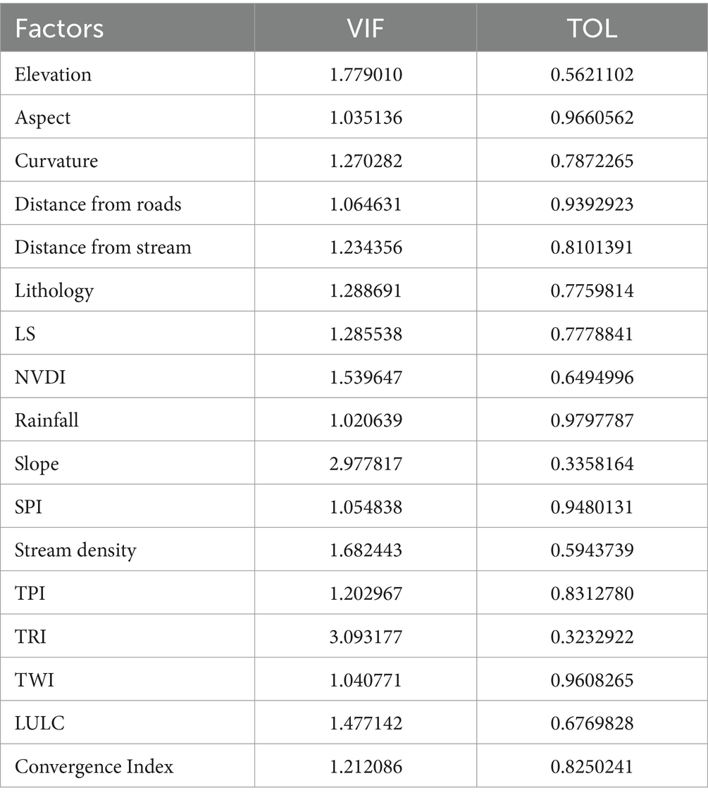
Table 3. Multicollinearity analysis.

Figure 6

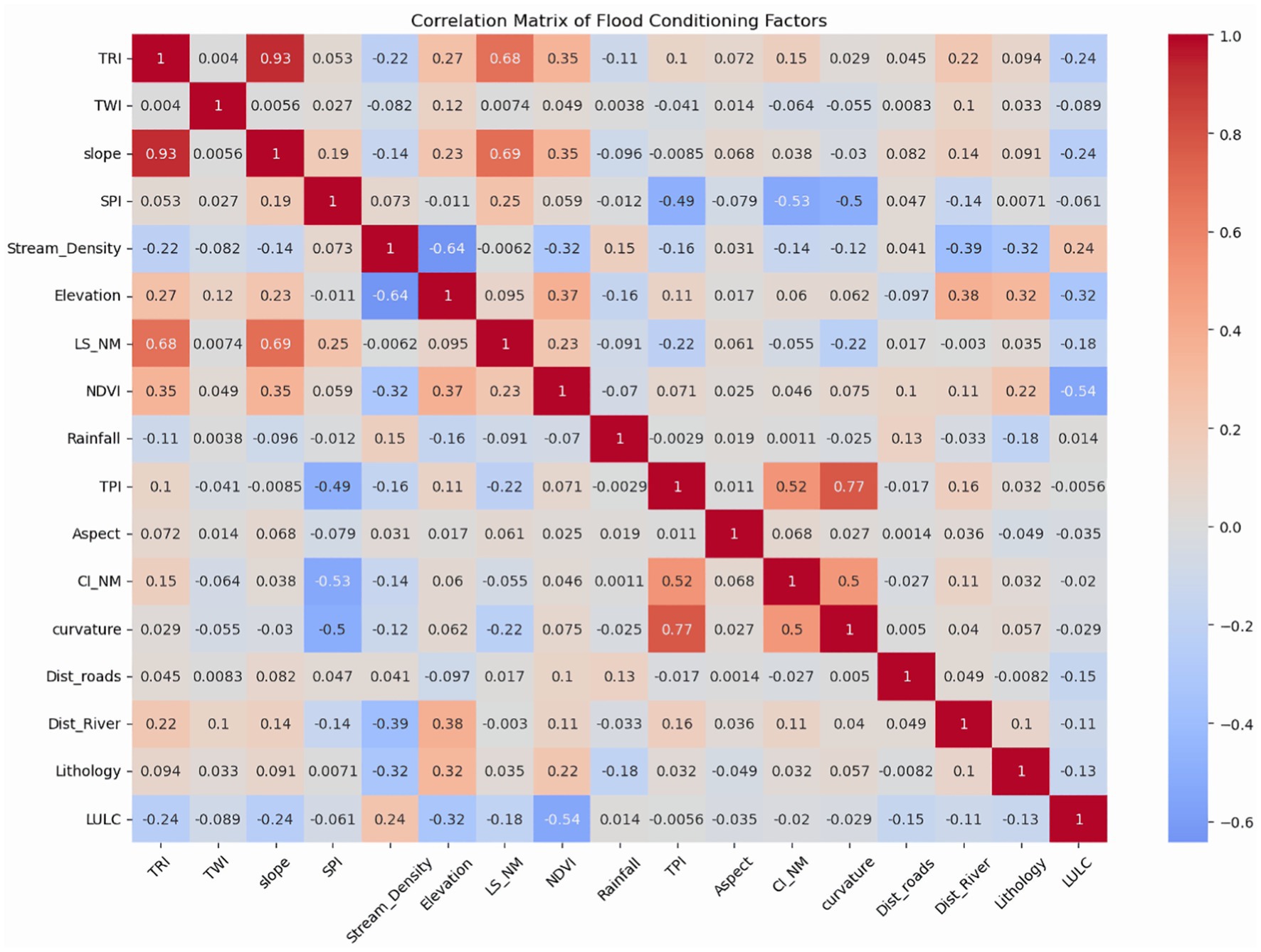
Figure 6. Correlation matrix of flood conditioning factors.

3.2 Spatial correlation using FR analysis

In this study, the frequency ratio (FR) approach was used to analyze the spatial correlation between variable categories and the flood locations. Each variable class was assigned an appropriate weight (Sarkar and Mondal, 2019). The results revealed that the factor class with the highest correlation is the built-up class of LULC, showing the maximum frequency ratio (FR) value of 5.84. This is followed by the LS factor (FR = 5.80) and the lithology class 5 (FR = 5.25). Other high FR values include stream density (FR = 5.04), convergence index (FR = 4.13), SPI (FR = 3.15), elevation (FR = 2,28), and rainfall (FR = 2,17).

3.3 Flood susceptibility mapping

The four models were trained on 70% of the training dataset and tested on 30% of the validating dataset. The predicted. The predicted FSMs were categorized into five classes: very high, high very, moderate, low, and very low. The performance of the model was evaluated using the ROC–AUC curve. The models were trained, validated, and evaluated using a Python environment.

The flood susceptibility maps produced by machine learning models are classified from 0 to 1 on raster maps. Each pixel was assigned a value indicating its vulnerability to flooding. Specifically, a higher value on the scale demonstrates increased susceptibility. Lower values prove lower susceptibility categories (see Table 4 and Figure 7). These classes display the following proportions for the random forest model: 22,3, 28, 25, 16, and 7%. Similarly, gradient boosting was estimated as 20, 22, 21, 16, and 11%, respectively. The flood prediction classes of AdaB were 18, 22, 30, 23, and 5%, while RF-GB estimated 18, 52, 29, and 1% for the susceptibility: very high, high, moderate, low, and very low.

Table 4

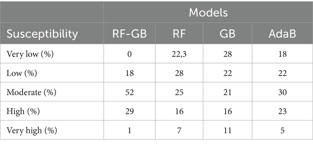
Table 4. Percentage of flood susceptibility.

Figure 7

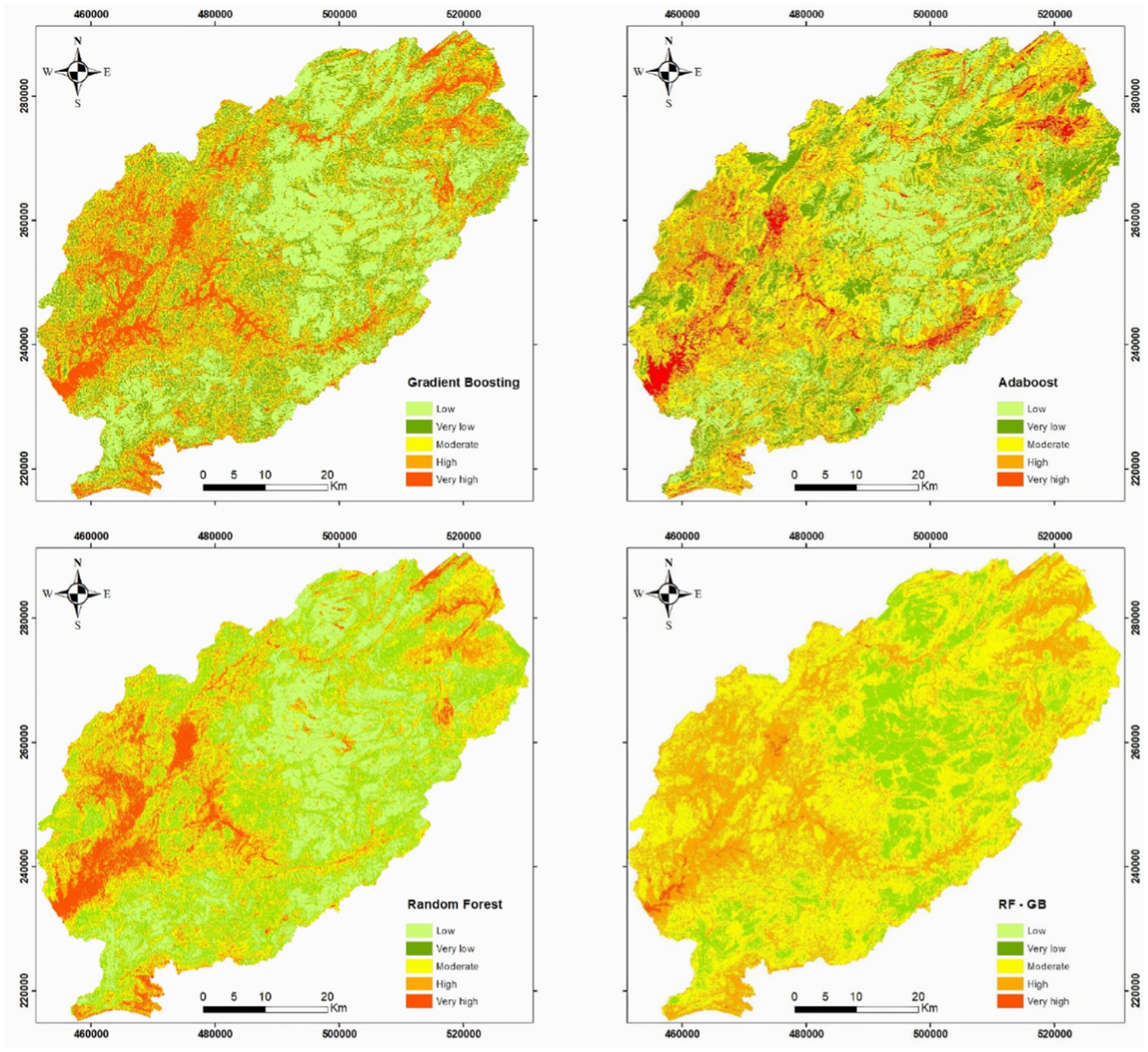
Figure 7. Flood susceptibility mapping developed using machine learning models: (a) gradient boosting; (b) AdaBoost; (c) random forest; (d) random forest–gradient boosting.

Flood-prone areas in the Oum Er Rbia watershed are primarily located around the dam of Ahmed El Hansali, along the Serrou River and in Khenifra City. Flood-prone areas feature varying slopes between high and low terrains, facilitating water accumulation during storms. The slope promotes bank undercutting allowing for easy flow of water. Geologically flood areas in the basin are primarily composed of schist and conglomeratic clay and sand deposits of Trias. The absence of vegetation in these zones also contributes to flooding. In contrast, the high area study is a non-floodable zone characterized by cedar and oak forest, which prevents prolonged flooding.

3.4 Evaluating the performance of ML algorithm

The analysis of the ROC curve indicates that the random forest model was selected as the most effective model in this study, with an average AUC value of 0.98, followed by the RF-GB model scoring an average value of 0.96, then the GB model with the AUC value of 0.95. The last model AdaBoost had an average AUC value of 0.83 as shown in Figure 8. As a result, the random forest proved to be the most effective model in forecasting flood-prone areas. The figure shows the RF, RF-GB, GB, and AdaB algorithms.

Figure 8

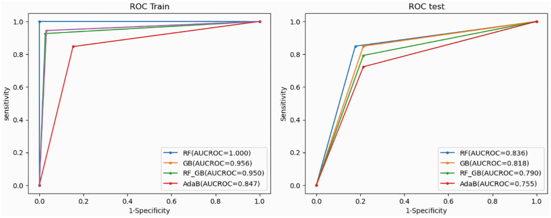
Figure 8. Validation of models using ROC curves and AUC.

Additionally, many statistical parameters were employed, including accuracy, sensitivity, specificity, F1-score, RMSE, and kappa. The accuracy values in RF, RF-GB, GB, and AdaB for the training datasets are as follows: 1, 0.96, 0.95, and 0.84, respectively. For the validation datasets, the accuracy values are:1, 0.79, 0.82, and 0.75 respectively. The sensitivity values of the training datasets in RF, RF-GB, GB, and AdaB are as follows: 1, 0.95, 0.94, and 0.84, respectively. For validation, the datasets are as follows: 0.83, 0.80, 0.84, and 0.72. Regarding training datasets, the specificity values in RF, RF-GB, GB, and AdaB are as follows: 1, 0.80, 0.84, and 0.72, respectively. The values of specificity for training datasets are as follows: 0.83, 0.80, 0.84, and 0.72. The F1-score values for the training datasets are as follows: 1, 0.96, 0.95, and 0.84, respectively. When considering validation datasets in RF, RF-GB, GB, and AdaB, the F1 scores are as follows: 0.83, 0.79, 0.82, and 0.74, respectively. In RF, RF-GB, GB, and AdaB, the RMSE values for training datasets are as follows: 1, 0.18, 0.20, and 0.39, respectively. The RMSE values in RF, RF-GB, GB, and AdaB, for the validation datasets are as follows: 0.40, 0.44, 0.42, and 0.39, respectively. The values of kappa values for the training datasets in RF, RF-GB, GB, and AdaB are as follows: 1, 0.92, 0.91, and 0.69, respectively. When considering validation datasets, the kappa values in RF, RF-GB, GB, and AdaB are as follows: 0.67, 0.59, 0.65, and 0.51 (Table 5), respectively.

Table 5

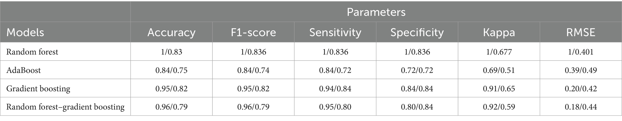
Table 5. The performance models using the training/testing datasets.

3.5 Model explainability

SHapley Additive Explanations, commonly known as SHAP, are employed for explaining the output of machine learning models. SHAP is a feature importance method that helps explain the role of conditioning factors in assessing flood susceptibility (Aydin and Iban, 2023).

This study uses the SHAP techniques to analyze predicted class output from ML models. The SHAP method emphasizes the importance of conditioning factors, their interdependence, and how they impact individual predictions. The SHAP method is currently used in flood susceptibility mapping studies. Aydin and Iban (2023) demonstrate that their best ML can interpreted using the SHAP method. The study identified that slope, elevation, and distance to rivers are the most significant causative factors, with a distinctive contribution. The SHAP assesses whether each factor has a positive or negative impact (Kannangara et al., 2022). To calculate the SHAP value we based on the Python SHAP library (Pradhan et al., 2023).

Figure 9 illustrates SHAP values for input factors, ranked by contribution. The x-axis displays the SHAP value, and the y-axis represents the features (conditioning factors). Each dot represents a sample, and its color indicates the value of a factor, where pink indicates a higher value and blue indicates a lower value. Furthermore, the horizontal position demonstrates whether the conditioning factors impact the prediction positively or negatively. The flood conditioning factors, NDVI, stream density, elevation, and distance to the river are among the top features that have the most significant effect on the random forest model predictions. However, aspect, curvature, and LULC have a smaller impact, with more SHAP values concentrated near zero. The red and blue colors indicate how the feature value affects the prediction. For instance, higher elevation (red) tends to reduce flood risk, while lower elevation (blue) increases the risk. For the AdaBoost model, NDVI, the stream density, distance to a river, and TRI are the most influential features in predicting flood susceptibility, whereas LULC, TWI, and curvature have a lower influence on the model prediction. The AdaBoost model appears to prioritize environmental and topographic factors such as NDVI, stream density, and distance to the river for predicting flood susceptibility. Areas with higher vegetation and elevation tend to have lower flood risks, while proximity to rivers, high stream density, and lower elevation increase susceptibility to flooding. The most influential features in gradient boosting are NDVI, elevation, and distance to the river. However, LULC and length slope have minimal effects on gradient boosting. The gradient boosting model shows that factors related to vegetation (NDVI), topography (elevation), and water bodies (stream density distance to the river) are the most important in determining flood susceptibility.

Figure 9

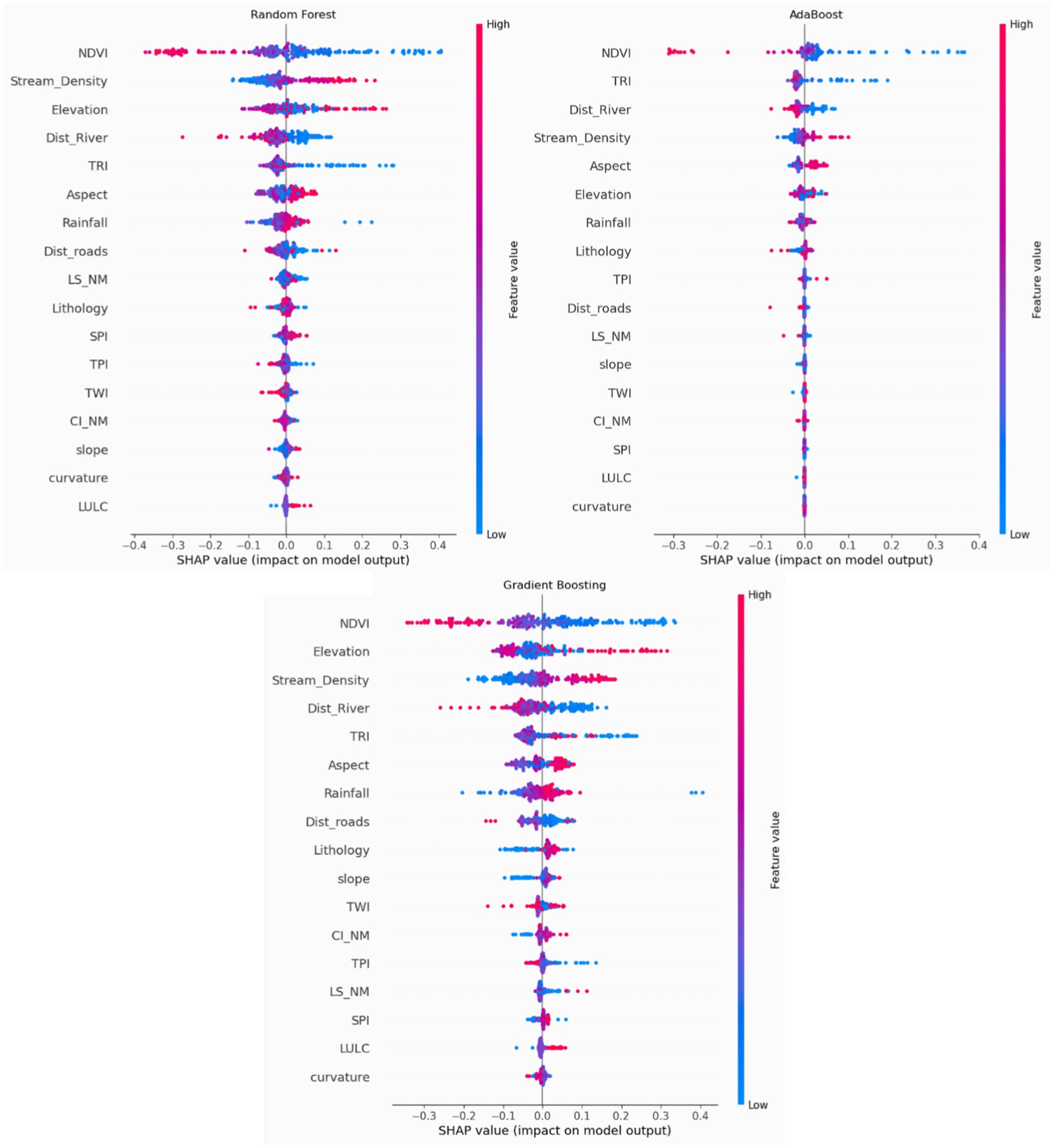
Figure 9. Local explanation of the classifiers (SHAP values).

4 Discussion

4.1 Automation of flood inventories

Flood susceptibility mapping is an essential tool for identifying areas at risk of flooding. To improve both the accuracy and efficiency of this process, the automation of flood inventories using remote sensing data can play a crucial role. The Normalized Difference Flood Index (NDFI) is a useful remote sensing index for flood detection, leveraging the spectral properties of water bodies to identify inundated areas. Typically, derived from multispectral satellite data, practically using the red and shortwave infrared (SWIR2) bands, NDFI offers a reliable method for flood detection. Cloud-based platforms, such as Google Earth Engine (GEE), facilitate the automation of flood inventories, enabling the processing of large datasets in real time, covering extensive areas, and continuously updating flood NDFI to provide faster, more accurate, and cost-effective flood risk assessments, which is particularly important in the context of increasing flood risks due to climate change. Furthermore, authorities can make better-informed decisions and implement targeted flood risk management measures in areas prone to flooding based on these satellite-derived inventories.

4.2 Flood susceptibility mapping

Flood susceptibility mapping is a complex task that involves several uncertainties (Liu et al., 2019). Machine learning (ML) methods can be highly effective in addressing these uncertainties, provided that the flood inventory maps are accurate (Janizadeh et al., 2019). In this study, we employed natural classification techniques within GIS software, assigning five risk categories: lowest, lower, medium, higher, and very high-risk zones.

To improve the flood susceptibility mapping process, we integrated multiple index layers generated by Google Earth Engine (GEE) and applied classification algorithms such as random forest (RF), AdaBoost, gradient boosting (GB), and a combination of random forest and gradient boosting (RF-GB). These models allowed for the creation of a comprehensive flood susceptibility map (Figure 7), identifying regions with varying levels of flood risk.

The study found that the downstream areas of the watershed, characterized by lower elevations, are the most susceptible to flooding. Conversely, higher elevation areas, particularly those covered by cedar forest, exhibit lower flood risk. Regions with dense vegetation, high elevations, and soils with high infiltration capacity are less prone to flooding. The area downstream of the Oum ER Rbia watershed, especially near the Ahmed El Hansali Dam and along Oued Srou near Khenifra City, faces a particularly high flood risk. According to Figure 7, the flood susceptibility map shows that approximately 17% of the study area has the lowest risk, 22% falls under risk, 32% is at moderate risk, 21% is at higher risk, and 6% is at very high risk.

4.3 Method limitations and applicability

While the NDFI is a valuable tool for real-time flood monitoring and post-flood mapping, several limitations must be considered. NDFI is particularly effective for delineating flood extents in urban, agricultural, and rural areas, providing critical data for emergency NDFI data can contribute to climate change studies, helping assess the increasing frequency and intensity of floods in the context of global warming. Furthermore, NDFI can inform policy decisions related to flood mitigation, insurance claims, and environmental protection by protection by providing precise spatial information about flood dynamics.

However, NDFI has notable limitations. Cloud cover during flood events can severely reduce the availability of usable satellite data as floods typically occur during cloud-laden conditions. Dense vegetation can also obscure water bodies, leading to an underestimation of flooded areas. Moreover, in regions with small or fragmented water bodies, low-resolution imagery may result in mixed pixels, where water and land and land are indistinguishable, potentially causing inaccuracies in flood detection.

5 Conclusion

Flood susceptibility mapping using the NDFI combined with machine learning offers a promising strategy for effective flood monitoring and response. By integrating NDFI with advanced machine learning models, such as random forest (RF), gradient boosting (GB), and AdaBoost, more accurate and timely flood susceptibility maps can be produced. This combination enhances the ability to predict flood-prone areas and facilitates proactive flood risk management, ultimately helping reduce flood risks and improve emergency preparedness, protecting both lives and property.

Identifying and controlling the key factors that influence flooding is essential to minimizing its impact. In this study, we applied the NDFI to map flood susceptibility in the Oum Er Rbia watershed, incorporating 537 flood locations and 17 causative factors as input variables. Four machine learning models (RF, GB, AdaBoost, and RF-GB) were flood susceptibility. The random forest (RF) model outperformed the other methods, followed by the RF-GB and GB models, with AdaBoost providing the lowest predictive accuracy.

The SHAP (Shapley Additive Explanations) method was employed for feature selection to assess the relevance of various causative factors. The analysis identified NDVI, stream density, and elevation as the top three factors contributing to flood risk. The SHAP analysis further indicated that areas with low vegetation cover, low stream density, and low elevation are more vulnerable to flooding, reinforcing the importance of these variables in flood susceptibility mapping.

In conclusion, the integration of remote sensing data and machine learning provides a powerful tool for improving flood risk assessments. As remote sensing technologies continue to evolve and machine learning models become more refined, we can expect significant improvements in the accuracy, reliability, and accessibility of flood mapping, offering valuable support for flood risk management in the face of increasing climate-related flood events.

5.1 Recommendations

To enhance the effectiveness of flood management, the following recommendations can be integrated into the existing flood monitoring and response framework:

Local authorities should create detailed, multi-hazard disaster response plans that address not only immediate response but also recovery, long-term resilience, and community engagement.

Authorities should invest in improving and integrating early warning systems for a variety of hazards, from flooding to wildfires, ensuring that these systems reach vulnerable populations.

Local communities should be empowered through training and capacity-building to take proactive measures in disaster risk reduction.

Building codes that prioritize disaster-resilient infrastructures, particularly in disaster-prone areas need to be introduced and enforced.

Local authorities should integrate climate adaptation strategies into their border urban planning and development policies.

Data availability statement

The original contributions presented in the study are included in the article/supplementary material, further inquiries can be directed to the corresponding author.

Author contributions

SH: Conceptualization, Data curation, Formal analysis, Investigation, Methodology, Software, Validation, Visualization, Writing – original draft, Writing – review & editing. SK: Formal analysis, Supervision, Writing – review & editing. KA: Funding acquisition, Resources, Writing – review & editing. AB: Supervision, Writing – review & editing. AE: Supervision, Writing – review & editing. MI: Formal analysis, Funding acquisition, Writing – review & editing. ME: Conceptualization, Validation, Visualization, Software, Writing – review & editing. MC: Formal analysis, Visualization, Writing – review & editing. AK: Funding acquisition, Resources, Writing – review & editing. BM: Funding acquisition, Resources, Writing – review & editing. MN: Supervision, Writing – review & editing, Investigation, Validation.

Funding

The author(s) declare that financial support was received for the research and/or publication of this article. Project number (RSPD2025R546) at King Saud University in Riyadh, Saudi Arabia, and the support of the entire Resilink project team.

Conflict of interest

The authors declare that the research was conducted in the absence of any commercial or financial relationships that could be construed as a potential conflict of interest.

Generative AI statement

The author(s) declare that no Gen AI was used in the creation of this manuscript.

Publisher’s note

All claims expressed in this article are solely those of the authors and do not necessarily represent those of their affiliated organizations, or those of the publisher, the editors and the reviewers. Any product that may be evaluated in this article, or claim that may be made by its manufacturer, is not guaranteed or endorsed by the publisher.

References

Afzal, M. A., Ali, S., Nazeer, A., Khan, M. I., Waqas, M. M., Aslam, R. A., et al. (2022). Flood inundation modeling by integrating HEC–RAS and satellite imagery: a case study of the Indus River Basin. Water 14:2984. doi: 10.3390/w14192984

Crossref Full Text | Google Scholar

Alarifi, S. S., Abdelkareem, M., Abdalla, F., and Alotaibi, M. (2022). Flash flood Hazard mapping using remote sensing and GIS techniques in southwestern Saudi Arabia. Sustain. For. 14:14145. doi: 10.3390/su142114145

Crossref Full Text | Google Scholar

Albertini, C., Gioia, A., Iacobellis, V., and Manfreda, S. (2022). Detection of surface water and floods with multispectral satellites. Remote Sens. 14:6005. doi: 10.3390/rs14236005

Crossref Full Text | Google Scholar

Al-Kindi, K. M., and Alabri, Z. (2024). Investigating the role of the key conditioning factors in flood susceptibility mapping through machine learning approaches. Earth Syst. Environ. 8, 63–81. doi: 10.1007/s41748-023-00369-7

Crossref Full Text | Google Scholar

Aydin, H. E., and Iban, M. C. (2023). Predicting and analyzing flood susceptibility using boosting-based ensemble machine learning algorithms with SHapley additive exPlanations. Nat. Hazards 116, 2957–2991. doi: 10.1007/s11069-022-05793-y

Crossref Full Text | Google Scholar

Boschetti, M., Nutini, F., Manfron, G., Brivio, P. A., and Nelson, A. (2014). Comparative analysis of normalised difference spectral indices derived from MODIS for detecting surface water in flooded Rice cropping systems. PLoS One 9:e88741. doi: 10.1371/journal.pone.0088741

PubMed Abstract | Crossref Full Text | Google Scholar

Breiman, L., (2001). Random Forests. Mach. Learn. 45, 5–32.

Google Scholar

Bui, D. T., Tsangaratos, P., Ngo, P.-T. T., Pham, T. D., and Pham, B. T. (2019). Flash flood susceptibility modeling using an optimized fuzzy rule based feature selection technique and tree based ensemble methods. Sci. Total Environ. 668, 1038–1054. doi: 10.1016/j.scitotenv.2019.02.422

Crossref Full Text | Google Scholar

Chapi, K., Singh, V. P., Shirzadi, A., Shahabi, H., Bui, D. T., Pham, B. T., et al. (2017). A novel hybrid artificial intelligence approach for flood susceptibility assessment. Environ. Model. Softw. 95, 229–245. doi: 10.1016/j.envsoft.2017.06.012

Crossref Full Text | Google Scholar

Choubin, B., Moradi, E., Golshan, M., Adamowski, J., Sajedi-Hosseini, F., and Mosavi, A. (2019). An ensemble prediction of flood susceptibility using multivariate discriminant analysis, classification and regression trees, and support vector machines. Sci. Total Environ. 651, 2087–2096. doi: 10.1016/j.scitotenv.2018.10.064

Crossref Full Text | Google Scholar

Chowdhuri, I., Pal, S. C., and Chakrabortty, R. (2020). Flood susceptibility mapping by ensemble evidential belief function and binomial logistic regression model on river basin of eastern India. Adv. Space Res. 65, 1466–1489. doi: 10.1016/j.asr.2019.12.003

Crossref Full Text | Google Scholar

Dodangeh, E., Choubin, B., Eigdir, A. N., Nabipour, N., Panahi, M., Shamshirband, S., et al. (2020). Integrated machine learning methods with resampling algorithms for flood susceptibility prediction. Sci. Total Environ. 705:135983. doi: 10.1016/j.scitotenv.2019.135983

Crossref Full Text | Google Scholar

Errico, A., Lama, G.F.C., Francalanci, S., Chirico, G.B., Solari, L., and Preti, F., (2019). Validation of global flow resistance models in two experimental drainage channels covered by phragmites australis (common reed).

Google Scholar

Freund, Y., and Schapire, R. E. (1997). A Decision-Theoretic Generalization of On-Line Learning and an Application to Boosting. J. Comput. Syst. Sci. 55, 119–139. doi: 10.1006/jcss.1997.1504

Crossref Full Text | Google Scholar

Friedman, J. H. (2001). Greedy Function Approximation: A Gradient Boosting Machine. The Annals of Statistics, 29, 1189–1232. doi: 10.1214/aos/1013203451

Crossref Full Text | Google Scholar

Goffi, A., Stroppiana, D., Brivio, P. A., Bordogna, G., and Boschetti, M. (2020). Towards an automated approach to map flooded areas from Sentinel-2 MSI data and soft integration of water spectral features. Int. J. Appl. Earth Obs. Geoinf. 84:101951. doi: 10.1016/j.jag.2019.101951

Crossref Full Text | Google Scholar

Hapciuc, O., Romanescu, G., Minea, I., Iosub, M., Enea, A., and Sandu, I., (2016). Flood susceptibility analysis of the cultural heritage in the sucevita catchment (Romania).

Google Scholar

Hitouri, S., Mohajane, M., Lahsaini, M., Ali, S. A., Setargie, T. A., Tripathi, G., et al. (2024). Flood susceptibility mapping using SAR data and machine learning algorithms in a small watershed in northwestern Morocco. Remote Sens. 16:858. doi: 10.3390/rs16050858

Crossref Full Text | Google Scholar

Janizadeh, S., Avand, M., Jaafari, A., Phong, T. V., Bayat, M., Ahmadisharaf, E., et al. (2019). Prediction success of machine learning methods for flash flood susceptibility mapping in the Tafresh watershed, Iran. Sustain. For. 11:5426. doi: 10.3390/su11195426

Crossref Full Text | Google Scholar

Kannangara, K. K. P. M., Zhou, W., Ding, Z., and Hong, Z. (2022). Investigation of feature contribution to shield tunneling-induced settlement using Shapley additive explanations method. J. Rock Mech. Geotech. Eng. 14, 1052–1063. doi: 10.1016/j.jrmge.2022.01.002

Crossref Full Text | Google Scholar

Karroum, L. A., El Baghdadi, M., Barakat, A., Rachid, M., Mohamed, A., Oumenskou, H., et al. (2019). Hydrochemical characteristics and water quality evaluation of the Srou River and its tributaries (middle atlas, Morocco) for drinking and agricultural purposes. Desalination Water Treat. 146, 152–164. doi: 10.5004/dwt.2019.23632

Crossref Full Text | Google Scholar

Khosravi, K., Pham, B. T., Chapi, K., Shirzadi, A., Shahabi, H., Revhaug, I., et al. (2018). A comparative assessment of decision trees algorithms for flash flood susceptibility modeling at Haraz watershed, northern Iran. Sci. Total Environ. 627, 744–755. doi: 10.1016/j.scitotenv.2018.01.266

Crossref Full Text | Google Scholar

Khosravi, K., Shahabi, H., Pham, B. T., Adamowski, J., Shirzadi, A., Pradhan, B., et al. (2019). A comparative assessment of flood susceptibility modeling using multi-criteria decision-making analysis and machine learning methods. J. Hydrol. 573, 311–323. doi: 10.1016/j.jhydrol.2019.03.073

Crossref Full Text | Google Scholar

Kirkby, M. J. (1975). Hydrograph Modelling Strategies. In Progress in Physical and Human Geography, R. F. Peel, M. D. Chisholm, and P. Haggett (Eds.), Heinemann, London, pp. 69–90.

Google Scholar

Kocsis, I., Bilașco, Ș., Irimuș, I.-A., Dohotar, V., Rusu, R., and Roșca, S. (2022). Flash Flood Vulnerability Mapping Based on FFPI Using GIS Spatial Analysis Case Study: Valea Rea Catchment Area, Romania. Sensors 22:3573. doi: 10.3390/s22093573

Crossref Full Text | Google Scholar

Kumar, A., Houze, R. A., Rasmussen, K. L., and Peters-Lidard, C. (2014). Simulation of a flash flooding storm at the steep edge of the Himalayas. J. Hydrometeorol. 15, 212–228. doi: 10.1175/JHM-D-12-0155.1

Crossref Full Text | Google Scholar

Lama, G.F.C., and Chirico, G.B., (2020). Effects of reed beds management on the hydrodynamic behaviour of vegetated open channels.

Google Scholar

Lama, G.F.C., and Crimaldi, M., (2021). Assessing the role of gap fraction on the leaf area index (LAI) estimations of riparian vegetation based on fisheye lenses.

Google Scholar

Liu, W., Carling, P. A., Hu, K., Wang, H., Zhou, Z., Zhou, L., et al. (2019). Outburst floods in China: a review. Earth-Sci. Rev. 197:102895. doi: 10.1016/j.earscirev.2019.102895

Crossref Full Text | Google Scholar

Liu, Y., Xu, Y., Zhao, Y., and Long, Y. (2022). Using SWAT model to assess the impacts of land use and climate changes on flood in the upper Weihe River, China. Water 14:2098. doi: 10.3390/w14132098

Crossref Full Text | Google Scholar

Mangukiya, N. K., and Yadav, S. M. (2022). Integrating 1D and 2D hydrodynamic models for semi-arid river basin flood simulation. Int. J. Hydrol. Sci. Technol. 14:206. doi: 10.1504/IJHST.2022.124549

Crossref Full Text | Google Scholar

Mitra, R., and Das, J. (2023). A comparative assessment of flood susceptibility modelling of GIS-based TOPSIS, VIKOR, and EDAS techniques in the sub-Himalayan foothills region of eastern India. Environ. Sci. Pollut. Res. 30, 16036–16067. doi: 10.1007/s11356-022-23168-5

PubMed Abstract | Crossref Full Text | Google Scholar

Mohammad, L., Bandyopadhyay, J., Sk, R., Mondal, I., Trinh Trong, N., Lama, G. F. C., et al. (2023). Estimation of agricultural burned affected area using NDVI and dNBR satellite-based empirical models. J. Environ. Manag. 343:8226. doi: 10.1016/j.jenvman.2023.118226

Crossref Full Text | Google Scholar

Mukhtar, M. A., Shangguan, D., Ding, Y., Anjum, M. N., Banerjee, A., Butt, A. Q., et al. (2024). Integrated flood risk assessment in Hunza-Nagar, Pakistan: unifying big climate data analytics and multi-criteria decision-making with GIS. Front. Environ. Sci. 12:1337081. doi: 10.3389/fenvs.2024.1337081

Crossref Full Text | Google Scholar

Osman, S. A., and Das, J. (2023). GIS-based flood risk assessment using multi-criteria decision analysis of Shebelle River basin in southern Somalia. SN Appl. Sci. 5:134. doi: 10.1007/s42452-023-05360-5

Crossref Full Text | Google Scholar

Pham, B., Avand, M., Janizadeh, S., Tran, P., Al-Ansari, N., Lanh, H., et al. (2020). GIS based hybrid computational approaches for flash flood susceptibility assessment. Water 12:683. doi: 10.3390/w12030683

Crossref Full Text | Google Scholar

Pirone, D., Cimorelli, L., and Pianese, D. (2024). The effect of flood-mitigation reservoir configuration on peak-discharge reduction during preliminary design. J. Hydrol. Reg. Stud. 52:101676. doi: 10.1016/j.ejrh.2024.101676

Crossref Full Text | Google Scholar

Pradhan, B., Lee, S., Dikshit, A., and Kim, H. (2023). Spatial flood susceptibility mapping using an explainable artificial intelligence (XAI) model. Geosci. Front. 14:101625. doi: 10.1016/j.gsf.2023.101625

Crossref Full Text | Google Scholar

Rahmati, O., Pourghasemi, H.R., and Zeinivand, H., (2016). Flood susceptibility mapping using frequency ratio and weights-of-evidence models in the Golastan Province, Iran. Geocarto Int.

Google Scholar

Sarkar, D., and Mondal, P. (2019). Flood vulnerability mapping using frequency ratio (FR) model: a case study on Kulik river basin, indo-Bangladesh Barind region. Appl Water Sci 10:17. doi: 10.1007/s13201-019-1102-x

Crossref Full Text | Google Scholar

Seleem, O., Ayzel, G., Souza, A., Bronstert, A., and Heistermann, M. (2022). Towards urban flood susceptibility mapping using data-driven models in Berlin, Germany. Geomat. Nat. Hazards Risk 13:2097131. doi: 10.1080/19475705.2022.2097131

Crossref Full Text | Google Scholar

Sepehri, M., Malekinezhad, H., Jahanbakhshi, F., Ildoromi, A. R., Chezgi, J., Ghorbanzadeh, O., et al. (2020). Integration of interval rough AHP and fuzzy logic for assessment of flood prone areas at the regional scale. Acta Geophys. 68, 477–493. doi: 10.1007/s11600-019-00398-9

Crossref Full Text | Google Scholar

Shah, Z., Saraswat, A., Samal, D. R., and Patel, D. (2022). A single interface for rainfall-runoff simulation and flood assessment—a case of new capability of HEC-RAS for flood assessment and management. Arab. J. Geosci. 15:1526. doi: 10.1007/s12517-022-10721-2

Crossref Full Text | Google Scholar

Tarpanelli, A., Mondini, A. C., and Camici, S. (2022). Effectiveness of Sentinel-1 and Sentinel-2 for flood detection assessment in Europe. Nat. Hazards Earth Syst. Sci. 22, 2473–2489. doi: 10.5194/nhess-22-2473-2022

Crossref Full Text | Google Scholar

Tazmul Islam, M., and Meng, Q. (2022). An exploratory study of Sentinel-1 SAR for rapid urban flood mapping on Google earth engine. Int. J. Appl. Earth Obs. Geoinf. 113:103002. doi: 10.1016/j.jag.2022.103002

Crossref Full Text | Google Scholar

Vu, V. T., Nguyen, H. D., Vu, P. L., Ha, M. C., Bui, V. D., Nguyen, T. O., et al. (2023). Predicting land use effects on flood susceptibility using machine learning and remote sensing in coastal Vietnam. Water Pract. Technol. 18, 1543–1555. doi: 10.2166/wpt.2023.088

Crossref Full Text | Google Scholar

Xu, H. (2005). A study on information extraction of water body with the modified normalized difference water index (MNDWI). J. Remote Sens. 589–595. doi: 10.11834/jrs.20050586

Crossref Full Text | Google Scholar

Yariyan, P., Avand, M., Abbaspour, R. A., Torabi Haghighi, A., Costache, R., Ghorbanzadeh, O., et al. (2020). Flood susceptibility mapping using an improved analytic network process with statistical models. Geomat. Nat. Hazards Risk 11, 2282–2314. doi: 10.1080/19475705.2020.1836036

Crossref Full Text | Google Scholar

Yousefi, S., Avand, M., Yariyan, P., Pourghasemi, H. R., Keesstra, S., Tavangar, S., et al. (2020a). A novel GIS-based ensemble technique for rangeland downward trend mapping as an ecological indicator change. Ecol. Indic. 117:106591. doi: 10.1016/j.ecolind.2020.106591

Crossref Full Text | Google Scholar

Yousefi, S., Pourghasemi, H. R., Emami, S. N., Pouyan, S., Eskandari, S., and Tiefenbacher, J. P. (2020b). A machine learning framework for multi-hazards modeling and mapping in a mountainous area. Sci. Rep. 10:12144. doi: 10.1038/s41598-020-69233-2

Crossref Full Text | Google Scholar