Streamflow and sediment simulation in the Song River basin using the SWAT model

This study assesses the performance of the Soil and Water Assessment Tool (SWAT) in simulating streamflow and sediment for the Song River watershed, with a focus on calibration, validation, and sensitivity analysis. Thirteen parameters were selected for calibration, with eight identified as highly sensitive, reflecting key hydrological processes of the area. The model was calibrated for the period 1974–1995 and validated from 1996 to 2004, with additional testing using field data collected in 2022–2023 through Acoustic Doppler Current Profiler (ADCP) measurements. Key model adjustments, such as the baseflow recession constant (ALPHA_BF) and channel roughness coefficient (CH_N2), were set to 0.05 and 0.04, respectively, to capture the area’s groundwater dynamics and channel characteristics. The calibration results indicated a strong fit, with R² values of 0.77, NSE of 0.70, and PBIAS of 17.06, demonstrating good agreement between observed and simulated streamflow. Validation showed slightly lower but acceptable performance, with R² of 0.75 and NSE of 0.68. Further ADCP validation from field data showed R² values of 0.79 and 0.78 for two monitoring sites, confirming the model’s reliability. Sediment yield simulations at site-2 yielded R² values of 0.70 and 0.59 for calibration and validation, with NSE values of 0.53 and 0.52, indicating the model’s capability to simulate both streamflow and sediment accurately. These results demonstrate SWAT’s practical utility for water resource management in similar data-limited regions.

1 Introduction

Accurate estimation of streamflow and sediment generation is crucial for effective water resources management. Hydrological models serve as fundamental tools for simulating these processes and have been extensively utilized for both change detection and attribution in catchment systems (Folton et al., 2015; Hassan et al., 2010; Vandenberghe et al., 2006). Inappropriate application of these models may result in erroneous understanding and suboptimal policy recommendations. Daggupati et al. (2015) assert that the requisite modeling accuracy may vary for different applications, contingent upon the risk associated with actions that follow model implementation (e.g., explanatory, planning and/or regulatory).

Surface water resources, particularly rivers, are essential for sustaining ecosystems, human settlements, and economic activities worldwide (Mishra and Saxena, 2024; Kumar and Sen, 2023). Global warming-induced changes in weather patterns, urban expansion, industrial growth, and agricultural chemical use are transforming water resources (Joseph et al., 2018; Kaur and Sinha, 2019). Numerous areas face freshwater shortages or contamination issues. Hydrological elements such as evaporation, transpiration, soil moisture, and runoff are highly responsive to slight changes in temperature and precipitation (Brutsaert and Parlange, 1998; Seneviratne et al., 2010). Consequently, addressing water resource challenges, including the effects of urban development, alternative management approaches, and future climate variations on streamflow and water quality, necessitates a comprehensive understanding and accurate modeling of Earth surface processes at the catchment level (Kumar and Paramanik, 2020; Iwanaga et al., 2020; Gassman et al., 2014; Koltsida et al., 2023). Examining various components of the hydrological process is necessary to evaluate and quantify sediment and auricular chemical yields (Ghoraba, 2015).

Due to the complexity of hydrological processes, various models have been developed over time to facilitate the comprehension of the hydrological system (Arnold and Allen, 1996; Sahu et al., 2016). These hydrological models are essential tools for evaluating catchment behavior, informing decisions on water resource projects, flood control, pollution management, and numerous other applications (Gupta et al., 2024; Pérez-Sánchez et al., 2019; Kumar and Sen, 2024). Among these, semi-distributed hydrological models can simulate water balance spatially by accounting for various soils, land uses, topographical features, and climate conditions (Rafiei Emam et al., 2017). The semi-distributed hydrologic model SWAT is renowned for providing detailed information on water resources in a river basin and projecting the impact of land use changes and management practices on water quantity and quality (Janjić and Tadić, 2023; Gelete et al., 2023; Narsimlu et al., 2015). Researchers have applied the SWAT model across various regions, from arid and semi-arid to humid and tropical (Nguyen and Kappas, 2015; Samimi, 2020). Schuol et al. (2008) assessed the distribution of blue and green water in Africa; Phuong et al. (2014) utilized SWAT to estimate surface runoff and soil erosion in a small part of Vietnam. Understanding runoff and sediment yield dynamics in watersheds is crucial for effective management, especially in data-scarce regions such as the Western Himalayan area. Jain et al. (2010) employed SWAT to estimate runoff and sediment yield in the Suni to Kasol watershed, achieving satisfactory R² coefficients for both daily and monthly values. Similarly, Agrawal et al. (2011) simulated surface runoff and sediment yield in the Chhokranala watershed, emphasizing the impact of calibrated Manning’s “n” values on sediment yield. Aawar and Khare (2020) utilized the SWAT model to analyze the climate change impact on the streamflow of the Kabul River; Bouslihim et al. (2016) opted for the SWAT model to access the hydrological components of the Sebou watershed (Morocco). The SWAT model can also simulate basin hydrology in terms of both quantity and quality by incorporating agricultural practices, point sources, and non-point sources. Thus, the primary objective of this study is to apply the SWAT model to simulate the hydrological processes and sediment yield in the Song River watershed.

2 Methods

2.1 Study area

The Song River, originating from various small streams in the Dhanolti mountain range and merging with Sahastradhara streams, flows down to the Doon valley basins before eventually joining the Ganga River. Known for its picturesque surroundings, the Song River in Dehradun is particularly renowned for its plentiful natural sulphur springs. These springs emerge from mountain fissures and feed into the main watercourse, enriching the river with sulphur. Visitors flock to immerse themselves in the mineral-rich waters, as sulphur baths are thought to alleviate various health issues, particularly skin conditions. Situated at 30°28′ latitude and 78°8′ longitude, the Song River is vital to the communities of Raiwala, Doiwala, Chiddarwala, and Lacchiwala, serving as their primary water source along its 107 km journey. It converges with the Ganga River at 78° 14′ 54″ longitude and 30° 02′ 02″ latitude, just upstream of Haridwar near the Satyanarayan G&D station maintained by CWC, after passing through the Satyanarayana area (Figure 1).

Figure 1

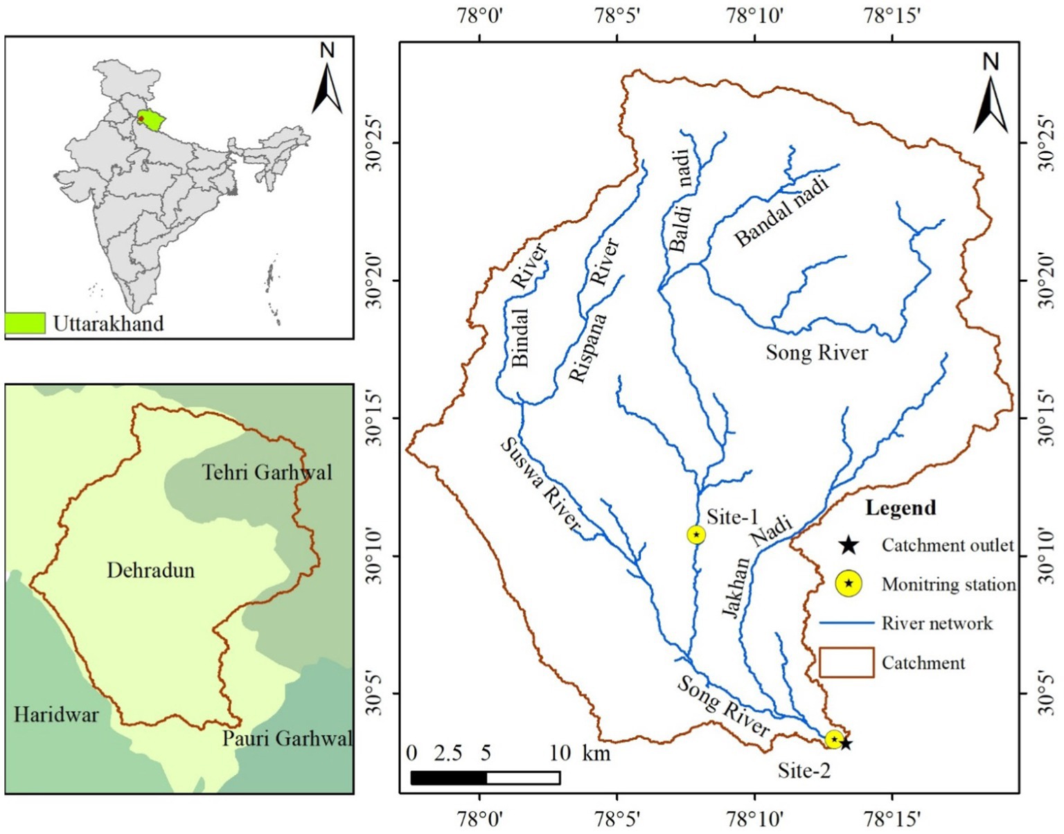
Figure 1. Map of Song River basin, drainage network and selected sites.

A significant tributary of the Song River is the Suswa River, which originates in the clayey depression of the Mussoorie range. It drains the eastern part of Dehradun city and joins the Song River southeast of Doiwala. The catchment area includes two major urban settlements: Dehradun and Doiwala. The Rispana and Bindal, two primary drainage networks, carry municipal sewage from these urban areas and discharge into the Song River via the Suswa River. The region experiences an average annual rainfall of approximately 1,451 mm, with about 1,181 mm (81%) occurring during the monsoon season. Consequently, July and August are the wettest months of the year.

2.2 Model input

2.2.1 Spatial database

Digital Elevation Model (DEM) are critical tools in hydrological modeling as they provide detailed topographical data necessary for analyzing basin characteristics (Figure 3A). DEM are utilized to generate key hydrological parameters, including flow direction, flow accumulation, stream networks, and watershed boundaries. In this study, the FABDEM (Forest and Buildings Removed Copernicus DEM), a state-of-the-art dataset available at a 1 arc-second resolution (approximately 30 m), was employed (Figure 3B). This dataset, freely accessible through the University of Bristol website, offers refined elevation data critical for accurate terrain analysis. Alongside the DEM, Land Use Land Cover (LULC) and soil maps were utilized as essential inputs for hydrological modeling using the SWAT model. The LULC map was developed using Landsat 8 satellite imagery at a 30 m resolution, sourced from the USGS Earth Explorer platform. A supervised classification technique, specifically the Maximum Likelihood Classification method, was applied using ERDAS IMAGINE software to categorize the basin into five land cover classes: water bodies, forest, built-up areas, agricultural land, and riverbed/wasteland. Validation of the LULC map was conducted using ground truth data collected via portable GPS devices during field surveys, revealing that 68% of the catchment is forested and 14% is under agricultural use (Figure 3C).

Figure 2

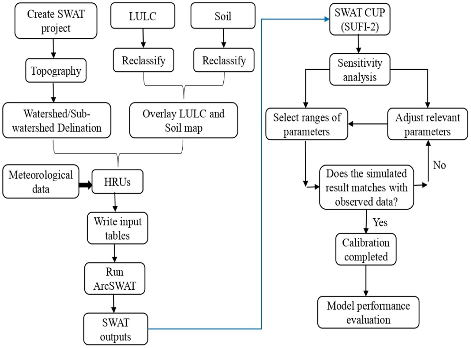
Figure 2. Flow diagram emphasizing the essential elements and processes involved in the hydrological modelling for the study area.

Figure 3

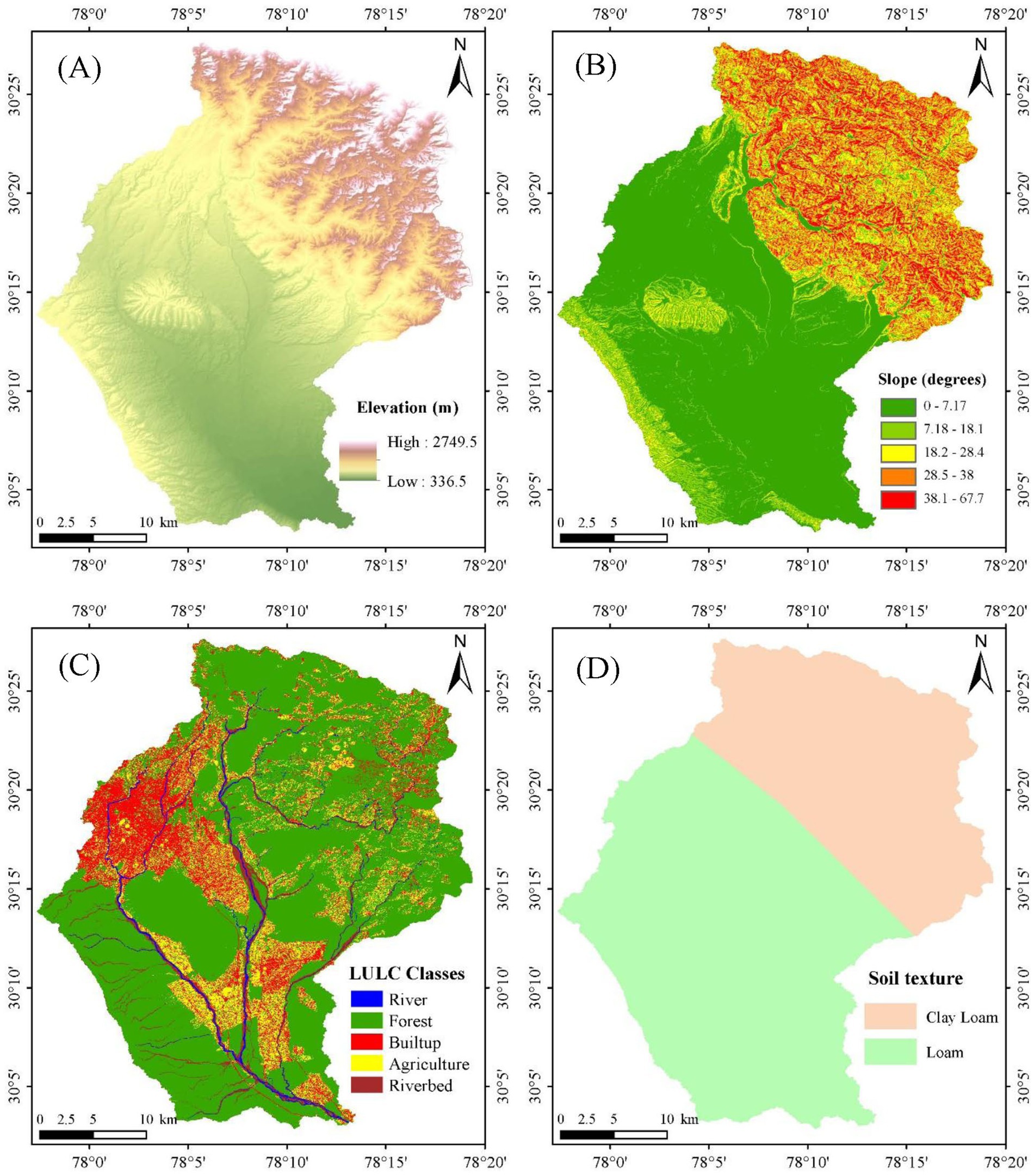
Figure 3. (A) Digital elevation model (DEM) map; (B) Slope map; (C) Land cover map; (D) Soil map used as topographical and spatial input for SWAT model.

The soils property data were obtained from the Harmonized World Soil Database (HWSD) version 1.2, available from the Food and Agriculture Organization (FAO). Based on this data, soils in the basin were classified as clay loam and loam, providing crucial information for modeling soil-water interactions (Figure 3D). Additionally, Figure 2 illustrates the hydrological modeling framework of the study area, demonstrating the interaction of inputs such as precipitation and land use with watershed attributes like soil, topography, and river systems. This flow diagram emphasizes how these elements converge to generate outputs such as streamflow and sediment yield, as simulated by the SWAT model, offering an integrated perspective on the hydrological dynamics of the Song River watershed (Figure 3).

2.2.2 Hydro-meteorological database

In hydrological modeling, precipitation and air temperature are the fundamental meteorological datasets required for model setup. This study utilized gridded precipitation and minimum and maximum air temperature data on a daily scale, obtained from the India Meteorological Department (IMD), with spatial resolutions of 0.25° x 0.25° and 1° x 1°, respectively.

The observed streamflow data required for calibrating the SWAT hydrological model. The Central Water Commission (CWC), India’s central water resource management organization maintained a Gauging and Discharge (G&D) station on the Song River until 2004 at Satyanarayana, located just before the song river’s confluence with the Ganga near Rishikesh. For this study, daily streamflow data spanning 44 years (1971–2004) was obtained from the CWC’s Satyanarayana gauging site, designated as site-2.

Accurately simulating streamflow and sediment dynamics in recent scenario, a weekly monitoring program was conducted at Site 1 and Site 2 over a period of two monsoon years (June 2022 to November 2023). During this period, weekly discharge measurements were carried out using an Acoustic Doppler Current Profiler (ADCP) instrument to ensure high accuracy. Additionally, one-liter water samples were collected during each site visit for laboratory analysis. Water quality analyses were performed at the National Institute of Hydrology, Roorkee water quality laboratory to determine Total Suspended Solids (TSS) concentrations, expressed in mg/L. These analyses provided critical data for calibrating and validating the suspended sediment component of the SWAT model (Table 1).

Table 1

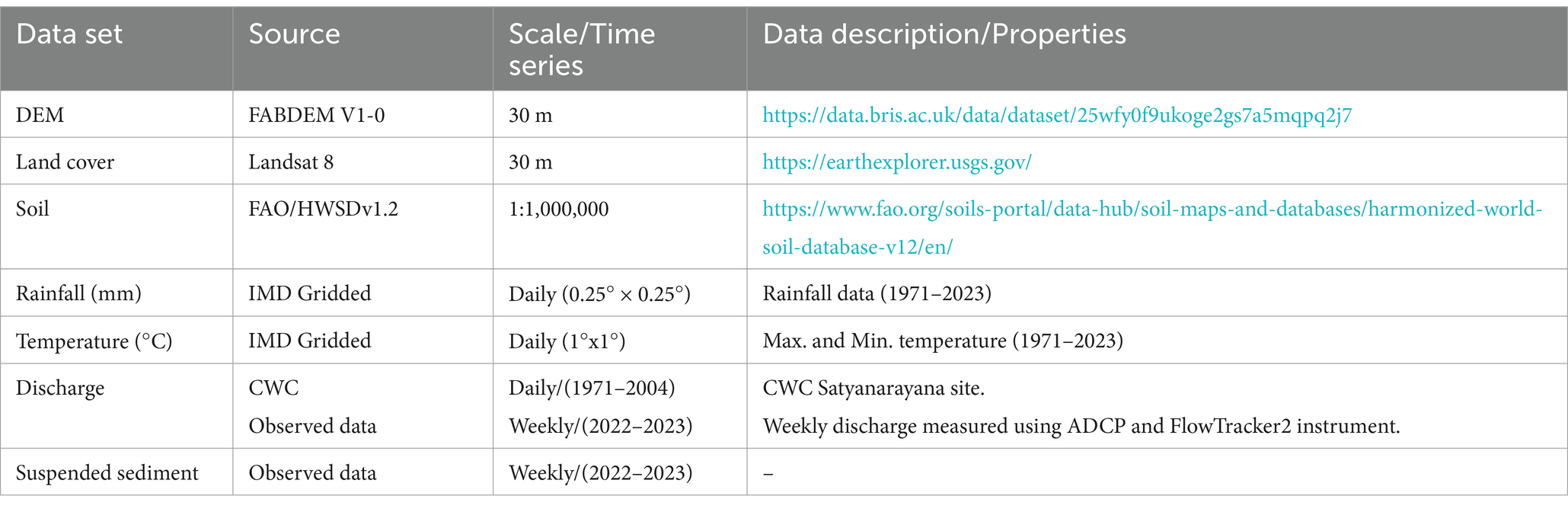
Table 1. Summary of the dataset used in this study.

2.2.3 Field survey and investigation

In the present study, discharge data were available only up to 2004. To address this data gap and validate the model’s applicability for recent conditions, river discharge measurements were conducted for more recent periods, specifically 2022–2023. The process of site selection and the methodology employed for discharge measurement are delineated in sections 3.1.4 and 3.1.5. This approach was essential to ensure that the model’s predictions remain relevant and accurate for contemporary river conditions, considering potential changes in discharge patterns over time.

2.2.4 Design of monitoring programme

The Song River and its primary tributary, the Suswa River, were monitored across two monsoon seasons (June 2022 to November 2023) at two strategically selected sites along the Song River. These stations were situated upstream and downstream of the confluence of the Suswa River, adjacent to road bridges, ensuring accessibility during the monsoon season. Discharge measurements were conducted weekly during the monsoon (June to September), biweekly during the post-monsoon period (October to November), and monthly during the lean seasons (December to May). Table 2 provides details of the monitoring stations.

Table 2

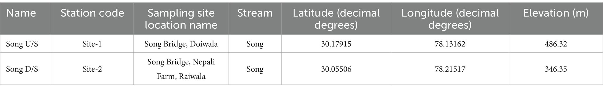
Table 2. Descriptive characteristics of the selected monitoring stations.

2.2.5 Observed streamflow and sediment data

Flow velocity and discharge measurements were conducted using two instruments: the SonTek FlowTracker2 and the Acoustic Doppler current profiler (ADCP). The SonTek FlowTracker2, an Acoustic Doppler Velocimeter (ADV), utilizes the Doppler effect to measure velocities ranging from 0.001 to 4 m/s. For low-flow conditions, the ADV was employed to measure velocity, while the mid-section method was utilized to calculate river discharge. In flood scenarios, a boat-mounted ADCP was deployed to measure both velocity and discharge (Figure 4).

Figure 4

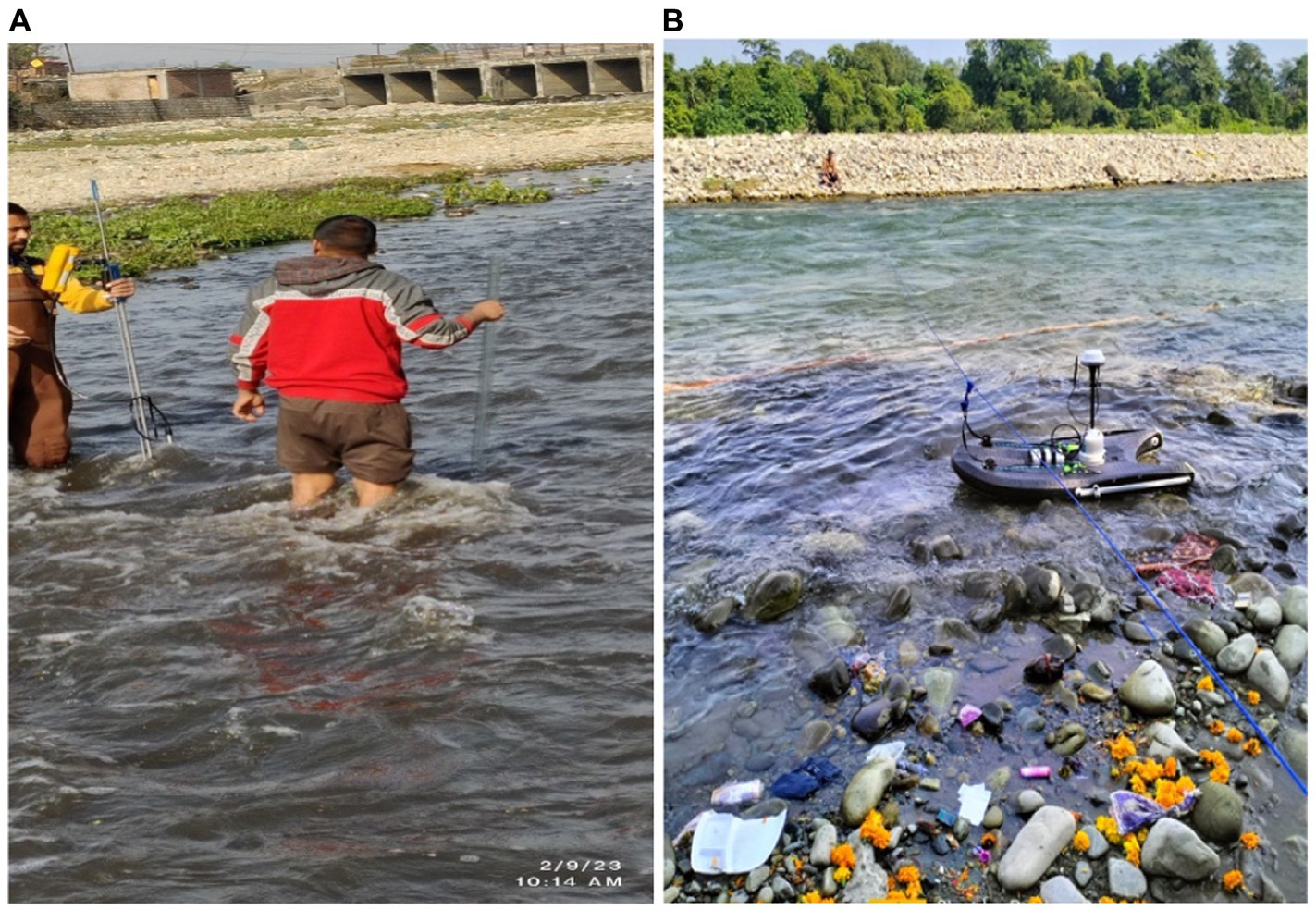
Figure 4. Discharge measurement using (A) Flow-Tracker2 in low flow condition (B) ADCP in high flow condition.

Water samples for sediment analysis were collected during each site visit. At all monitoring locations, river water samples were collected using the grab sampling technique. One liter of river water sample was collected in high-density polyethylene (HDPE) containers and transport to the National Institute of Hydrology, Roorkee water quality lab for examination. To ensure uniformity, the collected samples were vigorously agitated. Subsequently, one liter of each sample was filtered through a 0.45-micron gridded cellulose nitrate membrane using an electric vacuum pump to extract suspended sediments. The filter paper containing the captured sediments was then dried in a hot oven to determine the total suspended sediment (TSS) concentration. The TSS concentration in the water sample was calculated by measuring the dry weight difference of the filter paper before and after the filtration process.

2.3 Model setup

The eco-hydrological model Soil and Water Assessment Tool (SWAT) is a versatile hydrological model capable of simulating diverse environmental conditions and scales (Arnold et al., 1998). The establishment of a SWAT model requires spatially distributed data, including Digital Elevation Models (DEMs), soil data, land use land cover maps, and weather data. The model operates exclusively on this data and does not necessitate prior knowledge of catchment behavior or flow processes. SWAT simulates water balance, a fundamental driver of watershed processes, to accurately predict runoff, sediment, and nutrient movement. The model comprises two primary components: the land phase and the routing phase. For surface runoff estimation, the Curve Number method is utilized.

2.4 Model calibration and validation and sensitivity analysis

The SWAT model encompasses numerous hydrological parameters whose effectiveness is affected by variables such as soil type, slope, and land cover. To identify the most influential parameters and reduce the number needed for calibration, sensitivity analysis is essential. This research employed the SUFI-2 algorithm within the SWAT-CUP interface to perform sensitivity analysis on 13 crucial parameters, including ALPHA_BF (baseflow alpha factor), CH_K2 (hydraulic conductivity in the main channel alluvium), CH_N2 (Manning’s “n” for the main channel), as well as GWQMN, SOL_AWC, ESCO, and SURLAG. The impact of these parameters on hydrological components like discharge, infiltration, baseflow, groundwater flow, evaporation, and transpiration were examined by methodically altering one parameter at a time while keeping others constant. The relationship between parameters and hydrological responses was quantified using sensitivity coefficients. To enhance the model’s accuracy, both manual and automated calibration techniques were utilized. Manual calibration involved visually adjusting parameters based on observed and simulated flow patterns, considering catchment characteristics. Automated calibration, facilitated by SWAT-CUP, systematically optimized uncertain parameters by comparing model outputs with measured data through an interactive interface. This combined approach ensured effective parameter optimization and improved the SWAT model’s ability to simulate hydrological processes.

2.5 Performance evaluation

There are multiple efficacy measures that can be used to assess the model’s performance. These efficacy metrics show how the model-simulated values and the observed values are reconciled. Nash-Sutcliffe Efficiency (NSE) (Equation 1), coefficient of determination (R²) (Equation 2) and PBIAS (Equation 3) are the most widely utilized metrics among them (Sane et al., 2020; Swain et al., 2022).

Nash-Sutcliffe efficiency (NSE) (Nash and Sutcliffe, 1970),

$\begin{array}{ll}\mathrm{N}\mathrm{S}\mathrm{E}=1-\frac{{{\displaystyle \sum }}_{i=1}^n{\left(O_i-P_i\right)}^2}{{{\displaystyle \sum }}_{\mathrm{i}=1}^n{\left(O_i-\overline{O}\right)}^2}& (1)\end{array}$

Percent bias (PBIAS) (Moriasi et al., 2007),

$\begin{array}{ll}\mathit{PBIAS}=\frac{\left({{\displaystyle \sum }}_{i=1}^n\left(O_i-P_i\right)\times 100\right)}{\left({{\displaystyle \sum }}_{i=1}^n{O}_i\right)}& (2)\end{array}$

Coefficient of determination (R²) (Suryavanshi et al., 2017),

$\begin{array}{ll}{R}^2={\left[\frac{{{\displaystyle \sum }}_{i=1}^n\left(O_i+\overline{O}\right)\left(P_i-\overline{P}\right)}{{{\displaystyle \sum }}_{i=1}^n{\left(O_i-\overline{O}\right)}^2{{\displaystyle \sum }}_{i=1}^n{\left(P_i-\overline{P}\right)}^2}\right]}^2& (3)\end{array}$

P_i and O_i are the simulated and observed values of discharge; n is the sample number,

$\overline{P}$ and $\overline{O}$ are the average of simulated and observed discharge.

3 Results and discussion

3.1 Model calibration and validation and sensitivity analysis

This research utilized previous studies to guide parameter selection for calibration, examining 13 parameters in total, with 8 identified as sensitive at a 0.05 significance level. Table 3 outlines the range, fitted values, t-statistics, significance levels, and sensitivity rankings for these parameters. The study employed a three-year warm-up period (1971–1973), with calibration and validation periods spanning 1974–1995 and 1996–2004, respectively. The dotty plots generated in SWAT-CUP indicate that the baseflow recession constant (ALPHA_BF) and Channel roughness (CH_N2) are the most sensitive parameters. This conclusion is evident from the noticeable variation in the model’s performance metrics corresponding to changes in their values. The ALPHA_BF was calibrated to 0.05, suggesting a contribution of groundwater to streamflow, during low-flow periods is a critical factor in accurately simulating streamflow. CH_N2 was set at 0.04, indicative of a dredged channel, while effective hydraulic conductivity (CH_K2) was calibrated to 121.15 mm/h, signifying high-permeability conditions. The return flow threshold depth (GWQMN) was set at 735 mm, and soil water capacity (SOL_AWC) showed a 47% decrease, indicating reduced plant-available water. The groundwater “revap” coefficient (GW_REVAP) was calibrated to 0.07, suggesting limited water movement to the root zone. Manning’s coefficient (OV_N) was determined to be 0.83, and deep aquifer percolation (REVAPM) required 404.5 mm of shallow aquifer water. Soil evaporation compensation (ESCO) was set at 0.12, indicating high demand from lower soil layers. Surface runoff lag time (SURLAG) was calibrated to 2.33, and plant uptake compensation (EPCO) decreased to −0.29, demonstrating reduced uptake in lower soil layers. Groundwater delay (GW-DELAY) was established at 472.5 days, indicating a slow aquifer response, while lateral flow travel time (LAT_TTIME) was set at 22.14 days, representing lateral flow dynamics within the hydrological response units (HRUs). These calibrated parameters significantly enhanced model performance and improved the simulation of hydrological processes.

Table 3

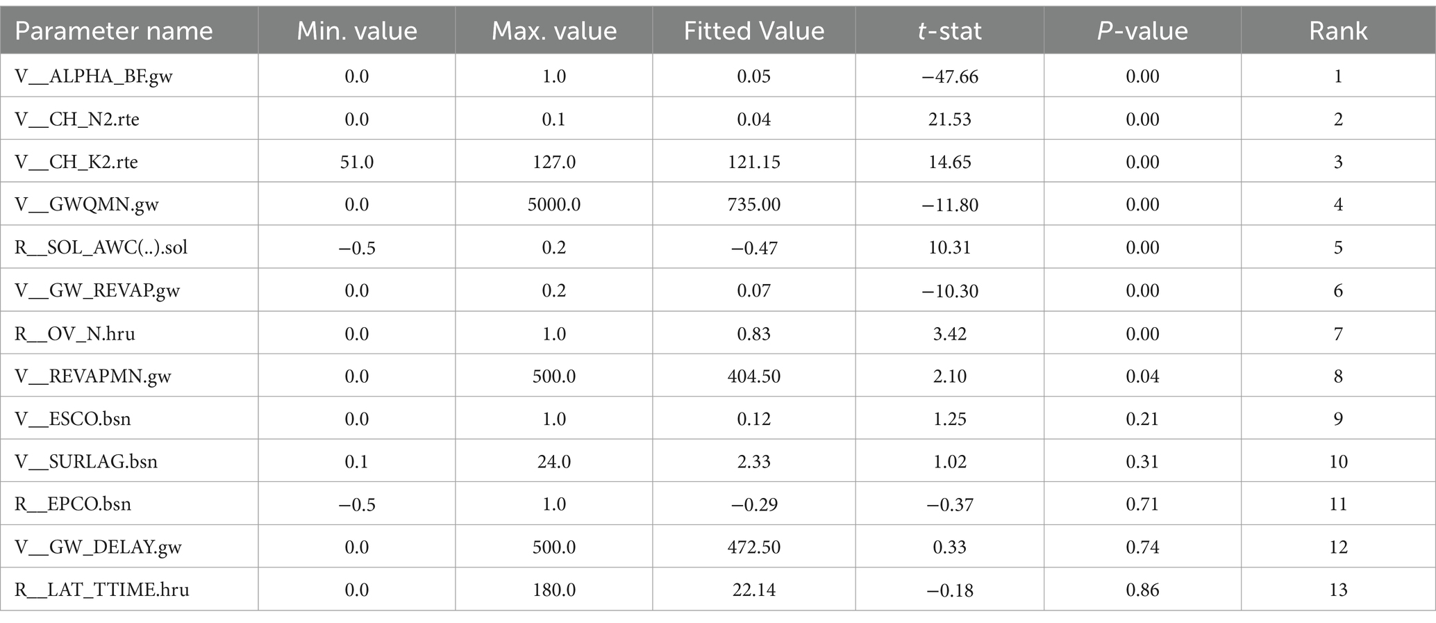
Table 3. Fitted values of the SWAT parameter and statistics of sensitivity analysis.

3.2 Model performance evaluation

The study employed daily observations from 1974 to 2004, with Figure 5 illustrating the temporal comparison between observed and simulated discharge during both calibration and validation phases. Model effectiveness was assessed using R², NSE, and PBIAS metrics, as presented in Table 4. The observed and simulated flows showed strong correlation, with R² values of 0.79 and 0.66 for calibration and validation, respectively. During calibration, both baseflow and peak flows aligned well between observed and simulated data. Although the validation period showed underestimated goodness of fit, the results remained satisfactory. The NSE reached 0.7 during calibration and 0.62 during validation. PBIAS values fell within acceptable ranges for both periods, measuring 17.06 for calibration and 19.60 for validation.

Figure 5

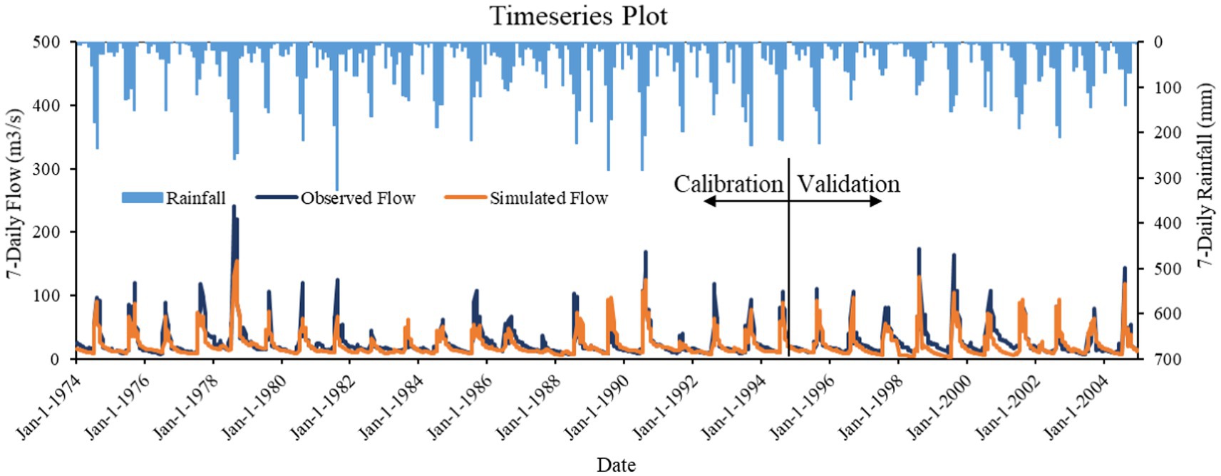
Figure 5. Time series plot of weekly mean observed and simulated flow (1974–2004) at site 2 maintained by CWC.

Table 4

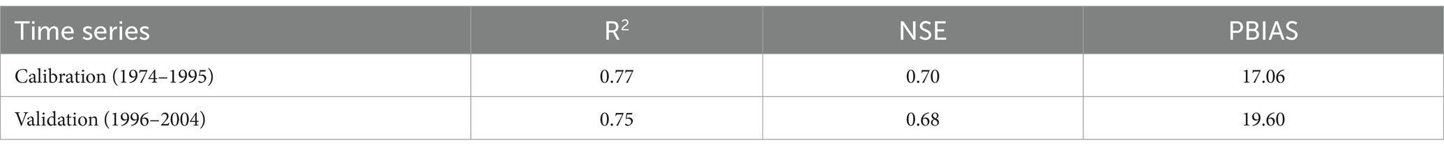
Table 4. Model performance statistics.

The weekly average simulated and observed flow for the 1974–2004 period is depicted in Figure 5 as a time series plot. This graph reveals a high degree of similarity between the simulated and observed discharge, with the model successfully capturing overall flow trends, including seasonal fluctuations and high-flow events. The simulated flow closely tracks the observed data during the calibration phase, demonstrating the model’s precision in replicating both low-flow conditions and peak discharge occurrences. Although the validation period exhibits minor underestimations of some peak flows, the general trend remains aligned, indicating satisfactory model performance across the extended timeframe. This sustained consistency underscores the model’s dependability for long-term hydrological flow simulations.

Figure 6 presents a scatter plot depicting the weekly mean simulated versus observed flow during the calibration and validation periods. The plot demonstrates a strong linear relationship between the simulated and observed flow data, with the majority of points clustering in close proximity to the 1:1 line, indicating a high degree of accuracy in the model’s predictions. During the calibration period, the scatter plot exhibits a tight correlation, reflecting the model’s efficacy in capturing the observed flow dynamics. Although the validation period displays a slight dispersion from the 1:1 line, the overall alignment remains satisfactory, confirming the model’s robustness in simulating streamflow across diverse hydrological conditions.

Figure 6

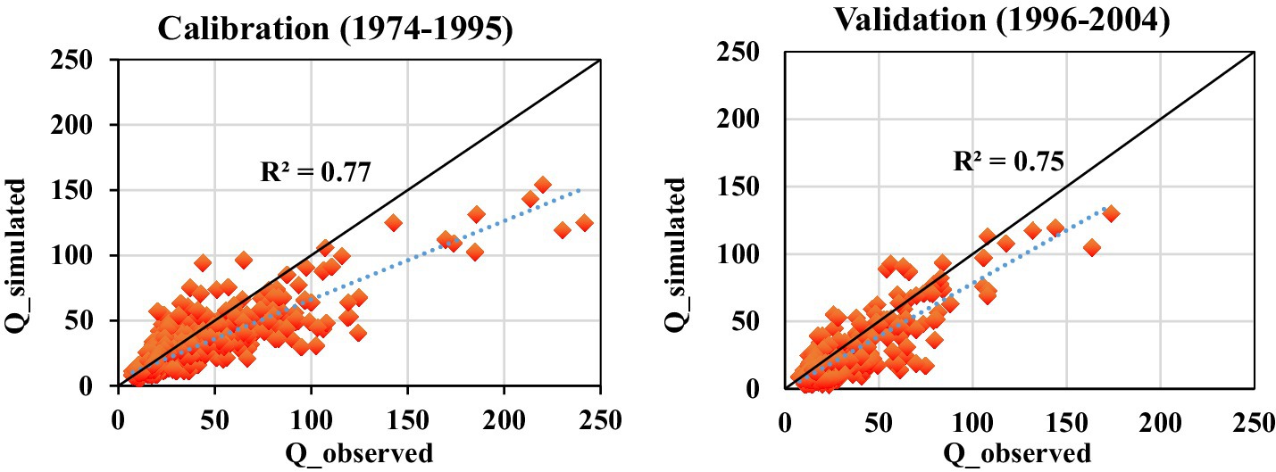
Figure 6. Scatter plot of weekly mean simulated and observed flow during calibration and validation.

3.3 Model performance evaluation with field survey data

The model’s applicability to the study area was evaluated by comparing its simulated flows with ADCP-measured discharges obtained during a field survey. A strong correlation was observed between the simulated flows and observed discharge data at both upstream (site-1) and downstream (site-2) locations. The model’s performance was quantified using statistical indicators R², NSE, and PBIAS, with results presented in Table 5, demonstrating its robust performance. The R² values, ranging from 0.78 to 0.79, indicated a strong correlation, while NSE values of 0.79 upstream and 0.68 downstream showed high agreement between simulated and observed flows. PBIAS values of 0.04 upstream and − 16.20 downstream fell within acceptable ranges, further confirming the model’s reliability. A time series plot comparing weekly mean simulated flows with observed flows for 2022–2023 at both sites is shown in Figure 7. The plot reveals exceptional alignment at the upstream site, where the model accurately captures flow variations and peak flows. Although minor discrepancies are noted at the downstream site, the overall flow patterns are well-represented, highlighting the model’s ability to accurately simulate flow conditions in the Song River basin under diverse field conditions.

Table 5

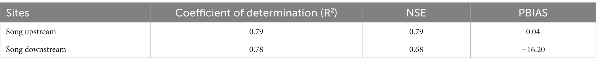
Table 5. Performance of calibrated model with field survey data.

Figure 7

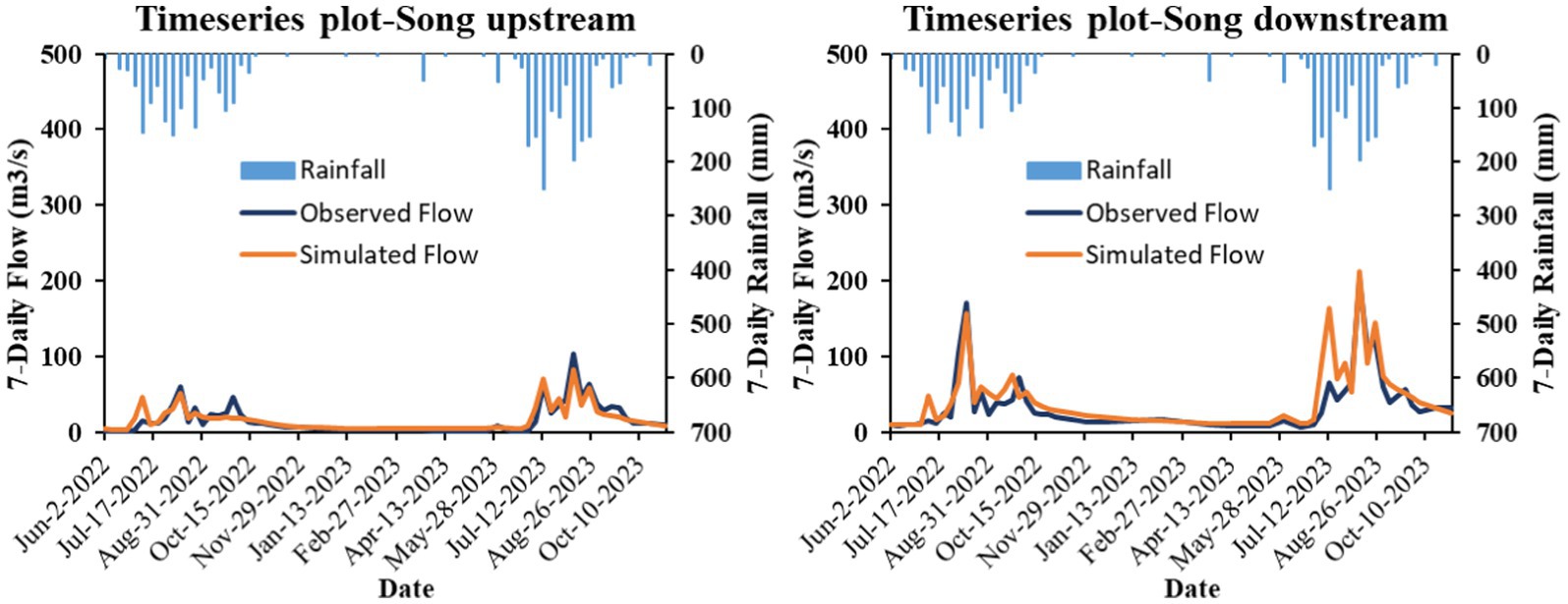
Figure 7. Time series plot of the weekly mean simulated flow and field survey observed flow (2022–2023) at the upstream and downstream sections of the Song River.

Figure 8 presents a scatter plot depicting the relationship between weekly mean simulated flow and field survey observed flow at both the upstream and downstream sections of the Song River. The plot demonstrates a strong correlation between the simulated and observed data, with data points closely aligned with the line of perfect agreement. The upstream section exhibits a marginally higher degree of concordance, indicating superior model accuracy in this region, while the downstream section, despite displaying some dispersion, still demonstrates robust predictive performance. In aggregate, the scatter plot corroborates the model’s efficacy in replicating observed flow conditions across distinct sections of the river.

Figure 8

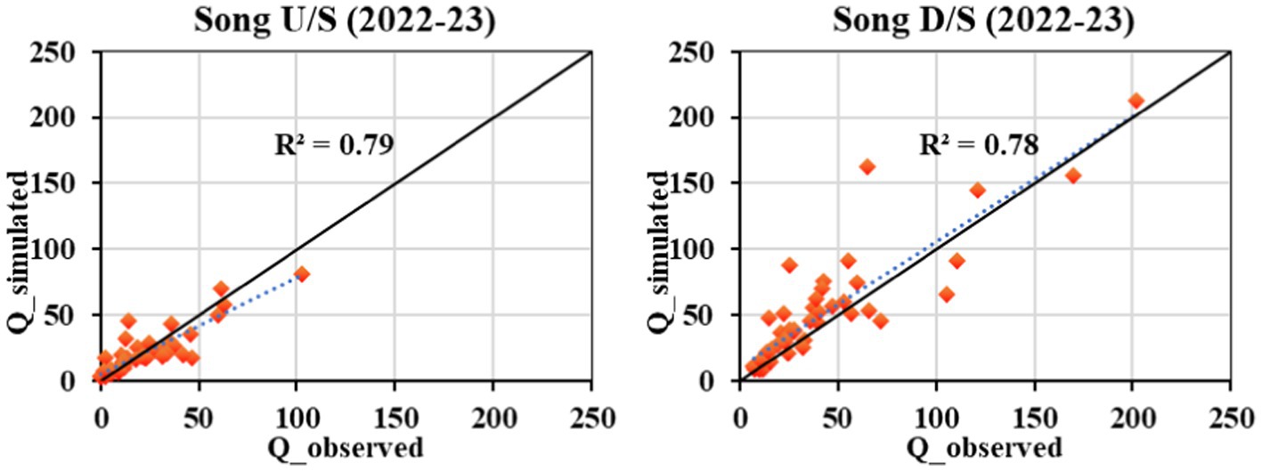
Figure 8. Scatter plot of weekly mean simulated flow and field survey observed flow at upstream and downstream of Song River.

3.4 Model calibration and validation for weekly sediment load

The pre-calibrated runoff model was subsequently utilized for sediment load calibration. Four additional parameters Channel erodibility factor (CH_EROD), Peak rate adjustment factor for sediment routing in the subbasin (ADJ_PKR), USLE equation support practice (P) factor (USLE_P) and Linear parameter for calculating the maximum amount of sediment (SPCON) added in SWAT-CUP using SUFI2 algorithm for calibrate and validate Sediment load, at daily time scale (Table 6). The results of the best simulation (based on efficacy measures on daily scale) and its comparison with respect to the observed sediment load along with the observed discharge at weekly scale for 2 years, i.e., 2023–2024 are presented in Figure 9. The statistical performance indicators for the calibration period (2022) revealed that the model achieved an R² value of 0.70 and a Nash-Sutcliffe Efficiency (NSE) of 0.53. For the validation period (2023), the model demonstrated an R² of 0.59 and an NSE of 0.52.

Figure 9

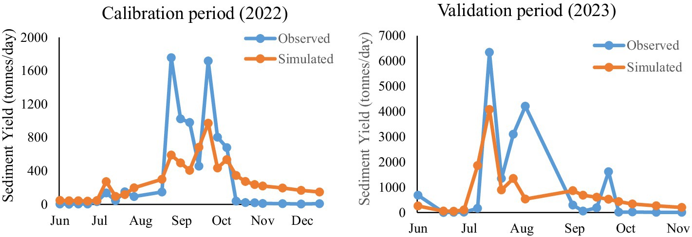
Figure 9. Sediment load calibration and validation plot at Song D/S.

Table 6

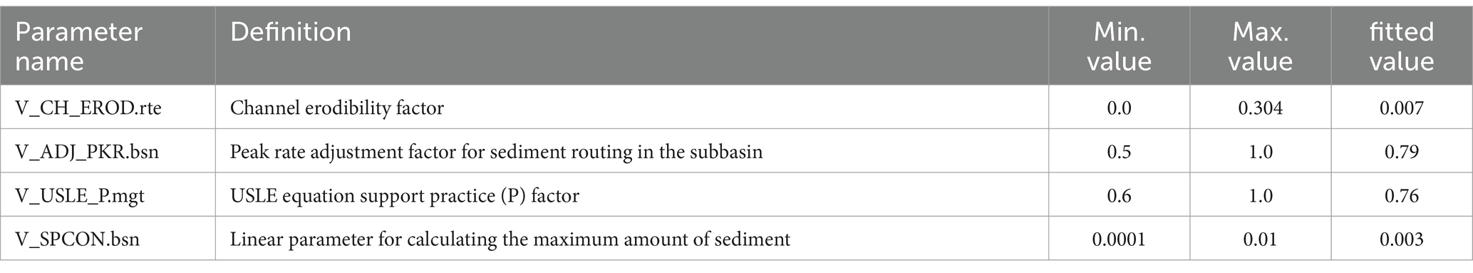
Table 6. Fitted values of the SWAT parameter for sediment analysis.

Figure 9, comparing observed and simulated daily sediment yields at site 2 during the 2022 calibration and 2023 validation periods, elucidates both the efficacy and limitations of the SWAT model. In the 2022 calibration period, observed sediment yields exhibit substantial peaks in September and October, with loads reaching up to 1,800 tonnes per day. While the SWAT model captures the overall seasonal pattern, including the pronounced increase during the monsoon and subsequent decline, it underestimates the magnitude of these peaks, particularly during high-flow events. Similarly, during the 2023 validation period, the observed sediment yield peaks in July, exceeding 6,000 tonnes per day, followed by a rapid decline and smaller peaks in subsequent months. The simulated sediment yield generally follows this trend but significantly underestimates the July peak, reaching only approximately 4,000 tonnes per day, and fails to capture some of the acute fluctuations observed in the following months. These results demonstrate the model’s capacity to replicate the general seasonal dynamics of sediment transport but also underscore challenges in accurately simulating extreme events. To enhance the model’s performance, particularly during high-flow periods, further refinement of parameters or the incorporation of additional factors may be necessary.

4 Conclusion

The present study demonstrates the efficacy of the SWAT model in simulating streamflow and sediment yield within the Song River watershed, establishing its reliability for hydrological modelling in comparable basins. A comprehensive runoff calibration and validation process refined 13 critical parameters, with 8 identified as highly sensitive, significantly enhancing the model’s accuracy. During the calibration phase (1974–1995), the model achieved an R² of 0.79 and a NSE of 0.70, indicating a robust correlation between simulated and observed discharge capture both baseflow and peak flow dynamics with high precision. Although a slight decrease in performance occurred during the validation period (1996–2004), with R² and NSE values of 0.66 and 0.62, demonstrating its robustness across varying conditions suggesting the model maintains efficacy under changing conditions, such as alterations in land use and climate. The Percent Bias (PBIAS) values of 17.06% during calibration and 19.60% during validation indicated underestimate the model. Furthermore, real-time observed field data from 2022–2023 reinforced the model’s accuracy, with strong correlations (R² = 0.79 upstream and 0.78 downstream), validating its applicability for watershed management and planning.

In addition to streamflow, the model was evaluated for sediment transport, successfully capturing seasonal trends in sediment dynamics. The R² and NSE value for weekly sediment yield at site 2 was obtained as 0.70 and 0.53, respectively, for the calibration period and 0.59 and 0.52, respectively, for the validation period. However, the model underestimated sediment yields at site 2 during high-flow events, indicating the necessity for further refinement to enhance predictions under extreme weather conditions, such as floods. Notwithstanding this limitation, the model’s capability to simulate sediment transport remains valuable for comprehending sediment dynamics and addressing sediment-related issues in watershed management.

The calibration and validation results indicate that the model performs well in simulating streamflow and provides satisfactory results for sediment transport. However, the limited availability of observed suspended sediment data remains a significant challenge for achieving a more reliable and persuasive model application. The calibrated model has also been utilized to simulate nonpoint source pollution loads in the Song River catchment. With ongoing refinement and the incorporation of additional field data, the model exhibits substantial potential to improve hydrological modelling and support more effective water resource management strategies in the future.

Data availability statement

The raw data supporting the conclusions of this article will be made available by the authors, without undue reservation.

Author contributions

SQ: Writing – original draft, Writing – review & editing. PK: Writing – review & editing. HS: Writing – original draft.

Funding

The author(s) declare financial support was received for the research, authorship, and/or publication of this article. This study was supported by the National Institute of Hydrology Roorkee, Uttarakhand, India.

Acknowledgments

The authors are thankful to the National Institute of Hydrology Roorkee, Uttarakhand as well as Central University of Jharkhand, Ranchi-India for providing necessary laboratory work to conduct the research work.

Conflict of interest

The authors declare that the research was conducted in the absence of any commercial or financial relationships that could be construed as a potential conflict of interest.

Publisher’s note

All claims expressed in this article are solely those of the authors and do not necessarily represent those of their affiliated organizations, or those of the publisher, the editors and the reviewers. Any product that may be evaluated in this article, or claim that may be made by its manufacturer, is not guaranteed or endorsed by the publisher.

Supplementary material

The Supplementary material for this article can be found online at: https://www.frontiersin.org/articles/10.3389/frwa.2025.1500086/full#supplementary-material

References

Aawar, T., and Khare, D. (2020). Assessment of climate change impacts on streamflow through hydrological model using SWAT model: a case study of Afghanistan. Modeling Earth Syst. Environ. 6, 1427–1437. doi: 10.1007/s40808-020-00759-0

Crossref Full Text | Google Scholar

Agrawal, N., Verma, M. K., and Tripathi, M. P. (2011). Hydrological modelling of chhokranala watershed using weather generator with SWATmodel. Ind. J. Soil Conserv. 39, 89–94.

Google Scholar

Arnold, J. G., and Allen, P. M. (1996). Estimating hydrologic budgets for three Illinois watersheds. J. Hydrol. 176, 57–77. doi: 10.1016/0022-1694(95)02782-3

Crossref Full Text | Google Scholar

Arnold, J. G., Srinivasan, R., Muttiah, R. S., and Williams, J. R. (1998). Large area hydrologic modeling and assessment part I: model development 1. JAWRA 34, 73–89. doi: 10.1111/j.1752-1688.1998.tb05961.x

Crossref Full Text | Google Scholar

Bouslihim, Y., Kacimi, I., Brirhet, H., Khatati, M., Rochdi, A., Pazza, N. E. A., et al. (2016). Hydrologic modeling using SWAT and GIS, application to subwatershed Bab-Merzouka (Sebou, Morocco). J. Geogr. Inf. Syst. 8, 20–27. doi: 10.4236/jgis.2016.81002

Crossref Full Text | Google Scholar

Brutsaert, W., and Parlange, M. B. (1998). Hydrologic cycle explains the evaporation paradox. Nature 396:30. doi: 10.1038/23845

Crossref Full Text | Google Scholar

Daggupati, P., Pai, N., Ale, S., Douglas-Mankin, K. R., Zeckoski, R. W., Jeong, J., et al. (2015). A recommended calibration and validation strategy for hydrologic and water quality models. Trans. ASABE 58, 1705–1719. doi: 10.13031/trans.58.10712

PubMed Abstract | Crossref Full Text | Google Scholar

Folton, N., Andréassian, V., and Duperray, R. (2015). Hydrological impact of forest-fire from paired-catchment and rainfall–runoff modelling perspectives. Hydrol. Sci. J. 60, 1213–1224. doi: 10.1080/02626667.2015.1035274

Crossref Full Text | Google Scholar

Gassman, P. W., Sadeghi, A. M., and Srinivasan, R. (2014). Applications of the SWAT model special section: overview and insights. J. Environ. Qual. 43, 1–8. doi: 10.2134/jeq2013.11.0466

PubMed Abstract | Crossref Full Text | Google Scholar

Gelete, G., Nourani, V., Gokcekus, H., and Gichamo, T. (2023). Ensemble physically based semi-distributed models for the rainfall-runoff process modeling in the data-scarce Katar catchment, Ethiopia. J. Hydroinform. 25, 567–592. doi: 10.2166/hydro.2023.197

Crossref Full Text | Google Scholar

Ghoraba, S. M. (2015). Hydrological modeling of the Simly dam watershed (Pakistan) using GIS and SWAT model. Alex. Eng. J. 54, 583–594. doi: 10.1016/j.aej.2015.05.018

Crossref Full Text | Google Scholar

Gupta, A., Hantush, M. M., Govindaraju, R. S., and Beven, K. (2024). Evaluation of hydrological models at gauged and ungauged basins using machine learning-based limits-of-acceptability and hydrological signatures. J. Hydrol. 641:131774. doi: 10.1016/j.jhydrol.2024.131774

Crossref Full Text | Google Scholar

Hassan, M. A., Church, M., Yan, Y., and Slaymaker, O. (2010). Spatial and temporal variation of in-reach suspended sediment dynamics along the mainstem of Changjiang (Yangtze River), China. Water Res. Res. 46:9228. doi: 10.1029/2010WR009228

PubMed Abstract | Crossref Full Text | Google Scholar

Iwanaga, T., Partington, D., Ticehurst, J., Croke, B. F., and Jakeman, A. J. (2020). A socio-environmental model for exploring sustainable water management futures: participatory and collaborative modelling in the lower Campaspe catchment. J. Hydrol. Reg. Stu. 28:100669. doi: 10.1016/j.ejrh.2020.100669

Crossref Full Text | Google Scholar

Jain, S. K., Tyagi, J., and Singh, V. (2010). Simulation of runoff and sediment yield for a Himalayan watershed using SWAT model. J. Water Res. Prot. 2, 267–281. doi: 10.4236/jwarp.2010.23031

Crossref Full Text | Google Scholar

Janjić, J., and Tadić, L. (2023). Fields of application of SWAT hydrological model—a review. Earth 4, 331–344. doi: 10.3390/earth4020018

Crossref Full Text | Google Scholar

Joseph, J., Ghosh, S., Pathak, A., and Sahai, A. K. (2018). Hydrologic impacts of climate change: comparisons between hydrological parameter uncertainty and climate model uncertainty. J. Hydrol. 566, 1–22. doi: 10.1016/j.jhydrol.2018.08.080

Crossref Full Text | Google Scholar

Kaur, T., and Sinha, A. K. (2019). Pesticides in agricultural run offs affecting water resources: a study of Punjab (India). Agric. Sci. 10, 1381–1395. doi: 10.4236/as.2019.1010101

Crossref Full Text | Google Scholar

Koltsida, E., Mamassis, N., and Kallioras, A. (2023). Hydrological modeling using the soil and water assessment tool in urban and peri-urban environments: the case of Kifisos experimental subbasin (Athens, Greece). Hydrol. Earth Syst. Sci. 27, 917–931. doi: 10.5194/hess-27-917-2023

Crossref Full Text | Google Scholar

Kumar, V., and Paramanik, S. (2020). Application of high-frequency spring discharge data: a case study of Mathamali spring rejuvenation in the Garhwal Himalaya. Water Supply 20, 3380–3392. doi: 10.2166/ws.2020.223

Crossref Full Text | Google Scholar

Kumar, V., and Sen, S. (2023). Hydrometeorological field instrumentation in lesser Himalaya to advance research for future water and food security. Environ. Monit. Assess. 195:1162. doi: 10.1007/s10661-023-11625-8

PubMed Abstract | Crossref Full Text | Google Scholar

Kumar, V., and Sen, S. (2024). Rating curve development and uncertainty analysis in mountainous watersheds for informed hydrology and resource management. Front. Water 5:1323139. doi: 10.3389/frwa.2023.1323139

Crossref Full Text | Google Scholar

Mishra, R. R., and Saxena, S. (2024). “Cities and rivers: a symbiotic relationship” in Managing Urban Rivers (Amsterdam: Elsevier), 3–24.

Google Scholar

Moriasi, D. N., Arnold, J. G., Van Liew, M. W., Bingner, R. L., Harmel, R. D., and Veith, T. L. (2007). Model evaluation guidelines for systematic quantification of accuracy in watershed simulations. Trans. ASABE 50, 885–900. doi: 10.13031/2013.23153

Crossref Full Text | Google Scholar

Narsimlu, B., Gosain, A. K., Chahar, B. R., Singh, S. K., and Srivastava, P. K. (2015). SWAT model calibration and uncertainty analysis for streamflow prediction in the Kunwari River basin, India, using sequential uncertainty fitting. Environ. Process. 2, 79–95. doi: 10.1007/s40710-015-0064-8

Crossref Full Text | Google Scholar

Nash, J. E., and Sutcliffe, J. V. (1970). River flow forecasting through conceptual models’ part I—A discussion of principles. J. Hydrol. 10, 282–290. doi: 10.1016/0022-1694(70)90255-6

Crossref Full Text | Google Scholar

Nguyen, H. Q., and Kappas, M. (2015). Modeling surface runoff and evapotranspiration using SWAT and beach for a tropical watershed in North Vietnam, compared to MODIS products. Int. J. Adv. Remote Sens. GIS 4, 1367–1384. doi: 10.23953/cloud.ijarsg.124

Crossref Full Text | Google Scholar

Pérez-Sánchez, J., Senent-Aparicio, J., Segura-Méndez, F., Pulido-Velazquez, D., and Srinivasan, R. (2019). Evaluating hydrological models for deriving water resources in peninsular Spain. Sustain. For. 11:2872. doi: 10.3390/su11102872

Crossref Full Text | Google Scholar

Phuong, T. T., Thong, C. V. T., Ngoc, N. B., and Van Chuong, H. (2014). Modeling soil erosion within small mountainous watershed in Central Vietnam using GIS and SWAT. Resour. Environ 4, 139–147. doi: 10.5923/j.re.20140403.02

Crossref Full Text | Google Scholar

Rafiei Emam, A., Kappas, M., Linh, N. H. K., and Renchin, T. (2017). Hydrological modeling and runoff mitigation in an ungauged basin of Central Vietnam using SWAT model. Hydrology 4:16. doi: 10.3390/hydrology4010016

Crossref Full Text | Google Scholar

Sahu, M., Lahari, S., Gosain, A. K., and Ohri, A. (2016). Hydrological modeling of Mahi basin using SWAT. J. Water Res. Hydraulic Eng. 5, 68–79. doi: 10.5963/JWRHE0503001

Crossref Full Text | Google Scholar

Samimi, M. (2020). Adaptive agricultural water resources Management in a Desert River Basin: Insights from hydrologic modeling. Stillwater, OK: Oklahoma State University.

Google Scholar

Sane, M. L., Sambou, S., Leye, I., Ndione, D. M., Diatta, S., Ndiaye, I., et al. (2020). Calibration and validation of the SWAT model on the watershed of Bafing River, Main upstream tributary of Senegal River: checking for the influence of the period of study. Open J. Modern Hydrol. 10, 81–104. doi: 10.4236/ojmh.2020.104006

Crossref Full Text | Google Scholar

Schuol, J., Abbaspour, K. C., Yang, H., Srinivasan, R., and Zehnder, A. J. (2008). Modelling blue and green water availability in Africa. Water Resour. Res. 44:6609. doi: 10.1029/2007WR006609

Crossref Full Text | Google Scholar

Seneviratne, S. I., Corti, T., Davin, E. L., Hirschi, M., Jaeger, E. B., Lehner, I., et al. (2010). Investigating soil moisture–climate interactions in a changing climate: a review. Earth Sci. Rev. 99, 125–161. doi: 10.1016/j.earscirev.2010.02.004

Crossref Full Text | Google Scholar

Suryavanshi, S., Pandey, A., and Chaube, U. C. (2017). Hydrological simulation of the Betwa River basin (India) using the SWAT model. Hydrol. Sci. J. 62, 960–978. doi: 10.1080/02626667.2016.1271420

Crossref Full Text | Google Scholar

Swain, S., Mishra, S. K., Pandey, A., Pandey, A. C., Jain, A., Chauhan, S. K., et al. (2022). Hydrological modelling through SWAT over a Himalayan catchment using high-resolution geospatial inputs. Environ. Challenges 8:100579. doi: 10.1016/j.envc.2022.100579

Crossref Full Text | Google Scholar

Vandenberghe, V., Van Griensven, A., Bauwens, W., and Vanrolleghem, P. A. (2006). Effect of different river water quality model concepts used for river basin management decisions. Water Sci. Technol. 53, 277–284. doi: 10.2166/wst.2006.322

PubMed Abstract | Crossref Full Text | Google Scholar