Convolutional long short-term memory neural network for groundwater change prediction

Patra, Sumriti Ranjan; Chu, Hone-Jay

doi:10.3389/frwa.2024.1471258

ORIGINAL RESEARCH article

Front. Water, 13 November 2024

Sec. Water and Artificial Intelligence

Volume 6 - 2024 | https://doi.org/10.3389/frwa.2024.1471258

Convolutional long short-term memory neural network for groundwater change prediction

$\r\nSumriti Ranjan Patra$ Sumriti Ranjan Patra

Hone-Jay Chu^*

Department of Geomatics, National Cheng Kung University, Tainan City, Taiwan

Forecasting groundwater changes is a crucial step towards effective water resource planning and sustainable management. Conventional models still demonstrated insufficient performance when aquifers have high spatio-temporal heterogeneity or inadequate availability of data in simulating groundwater behavior. In this regard, a spatio-temporal groundwater deep learning model is proposed to be applied for monthly groundwater prediction over the entire Choushui River Alluvial Fan in Central Taiwan. The combination of the Convolution Neural Network (CNN) and Long Short-Term Memory (LSTM) known as Convolutional Long Short-Term Memory (CLSTM) Neural Network is proposed and investigated. Result showed that the monthly groundwater simulations from the proposed neural model were better reflective of the original observation data while producing significant improvements in comparison to only the CNN, LSTM as well as classical neural models. The study also explored the performance of the Masked CLSTM model which is designed to handle missing data by reconstructing incomplete spatio-temporal input images, enhancing groundwater forecasting through image inpainting. The findings indicated that the neural architecture can efficiently extract the relevant spatial features from the past incomplete information of hydraulic head observations under various masking scenarios while simultaneously handling the varying temporal dependencies over the entire study region. The proposed model showed strong reliability in reconstructing and simulating the spatial distribution of hydraulic heads for the following month, as evidenced by low RMSE values and high correlation coefficients when compared to observed data.

1 Introduction

Groundwater is a vital resource of freshwater that is being utilized for a variety of purposes such as agriculture, drinking, and industrial production (Famiglietti, 2014; Kulkarni et al., 2015; Megdal et al., 2015; Mukherjee, 2018). Recently, significant global warming, e.g., rise in global temperature (Sen, 2009; Zhang et al., 2022), rapid unchecked population growth, and urban expansion (Deacon et al., 2007; Famiglietti, 2014), has adversely affected these groundwater resources. Monitoring groundwater changes is an important step for its planning and management (Bai and Tahmasebi, 2023) which could ultimately lead to its sustainable usage (Solgi et al., 2021). However, developing spatio-temporal groundwater prediction models that accurately quantify and represent the complexity of groundwater systems still poses a serious challenge since the fluctuations are heavily controlled by temporal and spatial variations of rainfall, pumping, and land cover change.

Using advanced machine learning and deep learning adequately captures the spatio-temporal dependencies of groundwater levels without requiring any knowledge of the underlying physical process, making such models more efficient. One of the most popular neural network models adopted for time series prediction has been the long short-term memory (LSTM) (Hochreiter and Schmidhuber, 1997), which is superior in capturing the long-term dependencies and was originally created to solve the vanishing gradient problem in the recurrent neural network (RNN). The LSTM model has demonstrated great forecasting capabilities in groundwater research (Solgi et al., 2021; Vu et al., 2021; Wu et al., 2021; Sun et al., 2022). However, it has been shown to perform poorly when the modeling involves prediction over a large number of time series sequences simultaneously (Patra et al., 2023). In this regard, convolutional neural network (CNN) can capture spatial features effectively that has also shown tremendous performance for spatio-temporal modeling in groundwater field (Wunsch et al., 2021; Hakim et al., 2022). Although the performance of standalone CNN and LSTM models has been varied across regions and might not capture spatio-temporal variation effectively. In this context, the convolution process can be integrated with LSTM as convolutional long short-term memory (CLSTM) neural network that provides a great alternative for spatio-temporal modeling tasks, especially in environmental and hydrological modeling. This integration showed its superiority for accurate air quality prediction in comparison to various statistical and deep learning models (Zhang and Li, 2022). Furthermore, the CNN-LSTM was also shown to outperform standalone CNN and LSTM models for a variety of environmental modeling applications such as water quality (Yang et al., 2021), multiple lakes water level (Barzegar et al., 2021), and river flow prediction (Li et al., 2022). For groundwater prediction, the CNN-LSTM model produced more accurate groundwater simulations than the traditional LSTM and CNN architecture (Seo and Lee, 2021; Yang and Zhang, 2022). However, most of these studies relied on various hydrometeorological and remote sensing variables, making their model applicable with such complete dataset.

The current literature on groundwater prediction using neural networks reveals a noticeable gap in the implementation of spatio-temporal reconstruction, particularly within the context of the CLSTM model through image inpainting. The fundamental principle of image inpainting is to explicitly use neural models to recover missing pixels based on the information in the existing parts of the image. Image inpainting in the field of computer vision applications has been gaining great attraction that helps restore damaged or incomplete images with missing or unknown pixel values. Advanced neural techniques have been proposed to restore high-quality images (Zhu et al., 2018; Wang et al., 2021; Quan et al., 2022; Chen et al., 2023) while also evolving considerably for spatio-temporal data prediction (Bapaume et al., 2021; Liu and Liu, 2022; Liu et al., 2023). The primary objective of this research is to fully embrace the potential of leveraging this innovative method for data recovery in groundwater monitoring when facing challenges such as incomplete information in modeling due to sensory errors or power outages. The integration of image inpainting into the existing framework could prove to be a pivotal solution in addressing data availability issues in groundwater modeling. This novel approach marks a crucial step forward in introducing a CLSTM technique for enhancing the reliability of groundwater simulations, which was not considered in previously related studies (Seo and Lee, 2021; Yang and Zhang, 2022).

Addressing the highlighted research gaps, this study primarily concentrates on achieving the following objectives and making significant contributions to fill the identified voids in the existing literature: (1) A hybrid integration of CNN and LSTM, i.e., CLSTM, was proposed for next-month hydraulic head prediction by solely using its current observations and compared to its standalone counterparts, i.e., CNN and LSTM. (2) Spatio-temporal hydraulic head forecasting task using CLSTM was further formulated as an image inpainting problem under various masking scenarios to propose a modified model known as Masked CLSTM. The rest of this article is compiled as follows. The study area adopted for this research and a detailed description of the adopted dataset are introduced in Section 2. Section 3 presents the framework of each model along with the experimental setup conducted for the image-based monthly hydraulic head forecasting and its inpainting. The experimental results and their subsequent discussions are described in Sections 4 and 5, respectively, whereas the final conclusions are drawn in Section 6.

2 Materials and study area

2.1 Study area

The hydrological area adopted for this study was the Choushui River Alluvial Fan (CRAF), situated on the western coast of Central Taiwan within Changhua and Yunlin County (Figure 1a). The alluvial fan approximately covers 1,800 km² area and has primarily been subdivided into distal, mid, and proximal fans. In general, the eastern mountainous region is designated as the proximal fan, where a majority of the aquifer recharge occurs since the area is predominantly composed of coarse sand and gravel (Jang et al., 2008b). The west includes mid- and distal fans with a thicker aquifer system mainly comprising of silt and clay. The sediments in CRAF, such as quartzite, shale, sandstone, mudstone, and metamorphic, originate through the rock developments in the upstream watershed (Liu et al., 2004). CRAF is an important agricultural hub in Taiwan where groundwater extraction is conducted for a variety of purposes ranging from irrigation to aquaculture as well as industrial needs. A long-term survey of groundwater pumping in the area between 1970 and 1990 revealed that a total volume of 1.02 billion m³ per year was withdrawn from the aquifer system (Jang et al., 2008a), while a more recent study indicated the annual figures to be crossing 3 billion m³ (Lee et al., 2018). The region regularly suffers from drought (Wang et al., 2019) and aquifer salinization (Liu et al., 2003), while the most predominant issues are caused by land subsidence (Tung and Hu, 2012; Wang et al., 2015; Ali et al., 2020; Chen et al., 2021; Chu et al., 2021b,a; Hung et al., 2021; Ku et al., 2022; Ku and Liu, 2023; Tatas et al., 2023) due to severe groundwater withdrawals. This issue has inflicted various socio-economic impacts on the area that alluded to water security and the safety of critical infrastructures such as the Taiwan High-Speed Rail. As per the subsurface geological survey conducted between 1992 and 1998 (Jang et al., 2008a), the alluvial fan mainly consists of four aquifers, where “Aquifer-I” is the unconfined layer while the remaining represent confining units, i.e., “Aquifer-II,” “Aquifer-III,” and “Aquifer-IV” (Figure 1b). The Aquifer-II has the largest spatial extent and is the primary source of freshwater for the local population. Each aquifer is separated by a thick semi-permeable material known as aquitards and is defined by T1, T2, and T3. These aquitards are most prevalent in the distal and mid-fan areas.

Figure 1

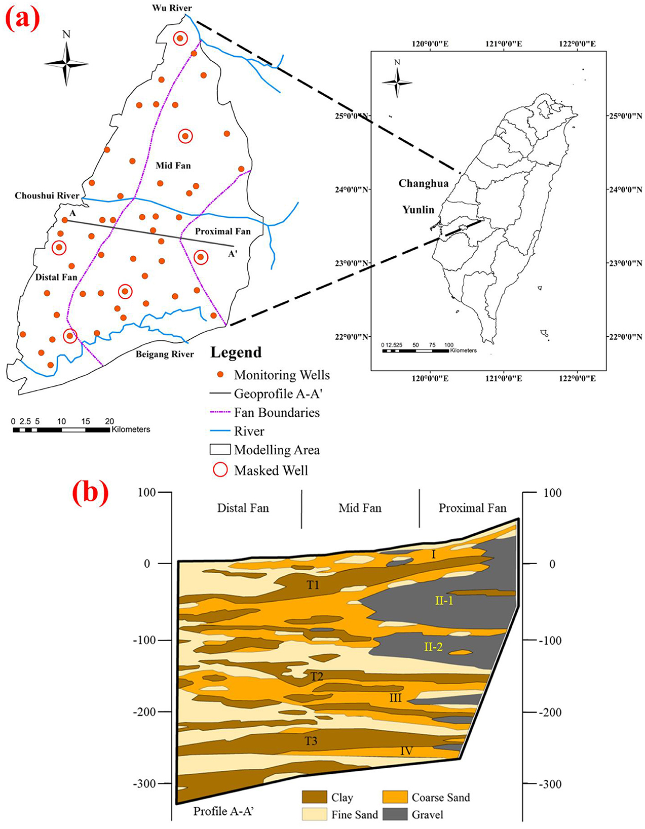
Figure 1. Choushui River Alluvial Fan (CRAF) in Central Taiwan with (a) locations of monitoring wells and (b) geological profile of the aquifer system (A–A′) (Hung et al., 2010).

2.2 Data

The hydraulic head measurements were collected from an extensive network of 51 monitoring wells spread across CRAF (Figure 1a) established by the Water Resource Agency of Taiwan. The measurements collected in this study spanned 21 years, starting from January 2001 to January 2022. These near-real-time monitoring wells measure the head changes within the aquifer system, particularly in “Aquifer-II.” The monitoring wells were selected following an initial assessment where < 5% of the data were missing. Since the primary objective of this study was to conduct monthly spatio-temporal groundwater prediction, firstly, the daily observations were transformed to monthly average values. A hydraulic head data cube (monthly image time series) was generated using the spatial interpolation technique, i.e., inverse distance weighting (Shepard, 1968). This method automatically estimates monthly hydraulic heads based on the nearby observations to appropriately generate images of 500 m × 500 m resolution having a grid size of 158 × 105 within the study area. We employed an adaptive IDW method that guarantees a set number of nearest neighbors as local samples, offering a more precise representation of spatial variability with less bias (an average absolute bias: 2.07%). This approach enabled us to generate a continuous data cube of hydraulic head, which was crucial for the modeling in this study. The method was chosen due to its demonstrated success in previous groundwater studies conducted over CRAF (Ali et al., 2020, 2021; Chu et al., 2021a,b; Tatas et al., 2022).

A total of 253 monthly uninterrupted images of hydraulic heads spanning over 21 years were prepared in this study for spatio-temporal groundwater modeling. For proper evaluation of these spatio-temporal models, the data cube of the hydraulic head was segregated into a training set that consisted of 180 images (from January 2001 to December 2015), while the remaining 73 images (from January 2016 to January 2022) were used as evaluation set, with further subdivision into validation set (2016–18) and testing set (2019–22/01).

3 Methods

Figure 2 shows the standalone CNN, LSTM, and hybrid CLSTM as image-based model structures in the context of groundwater autocorrelation modeling proposed in this study.

Figure 2

Figure 2. Groundwater model architectures of (a) CNN, (b) LSTM, and (c) CLSTM.

3.1 CNN and LSTM models

A CNN architecture was proposed in this study having one convolution layer with max pooling followed by a hidden and an output layer (see Figure 2a). CNN incorporates specific feature extraction using convolution operations to process high-dimensional datasets. CNN includes filters with varying sizes or capacities to extract any relevant features from a particular portion of the image. Filters have the capability to slide across images to extract important features from various parts of the image. The versatility of CNN involves greater control over the size, number, and movement of these convolution filters across multiple images. In this study, 2D convolution filter was utilized. Equation 1 is provided to illustrate the 2D convolution operation (Yang and Zhang, 2022):

\begin{array}{l} F (i, j) = (I * K) (i, j) = \sum_{m} \sum_{n} K (m, n) I (i + m, j + n) & (1) \end{array}

where F(i, j) is the feature map at a specific position (i, j) after convolution; K and I represent the size of the convolution filter and input image array, respectively. As the convolution filters slide across the image to extract relevant features, the corresponding feature elements are multiplied and summed. The feature map is then processed by an activation function to make it non-linear. Following the convolution process, the ReLU activation function introduces non-linearity into the network, enabling it to capture and model complex patterns and relationships. A pooling operation is conducted to downscale the feature map to preserve the most important information. Later, the downscaled 2D feature map array is flattened into a 1D vector before feeding it to a fully connected layer. Finally, the reshape function was used to transform the 1D prediction vector to a spatial image of next-month hydraulic heads (Figure 2a).

The LSTM models are critically acclaimed in various research works dealing with time series prediction, especially in the realm of groundwater (Solgi et al., 2021; Vu et al., 2021; Sun et al., 2022; Patra et al., 2023). A representation of the standalone LSTM model structure in the context of groundwater modeling proposed in this study is provided in Figure 2b. The LSTM architecture proposed in this study has one LSTM cell, a hidden and an output layer. The 2D image array was first flattened into a 1D vector before being fed to the LSTM memory cell and subsequent hidden layer. Finally, a reshape function was added to transform the output 1D vector to the original 2D array representing the spatial images of next-month hydraulic heads. Through its exclusive memory cell, LSTM has been known to handle long dependencies over large sequences (Hochreiter and Schmidhuber, 1997). This memory cell includes a gating mechanism that regulates the flow of information within a conveyor-belt-like structure known as cell state that gets updated based on the information that was kept or removed. The gating mechanism consists of a forget gate, an input gate, and an output gate, each involved in a specific task of regulating the information that is being fed within the LSTM memory cell. A brief description of the working principle of these gates is provided in the Appendix.

3.2 CLSTM hybrid model

For spatio-temporal time series prediction involving many multivariate sequences, it would be advantageous to consider the ability of CNN to extract useful spatial information, and incorporate it with a dynamic LSTM memory cell for handling temporal dependencies that would serve the purpose of accurate and reliable spatio-temporal prediction of groundwater. A hybrid integration of convolution operation with LSTM in the form of CLSTM model (Seo and Lee, 2021; Yang and Zhang, 2022) was tasked with autoregressive forecasting of monthly images of hydraulic head distribution that simultaneously considers the spatial interaction and temporal change in hydraulic head fluctuations. Through this, the model can generalize over a variety of hydraulic head sequences simultaneously, making the task of spatio-temporal groundwater modeling much more efficient. In this study, a comprehensive assessment of the CLSTM architecture is proposed in comparison to the standalone LSTM and CNN models for spatio-temporal groundwater forecasting. Additional assessments were also conducted with traditional multilayered perceptron (MLP) and RNN models (Müller et al., 2021). The primary objective of this groundwater model was to simulate the next month's (t + 1) hydraulic heads based only on the current month's (t) hydraulic head (Equation 2). This approach was finalized following a stepwise feature analysis that examined lags of up to 4 months (t, t – 1, t – 2, t – 3). By retraining sample models with the successive consideration of each lag and comparing the resulting error metrics (RMSE and r) (Figure A1), it was determined that lags beyond the current month's input (h_t) did not significantly contribute to the model's predictive accuracy.

\begin{array}{l} h_{t + 1} = f (h_{t}) & (2) \end{array}

where h_t and h_t+1 are the current and next month's hydraulic heads, respectively. The CLSTM model in this study uses a single convolution layer followed by a max pooling layer for extracting the most relevant spatial features pertaining to groundwater over CRAF. Feature maps were then flattened and given to the LSTM layer for handling the temporal change followed by a single hidden layer. Finally, an output layer alongside the reshape function was used to transform the 1D prediction vector to a spatial image of next-month hydraulic heads (see Figure 2c).

3.3 Masked CLSTM

This study further analyzes the data recovery ability of Masked CLSTM through spatio-temporal image inpainting for time-varying groundwater simulation. The model was designed to generate a complete next month (t + 1) image of the hydraulic head using the incomplete or masked current month (t) hydraulic head image as inputs. The Masked CLSTM expression can be represented by the image inpainting problem proposed here, as shown below:

\begin{array}{l} h_{t + 1}^{c} = f (h_{t}^{m}) & (3) \end{array}

where $h_{t}^{m}$ represents a masked (no-data) current month (t) hydraulic head image; $h_{t + 1}^{c}$ represents a complete next month (t + 1) image of the hydraulic head.

This Masked CLSTM was inspired by the previously proposed encoder–decoder architecture, a type of scalable vision learners trained on masked random patches of input images to reconstruct the missing pixels (He et al., 2022). In the context of Masked CLSTM, the convolution unit acts like a spatial encoder for visible subset (excluding masked tokens), which extracts spatial features from the available data. The LSTM layer plays a pivotal role of temporal decoder, reconstructing missing parts for the future hydraulic head image from latent representation and masked pixels from the input image through temporal variation (Figure 3). For this, chosen wells were completely masked (red circles in Figure 1) followed by IDW interpolation. Then, two masking scenarios were further conducted over the resulting sequence of hydraulic head images to introduce additional sporadic behavior in the incomplete dataset: (1) random point masking and (2) regional masking (Figure 4). Both scenarios evaluate the extrapolative ability of the Masked CLSTM model on incomplete temporal images and its precision to generate accurate spatio-temporal estimation. The random point masking was set at 10% through 90% (see Figures 4a–i). Here, the masking was temporally varying, i.e., each image had different location pixels that were masked out. The random masking scenario here is a preliminary case study where the masking was temporally dynamic in nature. Each hydraulic head image in the training or evaluation set had a unique masking pattern, making it more representative of a real-world scenario since intermittent sensor failures, data transmission issues, or other unpredictable events are sporadic in nature. For the regional masking, square-shaped mask windows of size (10, 10) were appended to the hydraulic head images over locations in upstream and downstream areas (Figures 4j, k) that removed the entire time series sequence for those locations. This masking scenario mimics issues when sensor or monitoring failure occurs for a prolonged period. The time series at selected wells were visualized having been masked consistently in all scenarios to assess model simulations under the masking scenarios. These masked sequence of hydraulic head images were being fed into CLSTM model for training, having the target images that included the original dataset interpolated through all groundwater monitoring wells. The parameter tuning of the Masked CLSTM model through grid search was conducted wherever necessary to evaluate their sensitivity to missing data while training and improving its accuracy. The quality of the model output, i.e., the completed image, was evaluated using root mean squared error (RMSE) and correlation coefficient (r).

Figure 3

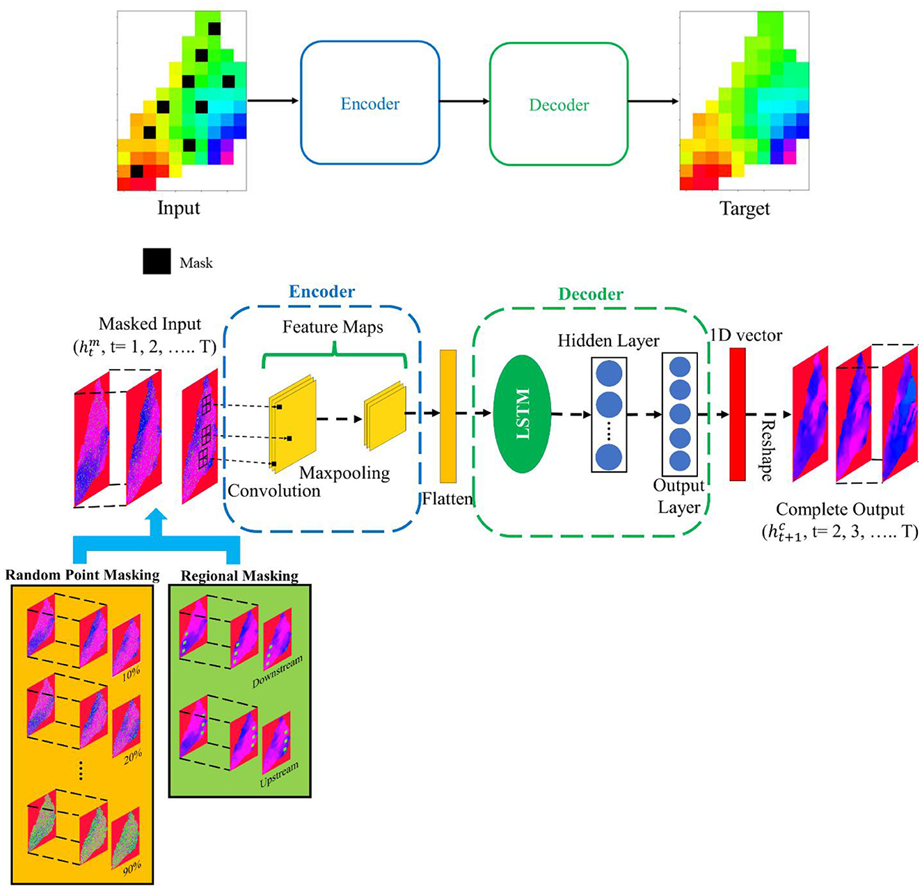
Figure 3. Spatio-temporal image inpainting in groundwater modeling using Masked CLSTM based on masked dataset scenarios such as random point masking and regional masking.

Figure 4

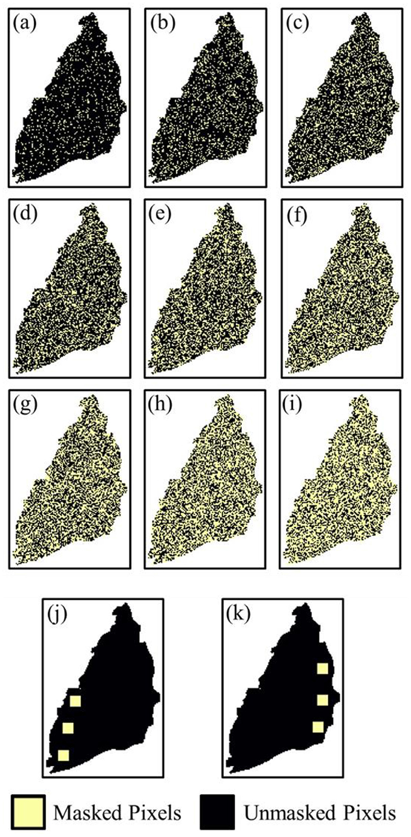
Figure 4. Randomly masked (a) 10%, (b) 20%, (c) 30%, (d) 40%, (e) 50%, (f) 60%, (g) 70%, (h) 80%, and (i) 90% for previous timestep; regionally masked (j) downstream and (k) upstream of hydraulic head images.

3.4 Data normalization, model calibration, and its assessment

The data dimensionality significantly impacts the convergence rate of deep learning models. The piezometric records from the confined aquifer over CRAF had varying ranges owing to the significant elevation change observed in the area. These piezometric readings were normalized to a common range of [0, 1] for accelerated model calibration and its convergence for accurate predictions. Normalization was applied separately to the training and evaluation datasets to prevent data leakage. The evaluation dataset (2016–22/01) was normalized using the minimum and maximum values derived from the training period (2001–15). For this study, the normalization was carried out using minimum and maximum values of a given pixel from the time series of hydraulic head images (Equation 4).

\begin{array}{l} h_{(i, j)}^{'} = \frac{h_{(i, j)} - h_{(i, j)}^{\min}}{h_{(i, j)}^{\max} - h_{(i, j)}^{\min}} & (4) \end{array}

where h_{(i, j)} and $h_{(i, j)}^{'}$ are the original and normalized hydraulic heads at a given pixel location (i, j) in the hydraulic head image. $h_{(i, j)}^{min}$ and $h_{(i, j)}^{max}$ define the minimum and maximum value obtained at the given pixel location (i, j) based on the sequence of hydraulic head images.

The model calibration was conducted over 15 years (2001–15) of the training data for 200 epochs and the corresponding assessment on the remaining 6 years (2016–22/01) of the evaluation dataset that includes both validation (2016–18) and testing (2019–22/01) sets. The objective (loss) function was set to mean squared error (MSE) with “Adam” (Kingma and Ba, 2015) as the optimizer for monitoring the status of model performance during the calibration and parameter optimization process. The training was conducted with an early stopping criterion to prevent overfitting, in which it was set to terminate when no improvement in loss function over the validation set was observed for 10 epochs. Subsequently, two standard statistical criteria, i.e., RMSE (Equation 5) and r (Equation 6) were used that adequately described the model's prediction skill for the hydraulic head. The RMSE and r values at a given pixel location (i, j) were computed from the sequence of hydraulic head images. Spatial error maps of RMSE and r were generated for each model to provide a clear visualization of the hydraulic head prediction accuracy at each location over CRAF. The models discussed in this study were generated using TensorFlow and Keras (Joseph et al., 2021) open-source libraries (Python-3.9) on a laptop configured with Nvidia GeForce RTX 3070ti GPU with 8 GB GDDR6 memory coupled with an Intel^® Core™ i9-12900H @ 3.80 Ghz CPU, 32 GB RAM, and Windows 11 home 64-bit operating system. The hyperparameter tuning of the models was carried out using a grid search approach where a set of values for each parameter was first given, and then all possible combinations were tested out, and the combinations with the lowest error were chosen as the final parameter values. The parameter tuning was mainly focused on a number of nodes and hidden layers, activation function, and number and size of convolution filter.

\begin{array}{r} R M S E_{(i, j)} = \sqrt{\frac{\sum_{k = 1}^{n} {(h_{o, k} - h_{s, k})}^{2}}{n}} & (5) \end{array}

\begin{array}{r} r_{(i, j)} = \frac{\sum_{k = 1}^{n} (h_{o, k} - {\bar{h}}_{o}) (h_{s, k} - {\bar{h}}_{s})}{\sqrt{\sum_{k = 1}^{n} {(h_{o, k} - {\bar{h}}_{o})}^{2} \sum_{j = 1}^{n} {(h_{s, k} - {\bar{h}}_{s})}^{2}}} & (6) \end{array}

Here, h_{o, k} and h_{s, k} represent the observed and simulated hydraulic head values, respectively, Similarly, ${\bar{h}}_{o}$ and ${\bar{h}}_{s}$ are the mean values of the observed and simulated hydraulic head sequence, respectively.

4 Results

4.1 Performance of CNN, LSTM, and CLSTM models

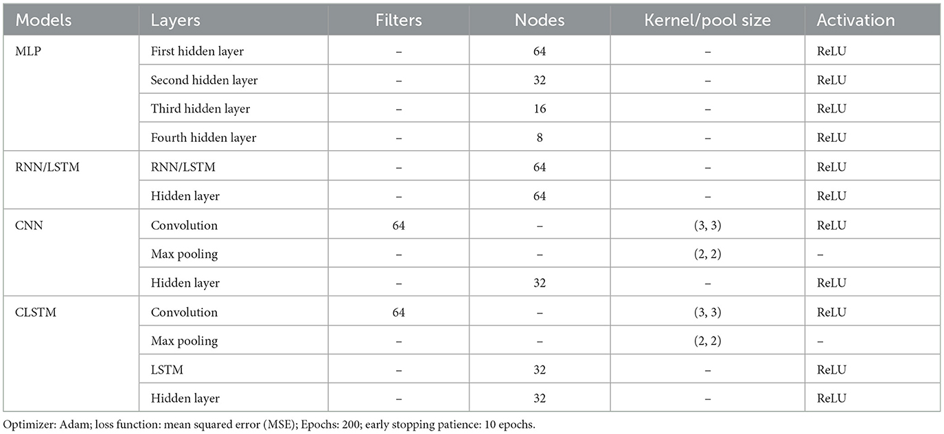
Evaluation of model performances was carried out using RMSE and correlation coefficient (r) for spatio-temporal hydraulic head prediction. Figure 5 provides the spatial error distribution maps obtained for the MLP, RNN, CNN, LSTM, and CLSTM models. For the sake of brevity, we primarily focused on analyzing model results over the evaluation dataset, which was the unseen period (2016–22/01). The relative performance of the hybrid CLSTM model showed much wider improvements across the alluvial fan in comparison to the baseline models, i.e., MLP, RNN, LSTM, and CNN. The RMSE for the next month's hydraulic head simulations dropped from almost 2 m to well below 1 m in coastal areas of Changhua County. Similarly, the r value also jumped significantly from 0.6 to over 0.85 in many locations as well here. Widespread enhancements in predictions were also observed across areas of proximal fan and mid-fan regions. RMSE values fell from 1 m to nearly 0.6 m here, while some areas close to mountains exhibited a remarkable drop of almost 50% drop. The CLSTM (RMSE ~3.3 m) model also demonstrated strong predictive skill in the southwest coastal area (drawdown-dominated) of Yunlin County in comparison to the MLP, RNN, LSTM (RMSE ~5 m), and CNN (RMSE 4–5 m) models. Consequently, r values also improved remarkably from roughly 0.8 (MLP, RNN, and LSTM) and 0.7 (CNN) to 0.95 in CLSTM model here. The nearby Central Yunlin area having severe subsidence (Ali et al., 2020; Chen et al., 2021; Chu et al., 2021b; Hung et al., 2021) witnessed noticeable improvements over several locations RNN/LSTM (~4 m) and MLP/CNN (~3 m) to (2–2.5 m) in CLSTM model. However, the uncertainties are still prevalent in this region, which could be attributed to the complexities inflicted by geological changes due to significant vertical deformation as a consequence of high groundwater abstraction. In some cases, the r values from MLP, RNN, and LSTM (Figures 5f–h) were slightly higher than the CLSTM model (Figure 5j), which indicates that these models were still able to reasonably capture the overall trend of groundwater fluctuations but had poor estimation accuracy as per RMSE over many locations. Across the alluvial fan, all models demonstrated relatively better predictive skills over the Changhua region rather than Yunlin. This area has much more extensive groundwater pumping than Changhua County, making the spatio-temporal modeling a challenging endeavor by inflicting several anthropogenic uncertainties. The RMSE values remained well within 1 m over most of the locations in Changhua, while Yunlin witnessed an RMSE value >1.5 m and sometimes even crossing 3 m from the best model, i.e., CLSTM proposed in this study. This phenomenon could be explained by high variation in groundwater in Yunlin where the standard deviation over most locations ranges between 2 and 5.5 m (variance: 10–35 m²) and is significantly higher with respect to Changhua County (0–2.5 m). Currently, groundwater exploitation may not be a serious issue in Changhua, which could be the primary reason for such low groundwater variation and low RMSE values obtained here. However, the CLSTM model can reasonably simulate the groundwater changes across the alluvial fan simultaneously with respect to baseline models for better water resource planning of the whole groundwater basin, which are interconnected with one another to some extent. Additionally, the optimal parameters for the models are given in Table 1.

Figure 5

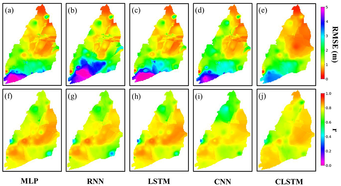
Figure 5. Spatial maps of RMSE (a–e) and r (f–j) obtained during the evaluation period (2016–22/01) from MLP, RNN, LSTM, CNN, and CLSTM models.

Table 1

Table 1. Optimal parameters for MLP, RNN, LSTM, CNN, and CLSTM models.

For the sake of brevity, the comparative analysis of the CLSTM model from here on is mainly emphasized with CNN and LSTM, as the performance of RNN was drastically poorer than LSTM, whereas the MLP consistently underperformed compared to the CNN, especially in terms of RMSE. The time series plots are depicted in Figure 6 for the three models (CNN, LSTM, and CLSTM) over six arbitrarily chosen wells spread across CRAF. It is clearly observed that the peaks and troughs simulated by the CLSTM model were the best reflections of the observations. The residual plots for the evaluation set from CLSTM model nearly followed a normal distribution (see Figure 7c) due to their strong spatio-temporal contextual learning ability, and a slight skewness was witnessed for both LSTM and CNN (Figures 7a, b). While the LSTM model showed slightly better r values in comparison to CNN and CLSTM models, through the graphical visualization, it can be inferred that the CLSTM model adequately captured the seasonal variability of the groundwater system and provided the best estimation. This can also be further evidenced through the simulated spatial distribution of hydraulic heads illustrated in Figure 8, representing the recent winter (January 2021), summer (July 2021), and fall seasons (October 2021). The summer and fall periods are usually dominated by frequent downpours in Taiwan. The spatial distribution of hydraulic heads simulated by the CLSTM model was more accurate in representing the spatial distribution of next-month groundwater condition. Overestimations were witnessed in the summer season (July 2021) from the standalone LSTM and CNN models in the southwest coastal area (drawdown-dominated) of Yunlin County, as was evident from the RMSE maps. Furthermore, stepwise feature assessment on lags of up to 4 months indicated that the current month (h_t) input (Figures 5e, j) was the best feature in driving the precision of model estimations, where its removal considerably increased RMSE (>5 m) and decreased r (< 0.1) (Figure A1) across the region. In addition to this, the proposed CLSTM model outperformed and showed widespread improvements in RMSE and r in comparison to other traditional models such as MLP and RNN (Figures 5a, b, f, g). Additional evaluation was also conducted by modifying the periods considered in training (2007–22/01) and evaluation (2001–2006) sets for model training. The spatial error maps for the evaluation set during 2016–22/01 (Figure 5) or 2001–2006 (Figure A2) are mostly identical, and CLSTM model manages to outperform the standalone CNN and LSTM models. This shows the superiority of CLSTM while dealing with image time series prediction of groundwater that combines the relevant spatial features extracted by the convolution filter together with the power of LSTM memory cell to simultaneously handle various temporal dependencies, thereby improving the adaptability and robustness of the combined model. Moreover, it is worth pointing out that the CLSTM model was trained only using the past observation of hydraulic head which could be a reliable surrogate for the regional variability of rainfall and anthropogenic activities. This makes the model proposed in this research more applicable over a wider range of groundwater basins for near-real-time groundwater monitoring and management through reliable spatio-temporal forecasts of monthly hydraulic heads when adequate availability of meteorological variables is relatively scarce. The learning curves associated with the three models' training are provided in Figure A3 of the Appendix section. The learning curves reveal important insights into the training process and performance of the models. The LSTM model (Figure A3a) shows considerable fluctuation in both training and validation loss, particularly in the initial epochs, indicating challenges in stabilizing and generalizing to spatial heterogeneity associated with regional groundwater variation. The CNN model (Figure A3b) demonstrates a rapid reduction in training loss, suggesting efficient learning of spatial features. However, the greater variation in validation loss highlights potential issues with temporal generalization. In contrast, the CLSTM model (Figure A3c) exhibits a rapid and stable reduction in both training and validation loss, reflecting its ability to effectively capture both spatial and temporal dependencies. The close alignment of training and validation losses for the CLSTM model underscores its robust generalization capabilities, making it better suited for regional modeling tasks compared to standalone CNN and LSTM models. The spatial maps of RMSE and correlation coefficient (r) obtained for the training subset through CNN, LSTM, and CLSTM models are given in Figure A4.

Figure 6

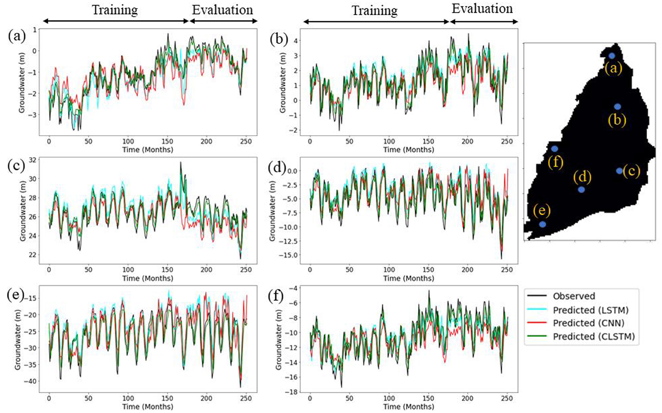
Figure 6. Time series plots of the simulated groundwater by LSTM, CNN, and CLSTM models over six distinct wells (a–f) during training (2001–15) and evaluation (2016–22/01) periods.

Figure 7

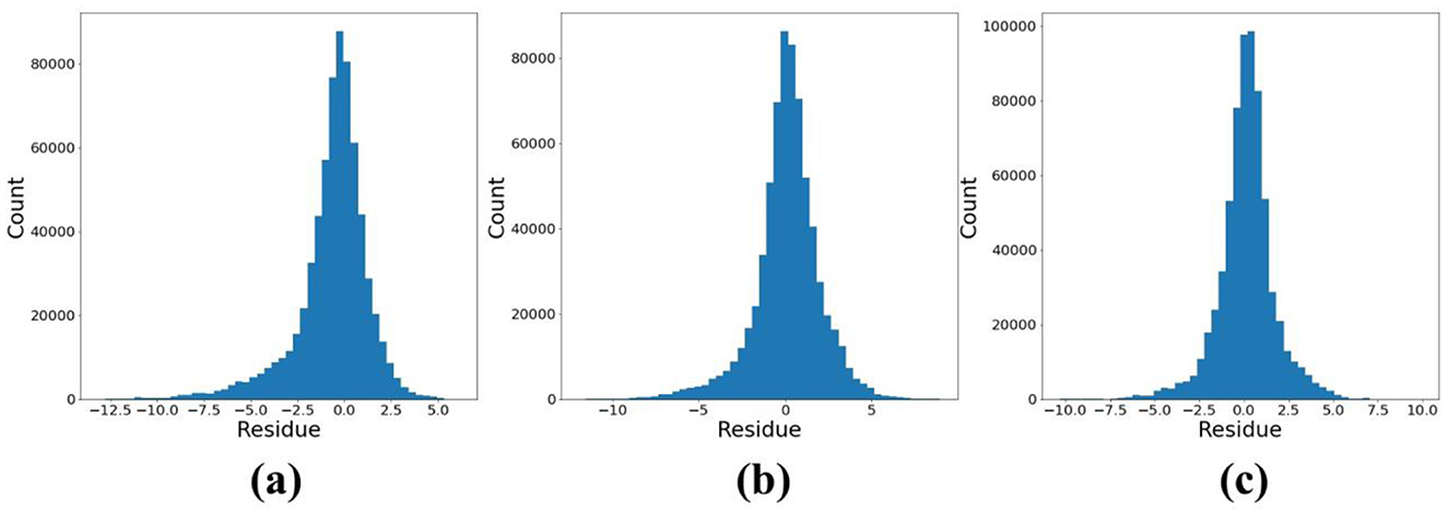
Figure 7. Distribution of model residue obtained for the evaluation period (2016–22/01): (a) LSTM, (b) CNN, and (c) CLSTM (unit: m).

Figure 8

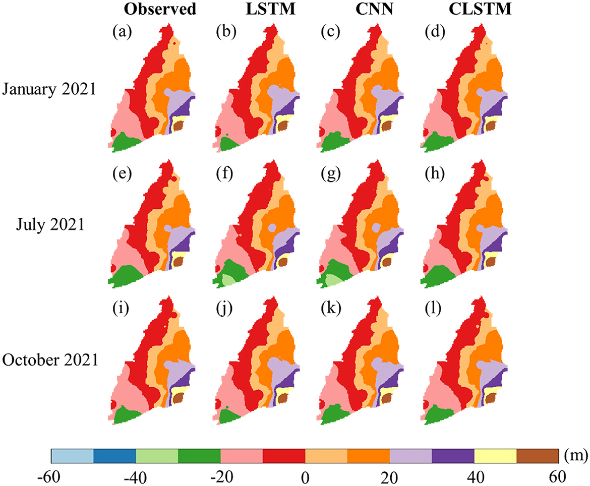
Figure 8. Observed vs. simulated spatial distribution of hydraulic head from LSTM, CNN, and CLSTM models in January (a–d), July (e–h), and October (i–l) of 2021.

4.2 Spatio-temporal reconstruction in groundwater forecasting

The Masked CLSTM model was also proposed and evaluated under various masking scenarios in simulating complete spatial images of monthly hydraulic heads. The spatial maps for RMSE and r obtained for all random point masking scenarios over the evaluation set are depicted in Figures 9, 10, respectively. All obtained error maps having 10–90% masked pixels are somewhat identical to the error distributions witnessed under the no masking condition (Figures 5e, j). However, the model performance starts to slowly deplete, beginning at 60% masking, especially in terms of r (Figure 10f) with the most prominent errors observed for 80% (Figures 9h, 10h) and 90% (Figures 9i, 10i). Still, the Masked CLSTM model showed greater data recovery capability with 80% and 90% missing pixels where over 90% of the data were adequately recovered, which is evident from their error distribution maps (see Figures 9h, i, 10h, i). The (3, 3) sized convolution filter developed in this study could still learn the contextual information even after several missing pixels, which is indicative of the superiority demonstrated by such advanced CNN-based deep learning technique in the field of groundwater modeling. The time series plots observed for six masked wells (red circle in Figure 1) are also indicative of the high level of spatio-temporal extrapolative ability of the Masked CLSTM model (Figure A5). For all scenarios, the simulated hydraulic head values were much closer to the originally recorded fluctuations. However, at 80 and 90% masking, as previously indicated, the model predictions slightly deviated more from the observation values at some locations. The peaks and troughs were occasionally under-predicted due to significant information loss. Still, the model showed potential signs of adequate learning capabilities under masked scenarios by authentically capturing the overall seasonal variability of the masked locations, which is a sign of reliability over its simulated groundwater conditions when significant dataset is limited. The results reported in this section for random point masking were based on the same model parameter values of CLSTM given in Table 1.

Figure 9

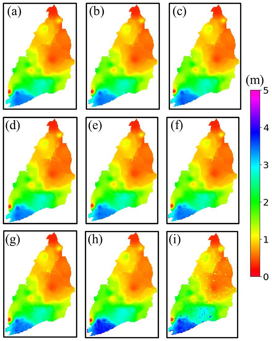
Figure 9. RMSE maps for the random point masking scenario in the evaluation set (2016–22/01) in Masked CLSTM considering (a) 10%, (b) 20%, (c) 30%, (d) 40%, (e) 50%, (f) 60%, (g) 70%, (h) 80%, and (i) 90% masking.

Figure 10

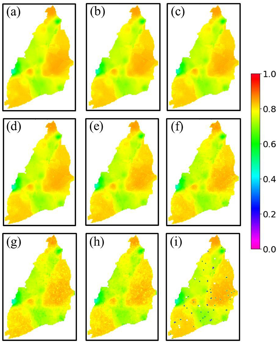
Figure 10. Correlation coefficient (r) maps of the random point masking scenario in the evaluation set (2016–22/01) in Masked CLSTM: (a) 10%, (b) 20%, (c) 30%, (d) 40%, (e) 50%, (f) 60%, (g) 70%, (h) 80%, and (i) 90% masking.

For the regional masking scenario, the downstream region that was selected from the Yunlin area is primarily used for aquaculture activities, which induces various uncertainties in the hydraulic head records. The upstream side is a major recharge zone where most of the groundwater recharge occurs, thereby heavy influence from natural hydrological cycles. The model under two distinct hydrological conditions satisfactorily provides good data recovery opportunities. The error maps (Figure 11) obtained under two regions, specifically the masked areas (black squares), retained relatively close RMSE and r values over most of the masked pixels compared to the results with no masking (Figures 5e, j). However, some parts of the upstream side that were masked (central) witnessed a slight increase in RMSE (Figure 11b). The simulated sequences (Figures A6, A7) observed for both cases within the masked region indicate that the model reasonably predicts the hydraulic head in the masked coastal parts and the upstream. There is less variance in the hydraulic head records in the upstream area having limited pumping and reduced anthropogenic interference. In contrast, the coastal side that was masked for this case study is vastly covered with anthropogenic pumping for aquaculture and several other uncertainties induced by the infiltration from nearby fish ponds or leakage through the pumping wells (Liu et al., 2003). However, the model adequately captures the overall variability in the hydraulic head fluctuations and can potentially provide reliable groundwater simulations under data-limited conditions. It is important to point out that the most influential hyperparameter of the model sensitive to masking size, especially for the regional scenario, was found to be the kernel size for convolution operation. The square mask size was fixed at 10 × 10 pixels; therefore, the model's image inpainting performance worsened with any kernel size value lesser than (10, 10). The results reported in this section for the regional masking scenario were achieved using the kernel size of (11, 11), while the remaining parameters were left unchanged (Table 1). As a whole, the masking experiments conducted in this study provide evidence of an overarching advantage of incorporating the Masked CLSTM approach for simulating reliable groundwater conditions at locations with sensory errors or power outages and thereby contributing to its effective monitoring.

Figure 11

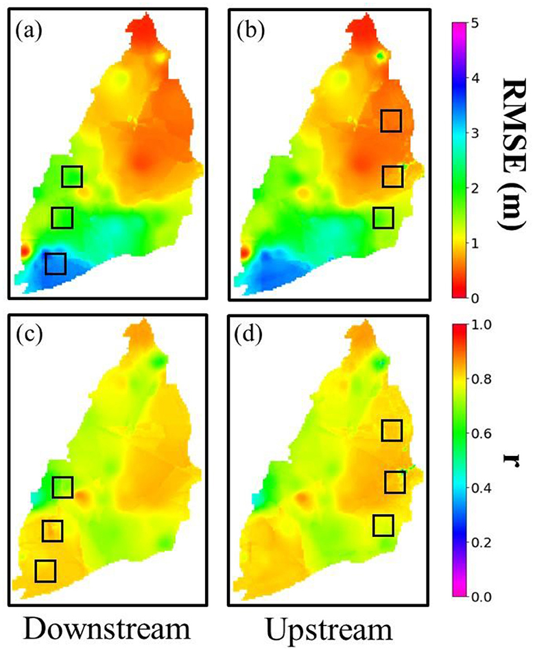
Figure 11. Spatial maps of RMSE (a, b) and r (c, d) in the evaluation set (2016–22/01) (note: black squares are the regionally masked areas) in Masked CLSTM for regional masking scenarios at downstream and upstream.

5 Discussion

5.1 CLSTM for spatio-temporal groundwater modeling

The study highlights the effectiveness of the CLSTM hybrid architecture as a superior alternative to the baseline LSTM and CNN models in groundwater modeling. By extracting relevant features through convolution filters and downsampling via max pooling, the trained LSTM layer demonstrated the ability to generalize across images, resulting in more accurate forecasts of the future state of groundwater. The CLSTM model outperformed the standalone LSTM model that is widely adopted for time series prediction tasks. The standalone LSTM and CNN models demonstrated extremely poor results in the drawdown-dominated southwest coast, with RMSE almost touching 5 m and r values 0.6–0.7, whereas the CLSTM model reduced RMSE 3.2 m and achieved better r value of about 0.9. The southwest coastal region is characterized by significant groundwater drawdown due to extensive pumping, leading to complex and high variance in groundwater levels. Standalone CNN and LSTM models, which might excel in capturing spatial or temporal patterns individually, struggle to accurately model these interactions. CNNs are primarily designed to capture spatial features but lack the capability to effectively model temporal dependencies, which are crucial in regions with significant drawdown and variable groundwater extraction rates. LSTMs are effective at capturing temporal sequences but are not inherently designed to model complex spatial heterogeneity, such as varying subsurface conditions or localized pumping effects. This spatial heterogeneity is particularly pronounced in drawdown-dominated regions, leading to suboptimal performance when using LSTM alone. These limitations resulted in poorer performance from standalone models in regions where simultaneous consideration of spatial and temporal dynamics is critical. Moreover, these models showed poor performance in northern parts of Changhua and nearby coast, where the improvement in RMSE and r was observed around 20%−50% from CLSTM model. Interestingly, the number of nodes for the LSTM layer and the subsequent hidden layer reduced from 64 to 32 in CLSTM when compared to the standalone LSTM model (see Table 1). Such a considerable decrease in node requirements can be attributed to the decreased complexity of the LSTM layer after convolution and max pooling operations since subsequent layers are only trained on downscaled but essential features. A standalone LSTM model mostly performs inefficiently for such tasks since it was not designed to handle large multiple time series sequences simultaneously while considering their interdependencies. In addition, the CLSTM converged faster and required relatively less epoch to learn the spatio-temporal dependencies, making it the most efficient model in our study. This model also addresses one of the potential limitations in the Local-LSTM models that were previously proposed (Patra et al., 2023), each trained on single local well data over the same study region. However, the trained Local-LSTM model was designed to make groundwater forecasts on the remaining monitoring wells in the region, which made its performance vulnerable to abrupt changes in temporal characteristics over far away, located wells that could make its estimation highly uncertain. This dilemma can be effectively resolved by incorporating a prior convolution layer with LSTM, i.e., CLSTM, enabling it to be trained simultaneously on all locations at once and can effectively handle and generalize across diverse sets of hydraulic head records with varying temporal characteristics that are usually attributed to changes concurrently within a single model. As demonstrated in this research, the CLSTM model outperformed standalone as well as traditional models, which is in alignment with the past claims demonstrated by closely related research works. For instance, Seo and Lee (2021) reported a 10%−12% improvement in RMSE and r with respect to standalone LSTM for predicting groundwater storage change in South Korea. Similarly, Yang and Zhang (2022) noted that their hybrid integration of CNN and LSTM approach yielded a significant increase in prediction accuracy, reducing error rates by almost 33.6% in comparison to LSTM and other traditional models for predicting groundwater level in middle and lower reaches of the Heihe River, China. Further improvement in spatio-temporal groundwater prediction can be achieved by incorporating data from various sources, such as hydrometeorology and human activities (pumping), if adequately available, that can in turn be used to further generate groundwater projections for the long-term under climate change scenarios.

5.2 Masked CLSTM in groundwater modeling

Similar to the Masked Autoencoder (He et al., 2022), the Masked CLSTM can operate as a spatio-temporal visual learner that includes a convolution layer acting as spatial encoder extracting useful features from the subset of hydraulic head images, such as the patterns, gradients, and edges, that are crucial for filling the missing pixels. This enables the following LSTM layer, which is the temporal decoder of essential spatial features within the hydraulic head fluctuations over time, such as trends, seasonal variations, cycles, and long-term dependencies. The synergistic integration of these layers drastically increased the adaptability of the resulting model, allowing it to infer dynamically missing information based on learned spatio-temporal dependencies or self-similarity of groundwater levels. Even with 80% of the masked pixel, the model achieved good performance, and the resulting error map closely resembled the results obtained without any masking. Although the data recovery from the model still starts to be slightly affected from 60% masking while severe gaps were observed at 90%. The model successfully recovered and predicted the hydraulic head values when a considerable portion of pixels was regionally obscured as a square shape in the upstream and the downstream coastal areas. The primary reason for Masked CLSTM in achieving such reasonable performance was due to its effective learning of spatial and temporal dependencies in spatio-temporal image inpainting. The kernel size of the convolution filter is one of the most influential parameters for spatio-temporal image inpainting in this case. A larger kernel size enables the model to learn more spatial contextual information for filling up larger pixel gaps in the image, as observed in regional masking scenario.

The investigations illustrated in this study imply toward the potential implementation of an AI-based image inpainting approach in groundwater monitoring and management, particularly on the inputs from sensors that are seldomly obscured by power outages or sensor errors leading to the unavailability of spatial signatures. This approach can be further integrated into (1) operationalization of incomplete datasets where water resource monitoring agencies/industry could benefit from this research, thereby operationalizing these models that handle incomplete data effectively which can lead to more efficient use of available information, and (2) mitigation pertaining to data collection challenges that usually involve time-consuming field work, costly equipment, and inaccessible locations. The model can provide reasonable estimates in the absence of certain information and can be instrumental in mitigating these challenges and making predictions possible with partial datasets. Previous studies (Seo and Lee, 2021; Yang and Zhang, 2022; Moudgil and Rao, 2023) have not yet explored the possibility of applying a deep learning-based image inpainting in hydrological modeling, specifically for groundwater studies. Our study would greatly benefit the groundwater field, which heavily relies on field data, which may offer a promising alternative to handle data quality/availability issues and contribute to more reliable information on locations with missing data. This study can provide innovative AI-driven model to critical issues such as data inconsistencies that continue to plague the groundwater field. Nevertheless, findings discussed in this work for image inpainting are an indicator of high superiority and versatility in advanced deep learning models for demonstrating powerful learning, adaptability, and generalization capabilities under various masking scenarios. The CLSTM model's robustness is evident in its performance across various regions of the Choushui River Alluvial Fan, which is characterized by a wide range of geological and climatic conditions. The model has shown strong predictive capabilities in both high groundwater abstraction areas (e.g., Central Yunlin) and regions with less severe exploitation (e.g., Changhua County). The ability of the CLSTM to generalize well across these diverse conditions suggests that it effectively captures the underlying spatio-temporal patterns governing groundwater dynamics where certain regions or time periods had missing data. This would lead to a real-time Masked CLSTM model in capturing the inter-variable dependencies under complex scenarios when the locations and the shapes of the masks change temporally.

6 Conclusion

An effective CLSTM architecture was presented for spatio-temporal prediction of groundwater variations and was then assessed against the conventional LSTM and CNN models as well as MLP and RNN. The hybrid model contains great forecasting capabilities in temporal groundwater changes from LSTM and captures spatial features of groundwater patterns using CNN. The statistical evaluation of the simulations generated by these models involved the use of RMSE and correlation coefficients across the evaluation dataset. Results revealed that the CLSTM model significantly outperforms MLP, RNN, CNN, and LSTM models in most cases. This spatial feature extraction allows the model to retain essential spatial information and combine it with the temporal dynamics processed by the LSTM layer. The model achieved better simulations over most of the locations within upstream and southwest pumping-dominated coastal regions of CRAF while showing commendable improvements in the coastal regions of Northern Changhua and its nearby coastal area. Moreover, Masked CLSTM promoted a reliable assessment of the spatial distribution of hydraulic heads simulated to make a well-informed decision on the most appropriate approach for subsequent image inpainting experiments. Consequently, the Masked CLSTM was tasked to solve the spatio-temporal reconstruction problem using image inpainting for groundwater prediction. This model demonstrated greater capabilities in recovering the data under various masking scenarios and provided acceptable results from the lagged hydraulic head images with missing pixels, especially with 80% masking. Results are indicative of the advantages and potential of adopting Masked CLSTM beyond only groundwater prediction on historical datasets to recover groundwater information over locations that suffer from sensory errors or power outage issues.

This study provides a sophisticated study on the CLSTM model for reliable and efficient groundwater forecasting over a wider spatial extent, even with partial data. This study is an essential step toward effective groundwater resource planning and sustainable management that substantially contributes to mitigate groundwater depletion. Future studies can strive to explore the effects or sensitivity to missing data over the data recovery capabilities of the Masked CLSTM model with image inpainting on groundwater modeling over other regions. Moreover, future studies could expand upon the use of other iterations of hybrid/generative AI models such as transformers, generative adversarial networks, and graph neural networks for groundwater modeling or assessing the impacts of climate change on groundwater by considering more hydrometeorological data into the models.

Data availability statement

The raw data supporting the conclusions of this article will be made available by the authors, without undue reservation.

Author contributions

SP: Data Curation, Formal Analysis, Investigation, Validation, Visualization, Conceptualization, Methodology, Writing – original draft. H-JC: Data Curation, Funding Acquisition, Investigation, Resources, Conceptualization, Supervision, Writing – review & editing.

Funding

The author(s) declare financial support was received for the research, authorship, and/or publication of this article. This study was supported by National Science and Technology Council (NSTC), Taiwan and Miin Wu School of Computing, NCKU.

Acknowledgments

The authors would like to thank the editors and reviewers for providing suggestions for paper improvement. Furthermore, the study was supported by the National Science and Technology Council (NSTC), NCKU Miin Wu School of Computing, and Water Resources Agency, Taiwan.

Conflict of interest

The authors declare that the research was conducted in the absence of any commercial or financial relationships that could be construed as a potential conflict of interest.

Publisher's note

All claims expressed in this article are solely those of the authors and do not necessarily represent those of their affiliated organizations, or those of the publisher, the editors and the reviewers. Any product that may be evaluated in this article, or claim that may be made by its manufacturer, is not guaranteed or endorsed by the publisher.

Supplementary material

The Supplementary Material for this article can be found online at: https://www.frontiersin.org/articles/10.3389/frwa.2024.1471258/full#supplementary-material

References

Ali, M. Z., Chu, H. J., and Burbey, T. J. (2020). Mapping and predicting subsidence from spatio-temporal regression models of groundwater-drawdown and subsidence observations. Hydrogeol. J. 28, 2865–2876. doi: 10.1007/s10040-020-02211-0