Reconstructing 169 years of historical atmospheric and hydrologic conditions in the American River Watershed through the Watershed Environmental Hydrology Hydro-Climate Model system

The risk of more frequent and intensified extreme events is expected to increase with climate change. In semi-arid regions, particularly, both increased flooding and prolonged droughts pose a threat as the water resources system must be prepared for both types of extremes. To understand how future extremes may be altered, however, past extremes must be understood. For this reason, this study employs three physically based models to simulate the atmospheric, snow, and hydrologic conditions in the American River Watershed: the Weather Research and Forecasting Model and the Watershed Environmental Hydrology Hydro-Climate Model with the addition of a SNOW Module. Each model is individually calibrated and validated against either gauge data or data provided by the Parameter-Elevation Regressions on Independent Slopes Model for two 10-year periods before a full 169-year daily reconstruction is performed for the period from 1852 through 2020. To analyze the model performance under hydrologic extremes, three flood years (1997, 2006, and 2017) and two drought periods (1987–1992 and 2012–2016) are further analyzed. The reconstruction outputs are found to successfully simulate historical conditions at both daily and monthly scales. Results highlight the importance of fully accounting for the role of temperature in snow processes and the subsequent flow conditions. By understanding how the models perform under historical extreme conditions, future extreme events can be compared, and necessary adaptation plans can be conceived to ensure that the watershed is prepared for future wet and dry conditions. Additionally, the created reconstruction dataset is comprehensive, simulating conditions across the hydroclimate, at a finer spatial and temporal scale than is typically available from observation data alone. The dataset can be further analyzed to assess changes in the trends and the potential trajectory of extreme events within the American River Watershed.

1 Introduction

Climate change is widely accepted to be impacting global atmospheric mechanisms and contributing to changes that alter the hydrologic response to atmospheric conditions (Young et al., 2009; Singh et al., 2018; Moustakis et al., 2021; Welty and Zeng, 2021; Lee et al., 2023). Preparing the current water management system to be flexible and adaptable to the consequences of climate change is vital, especially in regions where the occurrence of extreme events is expected to increase (Facincani Dourado et al., 2024). While the definition of an extreme event is location-specific and likely to change as severe storms become more common, understanding past atmospheric and hydrologic conditions for an area is important before attempting to understand how these characteristics may change in the future (Ishida and Kavvas, 2017; Pendergrass, 2018). As such, this study aims to reconstruct historical atmospheric, snow, and hydrologic conditions using three physically based models. Daily simulations for the period from 1852 to 2020 are conducted for the American River Watershed (ARW) using the Weather Research and Forecasting (WRF) model and the SNOW Module and hydrologic components of the Watershed Environmental Hydrology Hydro-Climate Model (WEHY-HCM). Following the calibration and validation of each of the three physically based models, overall output performance is compared to historical observations. With the reconstruction dataset, important extreme events, for precipitation, flooding, and drought, can be further analyzed and model performance assessed.

The target watershed for the application of the proposed methodology is the American River Watershed (ARW). Located in the Sierra Nevada Mountain range to the east of Sacramento, California, ARW drains ~5,440 km² into Folsom Reservoir at the outlet of the watershed through three main river forks. Operational in 1956, as part of the Central Valley Project, Folsom Reservoir has a total capacity of ~1.2 billion m³, providing both flood protection and water supply to the Sacramento area (Bureau of Reclamation). As a heterogenous, mountainous watershed, the elevation within ARW ranges from 120 m near Folsom Reservoir to close to 3,000 m in the headwaters of the Sierra Nevada (Figure 1A). The higher elevations in the headwaters provide important snow cover and contribute spring and summer snowmelt to streamflows when precipitation is not typically available. Land use and land cover (LULC) over the watershed is primarily forest with the low elevations near Folsom Reservoir, and extending up the mountain along the stream reaches, consisting mostly of deciduous broadleaf forest (Figure 1B; California Department of Forestry and Fire Protection, 2015). Around Folsom also contains shrubland and grassland, in addition to concentrated zones of urban areas and irrigated cropland. At mid elevations, between 1,000 and 2,200 m, coverage is mostly evergreen needleleaf forest with some pockets of shrubland and deciduous broadleaf forest along the high slope stream reaches (Figure 1C). Finally in the highest elevations, above 2,500 m, the mountain tops are barren or sparsely vegetated.

Figure 1

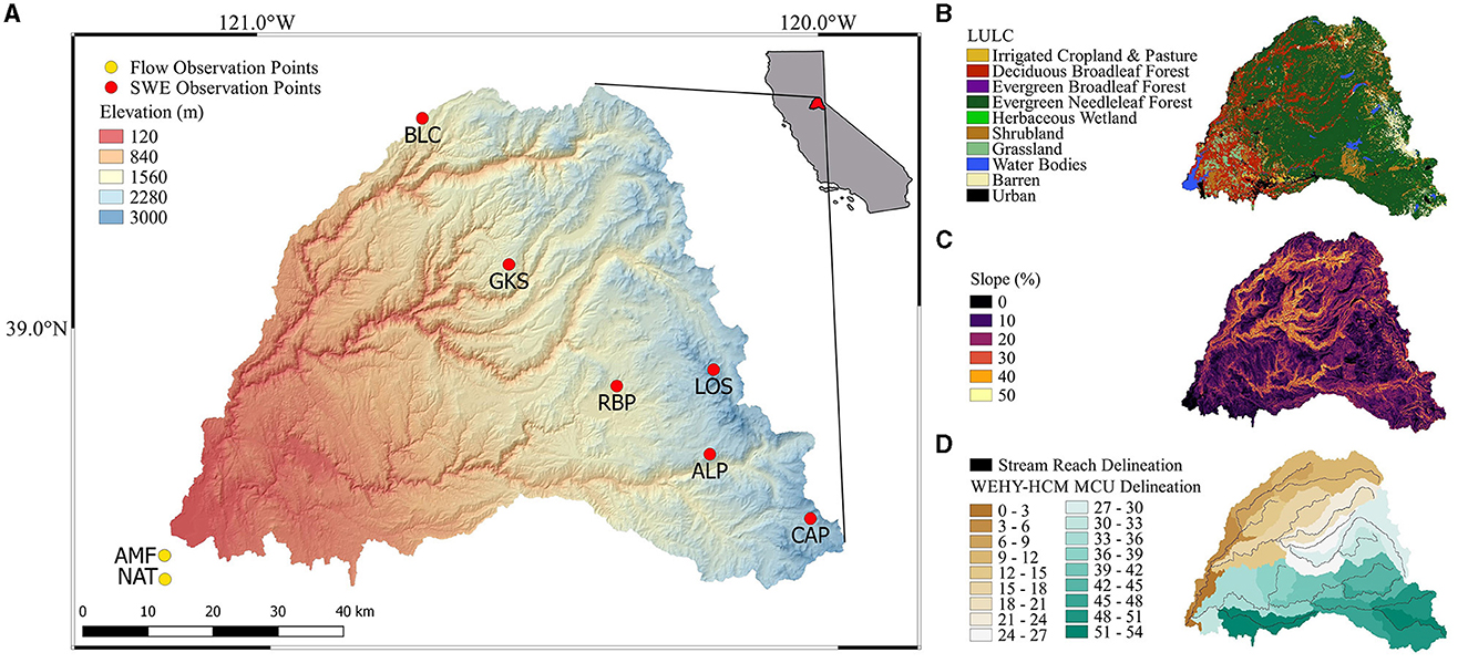
Figure 1. Characteristics of the American River watershed including (A) the location within CA and the elevation, (B) land use and land cover, (C) slope, (D) WEHY model computational unit and stream reach delineation.

ARW climatology can be characterized as a modified Mediterranean climate, with essentially a wet season and a dry season (National Research Council et al., 1999; Swain et al., 2018). The wet season, typically October through March of a water year, is defined by precipitation building through the late fall before peaking in the winter months and subsiding into the early spring. Similarly, snowpack will peak around the end of March with melting occurring from April through July following the rise in temperature. The dry season, typically April through September, is defined by rare late spring precipitation declining through the summer and early fall.

Flooding will generally occur in the wet season, coinciding with precipitation events, and often as a result of persistent onshore atmospheric flow patterns, namely atmospheric rivers (Dettinger, 2011; Ishida et al., 2015; Ralph et al., 2019). Though the landfall location of an atmospheric river can create variability in the precipitation that a given watershed will receive, both the antecedent soil conditions and local topography are crucial in the hydrologic response that will follow (National Research Council et al., 1999; Chen et al., 2018; Swain et al., 2018). Soil moisture is a key land condition controlling the hydrologic response to a precipitation event, as an already saturated watershed can significantly increase streamflow as all precipitation is converted to runoff (Ohara et al., 2011; Ralph et al., 2013). Orographic precipitation is another critical mechanism in the Sierra Nevada range, and particularly ARW, as the incoming high-moisture flows are forced upward when they collide with the mountain range, causing the moisture to precipitate out (Ohara et al., 2011; Moustakis et al., 2021). Under certain conditions, such as a rain-on-snow (ROS) event, flooding is possible as warm precipitation falls on a persistent snowpack, contributing to increased streamflow beyond the precipitation rate alone (Welty and Zeng, 2021).

In terms of a changing climate, intensifying precipitation and drought are of particular concern, as the potential increase in whiplash events between extreme wet and extreme dry conditions make managing competing water demands more difficult (Swain et al., 2018; Facincani Dourado et al., 2024). As with many California watersheds, an increase in the frequency of extreme precipitation, in conjunction with aging infrastructure, increases the potential hazard for the loss of life and property damage in communities downstream of large reservoirs, such as Folsom, should dam failure or levee breaches occur (Concha Larrauri et al., 2023). The effects of a warmer atmosphere also have implications for snow processes, which often control spring and summer runoff (Dettinger et al., 2004). Snow accumulation may be relegated to high elevations, where air temperatures still get cold enough for precipitation to fall as snow (Trinh et al., 2017; Ishida et al., 2018). Warmer temperatures may ultimately change the frequency and timing of ROS events depending on the elevation and snow distribution (Clavet-Gaumont et al., 2017; Singh et al., 2018; Li et al., 2019). At elevations above ~2,000 m, a risk for an increase in the frequency of ROS events is predicted, should warmer atmospheric flows quickly melt any previously accumulated snowpack. However, below this approximate elevation, ROS events may decrease as warmer temperatures lead to diminished snowpack. Beyond flooding, the risk of long-term droughts is also present with both societal and economic consequences, should multiyear periods of below average precipitation occur (Abatzoglou and Williams, 2016; Swain et al., 2018; Konapala and Mishra, 2020).

Even if extreme wet and dry periods are expected to increase, it is possible that on average the expected yearly volume of streamflow may not change much into the future (Dettinger et al., 2004). Temperature alone does not directly control runoff changes, and in a complex non-linear system, there is still inconsistency in future streamflow trends depending on the projections and models used as well as variation across regions and seasonality (Tang and Lettenmaier, 2012; Elbaum et al., 2022; Douville, 2024). However, even slight changes to the timing of streamflow can impact current reservoir operations which have to balance flood control and drought storage (Dettinger et al., 2004). Larger increased winter streamflow from increased liquid precipitation can lead to higher reservoir releases for maintaining flood control space but results in less water available for spring and summer water supply and riverine ecosystem needs. Though much uncertainty remains in how exactly future extreme events will change, in terms of sustainable water resources management and dam operations, decision-makers need to be prepared for the variety of changes and risks that are hypothesized, to be able to maintain adequate flood protection while also preserving storage for downstream demand during drought periods (Facincani Dourado et al., 2024). Preparing for hydrologic changes in response to a changing climate is a complex problem that must be taken at an individual basin-scale to account for the spatial heterogeneity and non-linearity of the system (Li et al., 2019; Douville, 2024). Studies at a global scale can assess trends for regions, however, the impact of LULC and water management changes at a basin-scale cannot always be accounted for. Additionally, as mitigation and adaptation plans are assessed and implemented at state and local levels, without long term, complete historical records, it is difficult to distinguish between natural hydrologic variability and changes due to warming (Dettinger et al., 2004; Facincani Dourado et al., 2024). By utilizing physically based atmospheric and hydrologic models in this study, the rare combination of precipitation, temperature, snow processes, and streamflow within a watershed that can lead to either extreme flooding or drought can be simulated. Through reconstructing the 169 years of historical atmospheric and hydrologic conditions at a daily and monthly scale, this study is a first step in understanding and contextualizing estimates for future extreme events and assessing adaptation strategies. The high spatial and temporal resolution of the created reconstruction dataset can be used to constrain climate projection outputs, such as unrealistic basin-averaged precipitation values, in addition to providing a long-term dataset to test various adaptation plans that may be assessed for the Sacramento River system (Douville et al., 2022; Facincani Dourado et al., 2024). The goal of this study is to create a comprehensive, physically based reconstruction of the entire hydroclimate system for ARW, which can provide a basis for understanding the past and present conditions in the watershed to compare against projected impacts under a changing climate.

2 Materials and methods

To simulate the mechanisms that contribute to various types of extreme events, it is necessary to fully account for the non-linear processes and feedback loops that occur in and between the atmosphere and land systems (Kavvas et al., 1998). Heat and moisture fluxes, in particular, impact atmospheric dynamics and land surface conditions. Their inclusion, or not, in models of atmospheric and hydrologic processes significantly impact the conclusions that are ultimately drawn from results. Additionally, the heterogeneous, mountainous characteristics of ARW require fine scale, physical modeling of both atmospheric and land surface processes.

As such, to reconstruct the historical atmospheric and hydrologic conditions in ARW, three physical models are used. For the atmospheric reconstruction, the Weather Research and Forecasting (WRF) model is utilized to perform dynamical downscaling of global reanalysis data. For the hydrologic conditions, the physically based land hydrologic components of the Watershed Environmental Hydrology Hydro-Climate Model (WEHY-HCM) are used. The SNOW Module of WEHY-HCM is also necessary, to fully account for the role of snow accumulation and melt processes in the generation of flow discharge across the watershed. Each of these three models are individually calibrated and validated against observation data, where available. The proposed procedure to complete the ARW atmospheric and hydrologic reconstruction is as follows:

1. Calibrate and validate the WRF model for two independent 10-year periods;

2. Use the calibrated and validated WRF model to reconstruct the atmospheric conditions over ARW from 1852 to 2020;

3. Using the WRF outputs for the calibration and validation periods, calibrate and validate the SNOW Module of WEHY-HCM;

4. Use the calibrated and validated SNOW Module to reconstruct the snow conditions over ARW from 1852 to 2020 with inputs provided by the WRF reconstruction outputs;

5. Use the SNOW Module outputs for the calibration and validation periods to calibrate and validate WEHY-HCM hydrologic component;

6. Use the calibrated and validated WEHY-HCM hydrologic component to reconstruct the hydrologic conditions in ARW from 1852 to 2020 with inputs provided by the SNOW Module outputs.

2.1 WRF model

Dynamical downscaling, as opposed to statistical downscaling, is chosen for this study as it can produce comprehensive atmospheric variables which will be directly used in the WEHY-HCM reconstruction and is recommended in regions that rely on orography (World Meteorological Organization, 2009; Ishida et al., 2018; Toride et al., 2018). Additionally, dynamical downscaling does not require observation data beyond that needed for the calibration and validation processes if the global reanalysis data are available for the period being downscaled. This is particularly helpful in mountainous watersheds where gauges are likely not spatially distributed in such a way to sufficiently represent basin average precipitation and in regions where the observation network is limited. To perform dynamical downscaling of global reanalysis data, a regional climate model, like WRF, is necessary. The WRF model is chosen as it has a variety of uses in research and forecasting and has been successfully applied to dynamically downscale global reanalysis/GCM products in numerous basins in the Sierra Nevada (Ohara et al., 2017; Toride et al., 2018; Iseri et al., 2021; Mahoney et al., 2021).

WRF is a mesoscale numerical weather prediction and atmospheric simulation model with a variety of applications. In this case, simulations are run using input atmospheric data and the Advanced Research solver, which uses the integrated compressible, non-hydrostatic Euler equations in flux form with a terrain following vertical coordinate (Skamarock et al., 2008). While computationally intensive, by numerically solving the governing equations of atmospheric processes through parameterization of certain processes such as cloud microphysics, cumulus parameterization, planetary boundary layer physics, and radiation physics, WRF can produce a detailed representation of orographic effects, land-sea contrast, and land surface characteristics. This process also generates finer temporal and spatial resolutions of a variety of variables than is typically available through observations.

One of two domain configurations is used. The first, used for calibration and validation is a 3-domain configuration with horizontal resolutions of 36, 12, and 4 km (Figure 2A). The second option is a 4-domain configuration, with an additional outer domain at 108 km horizontal resolution (Figure 2B). This configuration is primarily used when individual water year simulations do not sufficiently model observations and will be further discussed in the following sections.

Figure 2

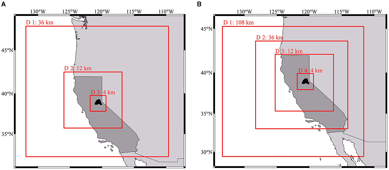
Figure 2. WRF domain configurations for (A) the 3-domain configuration, and (B) and 4-domain configuration. The 3-domain configuration has an outermost domain at a resolution of 36 km, followed by a domain at a resolution of 12 km, and an inner domain centered on ARW at a resolution of 4 km. The 4-domain configuration has an additional outermost domain at 108 km with the same three inner domains at resolutions of 36 km, 12 km, and 4 km.

To run WRF, the main input required is global reanalysis data. For this study, three global reanalysis datasets are provided as inputs to WRF depending on the year being reconstructed. The datasets include the Twentieth Century Global Reanalysis Version 2c (20CRv2c), The European Center for Medium-Range Weather Forecasts twentieth century reanalysis (ERA20C), and the Climate Forecast System Reanalysis (CFSR). 20CRv2c is provided by the Earth System Research Laboratory Physical Sciences Division from NOAA and the University of Colorado Cooperative Institute (Compo et al., 2011). The 20CRv2c reanalysis data are computed by assimilating surface pressure using observed monthly sea surface temperature and sea ice distributions as boundary conditions with an Ensemble Kalman Filter and has a 6-h temporal resolution, 2.0° horizontal resolution and 28 vertical atmospheric layers with data available from 1851 to 2014. ERA20C is provided by the European Center for Medium-Range Weather Forecasts and is computed by assimilating surface pressure and marine winds (Poli et al., 2016). There are 91 vertical atmospheric levels, 4 land surface soil layers, a horizontal resolution of ~125 km and a temporal resolution of either 3- or 6-h depending on the variable. Data are available from 1900 to 2011. Finally, CFSR is provided by the National Centers for Environmental Prediction and data are computed by assimilating satellite radiances using a grid- point Statistical Interpolations Scheme, providing data at a horizontal resolution of ~38 km with 64 vertical atmospheric layers and a 6-h temporal resolution from 1979 to present (Saha et al., 2010). CFSR is considered to be the most comprehensive compared to other reanalysis data due to the use of both ocean and sea ice in its computation and therefore when available, it is the reanalysis data of choice.

In terms of observation data, the main calibration and validation output is basin-averaged precipitation from the Parameter-Elevation Regressions on Independent Slopes Model (PRISM, PRISM Climate Group, 2014). A parameter-elevation regression function at each grid cell is calculated using a precipitation distribution model that interpolates point data, digital elevation maps (DEMs), and spatial data based on the slope orientation and weighted station data. While able to incorporate different spatial scales and orographic precipitation mechanisms, the fundamental assumption within PRISM is that elevation is the deciding factor in the precipitation distribution. The computed data allow the finer scale interactions in mountainous regions to be estimated and considered during the calibration and validation process beyond what point scale observations typically can capture (Ishida and Kavvas, 2017). PRISM data are available at daily, monthly, annual, or event-based periods at a spatial resolution of 4 km. While the main variable used in this study is precipitation, a variety of attributes are available relating to temperature, dew point, vapor pressure.

As discussed previously, because parameterizations of some atmospheric mechanisms are required, WRF needs to be calibrated and validated for the target area. In this case WRF is calibrated for the period from 1997 through 2006 using CFSR input data, and validation is performed from 2007 through 2016, also using CFSR input data and the 3-domain configuration.

2.1.1 WRF calibration

To perform calibration, manual optimization is performed based on different parameterizations of the physics options within WRF for the 3-domain configuration, and outputs are compared to PRISM data. The physics options evaluated include the microphysics, cumulus, surface layer, land surface, and boundary layer parameterizations. The selected options that were ultimately chosen include the SBU-YLin scheme (Lin and Colle, 2011) for the microphysics processes, the New SAS Scheme (Han and Pan, 2011) for the cumulus parameterization, the Eta Similarity Scheme (Janić, 2001) for the surface layer scheme, the RUC Scheme (Smirnova et al., 2016) for the land surface scheme, and the BouLac (Bougeault and Lacarrere, 1989) option for the boundary layer scheme. The calibration period for WRF is from water year 1997 through water year 2006 (October 1, 1996–September 30, 2006). This period encompasses 2 water years that experienced flooding, 1997 and 2006, and eight low to average precipitation water years, 1998 through 2005 (California Nevada River Forecast Center, 1997, 2006). This 10-year period ensures that the WRF configuration is capable of simulating both wet and dry years and is not over calibrated for a certain precipitation regime. CFSR reanalysis data are available for this period, ensuring the highest quality and highest resolution input data are used to calibrate the model.

To evaluate WRF outputs against PRISM data, the Nash-Sutcliffe Efficiency Index (NSE) is used (Nash and Sutcliffe, 1970). NSE has widely been applied as a performance assessment tool for hydrologic models and, in this study, an NSE above 0.5 is considered sufficient in evaluating WRF outputs at both daily and monthly scales. The root mean square error (RMSE) and Pearson correlation coefficient (r) are also considered in the calibration procedure. Final calibration results were successful when comparing both daily and monthly basin-averaged precipitation WRF outputs against PRISM daily and monthly basin-averaged precipitation (Figure 3). At a daily scale, an NSE of 0.82 and an RMSE of 4.3 mm were achieved. At a monthly scale, an NSE of 0.95 and an RMSE of 30.3 mm were achieved. Both results indicate a successful calibration of WRF.

Figure 3

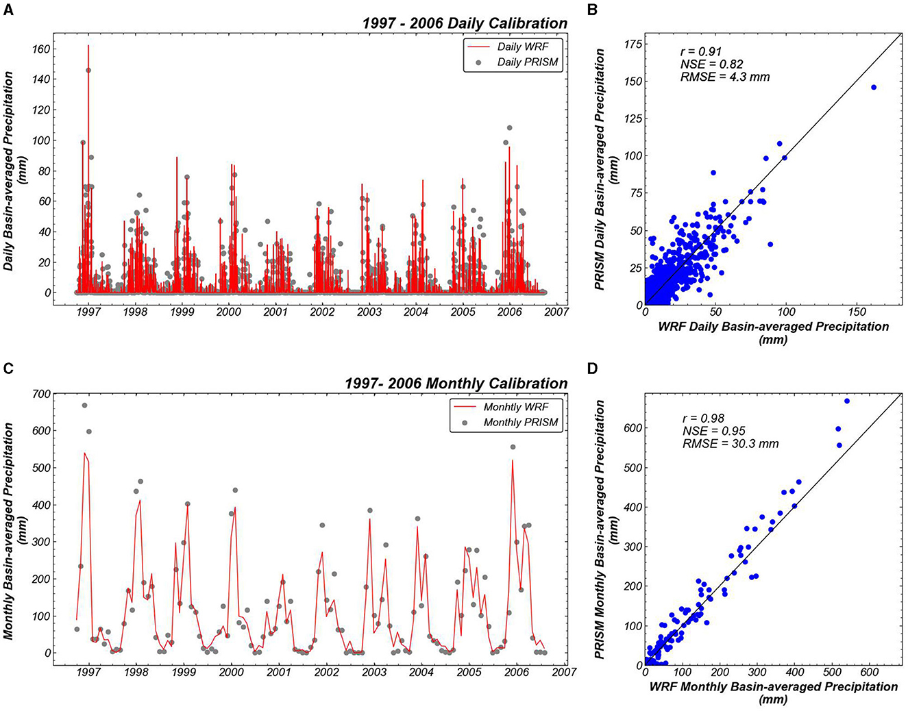
Figure 3. WRF calibration results for the 10-year period from water year 1997 through water year 2006 for (A) daily time series, (B) daily scatter plot, (C) monthly time series, and (D) monthly scatter plot. At the daily scale, a NSE of 0.82 and a RMSE of 4.3 mm was achieved with a correlation coefficient of 0.91. At the monthly scale, a NSE of 0.95, a RMSE of 30.3 mm, and a correlation coefficient of 0.98 was achieved for the cumulative basin-averaged precipitation.

Looking first at the daily scale, a correlation coefficient of 0.91 indicates a strong positive linear relationship between WRF outputs and PRISM data. WRF slightly overestimates the largest daily peak in precipitation in 1997. At a precipitation of around 100 mm, the datasets either match well or PRISM is slightly larger compared to WRF. At lesser daily precipitation values, however, there is a fairly even spread centered around a 1:1 relationship even if the precipitation values do not match perfectly. At the monthly scale, a correlation coefficient of 0.98 is achieved, indicating an excellent match between WRF monthly basin-averaged precipitation and PRISM monthly basin-averaged precipitation. Though, it should be noted that at monthly values greater than about 350 mm, PRISM is tending to overestimate results compared to WRF outputs. At both time scales, the NSE values exceed the 0.5 threshold, the RMSE is sufficiently small, and the high correlation coefficients establish that the WRF configuration is appropriate, and the model is considered calibrated for ARW.

2.1.2 WRF validation

Following the successful calibration of WRF, the model must be validated against additional data with the 3-domain configuration. The validation period is an additional 10-year period from water year 2007 through water year 2016 (October 1, 2006–September 30, 2016). CFSR data are available for this entire period and are thus used as the input atmospheric data. The validation results for both the daily and monthly scales of basin-averaged precipitation are again successful (Figure 4). The daily basin-averaged precipitation against PRISM data resulted in an NSE of 0.85 and an RMSE of 3.7 mm. For the monthly cumulative basin-averaged precipitation, an NSE of 0.95 and an RMSE of 24.6 mm were achieved. With NSE values >0.5, the WRF model is considered sufficiently validated.

Figure 4

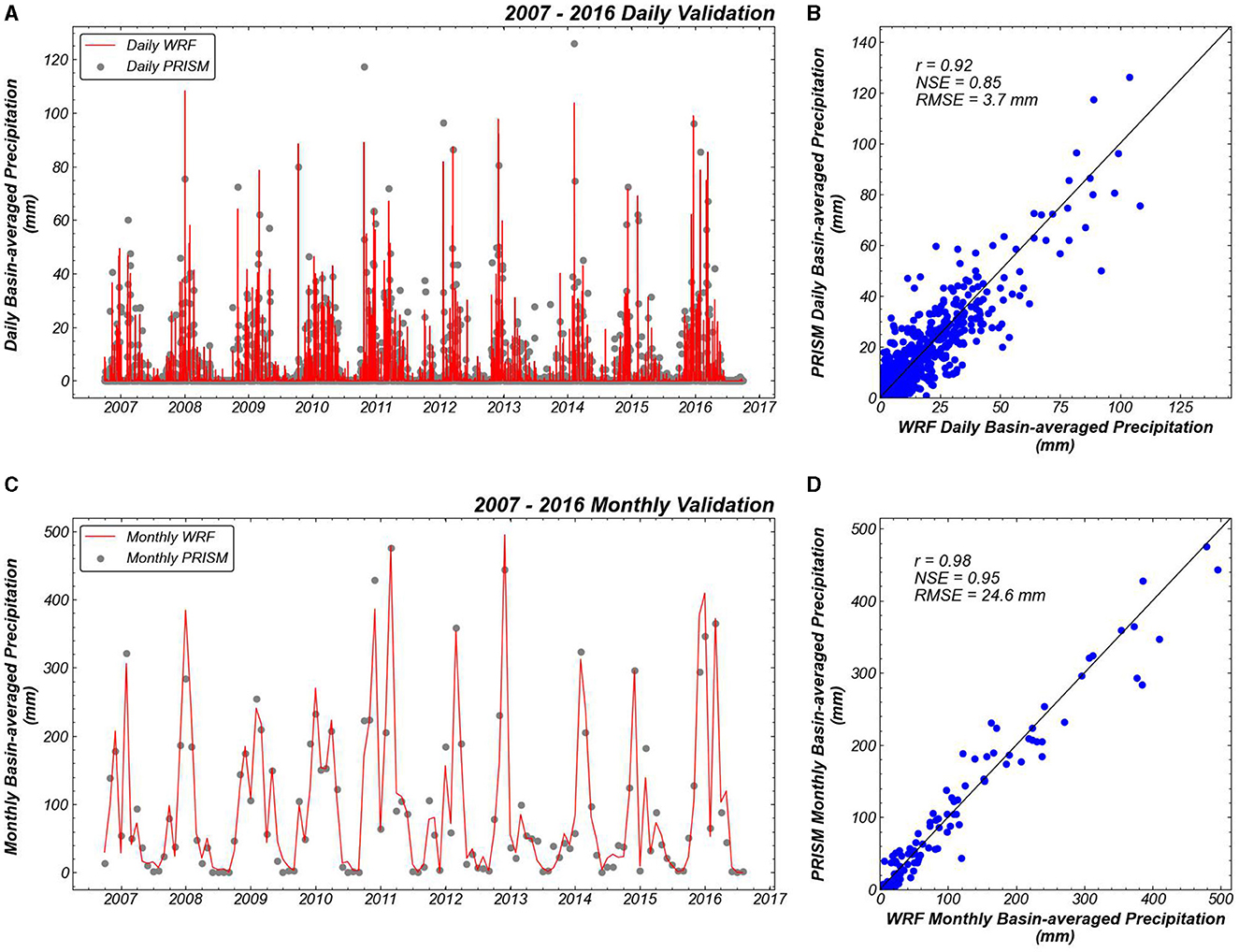
Figure 4. WRF validation results for the 10-year period from water year 2007 through water year 2016 for (A) daily time series, (B) daily scatter plot, (C) monthly time series, and (D) monthly scatter plot. At the daily scale, a NSE of 0.85, a RMSE of 3.7 mm, and a correlation coefficient of 0.92 was achieved. At the monthly scale for the cumulative basin-averaged precipitation, a NSE of 0.95, a RMSE of 24.6 mm, and a correlation coefficient of 0.98 was achieved.

As with the calibration a strong positive relationship is seen for the validation with a daily correlation coefficient of 0.92 and a monthly correlation coefficient of 0.98. While there is similar spread in the daily precipitation under about 70 mm between the calibration and validation results, more variability is seen at higher precipitation values. The most apparent being the underestimation by WRF for the 2011 and 2014 peak daily precipitation in addition to the overestimation by WRF in 2008 and to a lesser extent 2013. At the monthly scale, results are again excellent. Whereas, calibration results underestimated WRF monthly basin-averaged precipitation at values >350 mm, validation results indicate that WRF tends to match or overestimate precipitation compared to PRISM data. Even with these slight differences, WRF is considered sufficiently validated, and outputs can be used as inputs to run the WEHY-HCM system.

2.2 WEHY-HCM SNOW Module

The SNOW Module of WEHY-HCM is necessary as it has been estimated that for ARW snowmelt contributes between 50 and 80% of spring and summer streamflow as the temperatures rise and the precipitation stored in the snowpack is released (Stewart et al., 2004). Fully accounting for the snow regime is thus critical to successfully simulate flow both as it accumulates and later melts. However, the complex interactions between the non-stationary atmospheric forcings and the changing snow structure are difficult to model and computationally intensive as a fine spatial and temporal resolution is required (Welty and Zeng, 2021). As such, the WEHY-HCM SNOW Module is implemented as it can further simulate the land-atmosphere interactions controlling the snow regime as ARW is a snow driven watershed.

The SNOW Module was developed to understand and simulate the non-uniform vertical temperature profile of the snowpack, which is dictated by atmospheric interactions in the top, skin layer of the snowpack (Ohara and Kavvas, 2006). As a physically based, energy budget model, the module uses input atmospheric and land data to estimate the energy exchange between the snowpack and the surrounding environment by numerically solving the conservation of mass and energy equations in the snowpack. At every node in the grid network, the snowpack is divided into three layers. The top, skin layer incorporates the atmospheric forcings. Below that is the active layer, above the evolving freezing depth, where a linear temperature profile is assumed. Finally, the lowest level, below the freezing depth, is isothermal at 0°C and disconnected from any atmospheric interactions. To account for topography and elevation effects at each grid point, DEMs provide land data to compute the solar angle and calculate the incoming solar radiation which is used to solve the energy budget. Across the domain, these point scale processes are vertically integrated over the snowpack depth and numerically upscaled to produce a spatially distributed model which contains both the atmospheric forcings and the solar geometry, accounting for the spatial heterogeneity of snow accumulation and melting processes.

Input data required by the SNOW Module include atmospheric data provided by WRF, DEM data, vegetation and LULC data, and geomorphological data (Figures 1A–C). To incorporate the spatial heterogeneity in the mountainous region of ARW, fine scale DEM data, at a resolution of 30 m, is used, provided by the USGS National Elevation Dataset. Similarly, fine resolution LULC, provided by the California Department of Forestry and Fire Protection, and geomorphological data, provided by the US Department of Agriculture's Web Soil Survey, are also required. Following the delineation of the land characteristics of the watershed, the SNOW Module needs to be calibrated and validated specifically for ARW before reconstruction can be done.

2.2.1 SNOW Module calibration

For calibration of the SNOW Module, outputs are again compared to observation data related to snow conditions, with the focus being on snow water equivalent (SWE). Snow cover observation data are limited and thus for the calibration and validation process, point scale observations are instead used. The California Data Exchange Center (CDEC) publishes a variety of observation data at different time scales. Within ARW, there are six CDEC observation stations that collect daily SWE in the period used for calibration and validation (Figure 1A). Physical characteristics and the start date of daily SWE observations for each of the six stations are noted in Table 1. The expected snow cover over the winter is greatly dependent on the elevation of the station. Three of the stations (ALP, CAP, and LOS) are in the higher-elevation headwaters of ARW where significant and persistent snow cover is expected through the winter months compared to the three mid-elevation stations (BLC, GKS, and RBP) where the snowpack is expected to have a lower magnitude and be more variable over the winter months.

Table 1

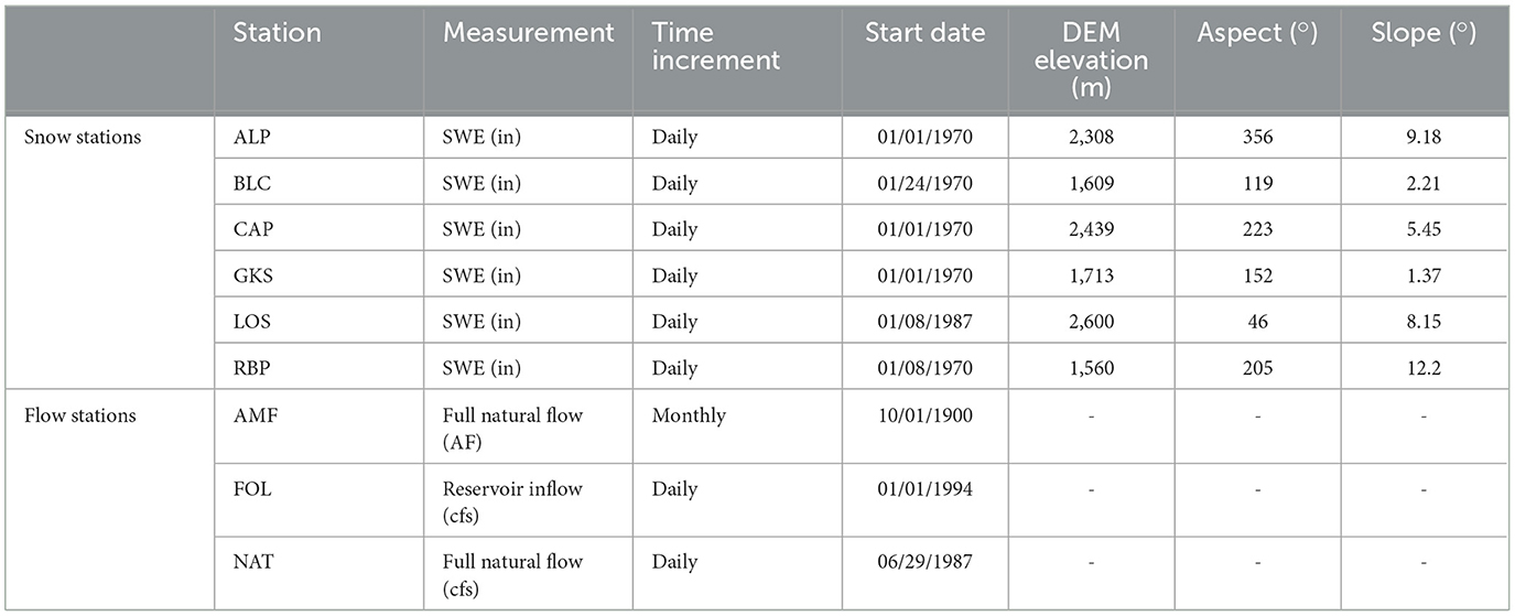
Table 1. CDEC station details for the observation data used to calibrate and validate WEHY-HCM and the SNOW Module.

As a physically based model, parameters need to be calibrated within the SNOW Module. The parameters that are changed are primarily related to albedo. Other parameters are physically based constants, and typically are not changed during the calibration process. Using the calibrated WRF model outputs, the SNOW Module is run, and the point scale outputs are compared to each of the six CDEC observation points. To maintain consistency, the calibration period is again the 10-year period from water year 1997 through water year 2006 (Figure 5). NSE values for SWE calibration are only calculated for the days with available observation data. Because there is no modeling involved in the SWE observation data, there may be significant portions of missing data in the record such as at ALP, which is missing the entirety of the 2005 water year, at BLC, which is missing the entirety of the 2001 and 2002 water years, and at LOS, which is missing most of the 1997, 1998, 1999, and 2002 water years. Despite this, there is still sufficient observation data to perform a successful calibration.

Figure 5

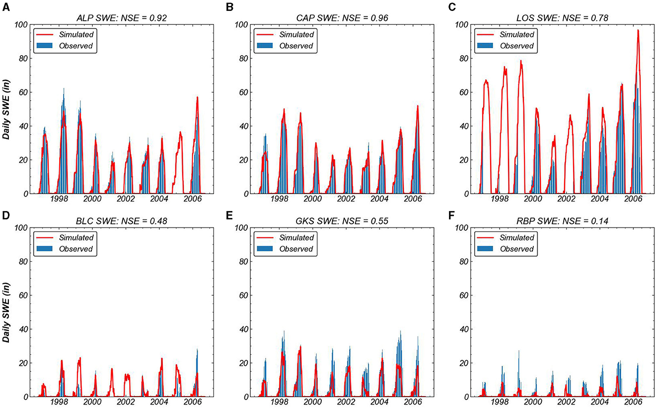
Figure 5. SNOW Module calibration using daily SWE data compared to CDEC observation data at the (A) ALP, (B) CAP, (C) LOS, (D) BLC, (E) GKS, and (F) RBP stations. At the stations in the ARW headwaters, NSE values of 0.92 at ALP, 0.96 at CAP, and 0.78 at LOS are achieved. At the mid-elevation stations NSE values of 0.48 at BLC, 0.55 at GKS, and 0.14 at RBP are achieved. Though all six point-scale daily SWE NSE results do not pass the 0.5 threshold, the module does perform well in the locations where significant and persistent SWE is expected.

First considering the higher elevation stations above 2,000 m, excellent daily NSE values are achieved for the calibration period: 0.92 for ALP, 0.96 for CAP, and 0.78 for LOS. These three stations have both significant accumulation and persistent snow cover over each winter period, as expected. At the mid-elevation stations, between 1,000 and 2,000 m, daily NSE values are more variable, with only one of the three stations passing the 0.5 NSE threshold set for calibration and validation. The resulting NSE values are 0.48 at BLC, 0.55 at GKS, and 0.14 at RBP. At the two stations that did not pass the 0.5 NSE threshold, BLC and RBP, SWE is typically below a peak of 20in and are much more variable over the winter, with sharp peaks and declines in SWE as accumulation and melting processes are dependent on the variable temperature at the station elevation. Given that the point scale daily SWE NSE results exceed the established threshold for the three higher elevation stations, where snow accumulation will persist into spring and contribute to snowmelt driven flow, and significantly lower than the 0.5 NSE threshold at only one station (RBP) the WEHY-HCM SNOW Module is considered successfully calibrated for ARW.

2.2.2 SNOW Module validation

Following a successful calibration, the SNOW Module must also be validated for an independent dataset. As with WRF, the validation period is from water year 2007 through water year 2016 (Figure 6). Similar trends that are seen in the calibration period are again apparent in the validation period. The three stations in the headwaters of ARW perform well, with NSE results >0.8. Additionally, the BLC and GKS stations also pass the 0.5 NSE threshold. While the RBP station does not pass the threshold, with a NSE result of 0.36, results are improved upon compared to the calibration. With all stations, except one, meeting the NSE threshold, the point scale validation of the SNOW Module is considered successful, and outputs can be used as input to the hydrologic portion of WEHY-HCM.

Figure 6

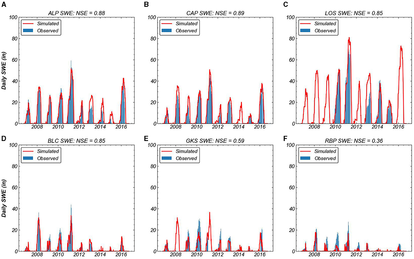
Figure 6. SNOW Module validation using daily SWE data compared to CDEC observation data at six stations (A) ALP, (B) CAP, (C) LOS, (D) BLC, (E) GKS, and (F) RBP for the period from 2007 to 2016. NSE results of 0.88 for ALP, 0.85 for BLC, 0.89 for CAP, 0.59 for GKS, 0.85 for LOS, and 0.36 for RBP are achieved. All stations except the RBP station pass the 0.5 threshold, indicating a successful validation.

2.3 WEHY-HCM

The final model used in this study is WEHY-HCM, which has been applied successfully to numerous mountainous, orographic precipitation driven watersheds in California and internationally (Chen et al., 2004; Trinh et al., 2022). As a physically based hydrology model, WEHY-HCM computes various flow processes at different temporal and spatial scales by numerically solving upscaled versions of the conservation of mass, momentum, and energy equations (Kavvas et al., 2004). Upscaling to the computational grid scale is done by performing an ensemble average of the point scale conservation equations. For the target watershed, the basin is delineated into model computational units (MCUs) with a fundamental assumption that the land parameters are spatially stationary over the individual MCUs. At each MCU, surface and subsurface processes are computed by using unsaturated flow to link the overland flow, subsurface flow, and groundwater flow domains. The upscaled conservation equations are numerically solved, and the unsteady, non-uniform flow discharge from each MCU is then routed through the delineated stream network by the channel flow component of WEHY-HCM to the watershed outlet point.

Physical land characteristics are needed, including topography, geomorphology, and LULC, which are used as physically based parameters in WEHY-HCM to solve the governing equations. By utilizing high resolution land data, the spatial heterogeneity of the target watershed can be accounted for. Additionally, the soil data that are necessary allow the interactions between the land and atmosphere in the boundary layer to be accounted for by coupling the dynamic interactions through vertical fluxes at hillslope scale averages.

The input data required by the hydrologic component of WEHY-HCM are the same as those of the SNOW Module. As with the SNOW Module, surface land data include DEM, geomorphological, soil, and LULC data (Figures 1A–C). The DEM data are used to delineate the basin of interest for an outlet point. For ARW, a total of 54 MCUs and 17 stream reaches are ultimately selected with the outlet point being Folsom Reservoir (Figure 1D). SNOW Module outputs combine the necessary snow variables with the WRF atmospheric data to create a single WEHY-HCM input file. As with the two previous models, the hydrologic component of WEHY-HCM must also be calibrated.

2.3.1 WEHY-HCM calibration

The calibration point for ARW is selected as the delineated watershed outlet point, which is Folsom Reservoir. Flow observation data are also published by CDEC, and three stations are located near Folsom Reservoir, and can be used to compare against WEHY-HCM outputs during both calibration and validation periods, detailed in Table 1. The NAT station measures daily full natural flow (FNF), the FOL station measures daily inflow, and the AMF station measures monthly FNF volumes. While FOL inflows are used for calibration and validation, FNF is preferred as it computes the flow based on the assumption of no upstream water storage infrastructure, as does WEHY-HCM. Within ARW, there are limited upstream storage structures, and thus, inflow and FNF data are similar with variation predominantly related to flow magnitude.

The main parameters used to calibrate the model are related to the soil depth, saturated hydraulic conductivity, summer and winter albedo, and summer and winter roughness. Other parameters related to land data are used but typically do not need to be changed to calibrate the model. Daily and monthly calibration results for the period from the water year 1997 through the water year 2006 are successful (Figure 7). At the daily scale, an NSE of 0.72 and an RMSE of 4,357 cfs were achieved for inflow at the FOL station, and for FNF at the NAT station an NSE of 0.69 and an RMSE of 4,725 cfs were achieved. The correlation coefficient for daily inflow is 0.86 and for daily FNF is 0.84. The results for inflow vs. FNF are better due to the lower magnitude flow of the inflow observations. During the calibration period, flow into Folsom is typically under ~60,000 cfs, and for those values, there is an even spread around a 1:1 relationship between observations and WEHY-HCM outputs. Beyond that, the daily peak flows seen in 1997 and 2006 are again centered around the 1:1 relationship. The largest daily peak observed for the 1997 flood is overestimated by WEHY-HCM, though the overestimated daily precipitation and SWE during the WRF and SNOW Module calibration may have contributed to that result.

Figure 7

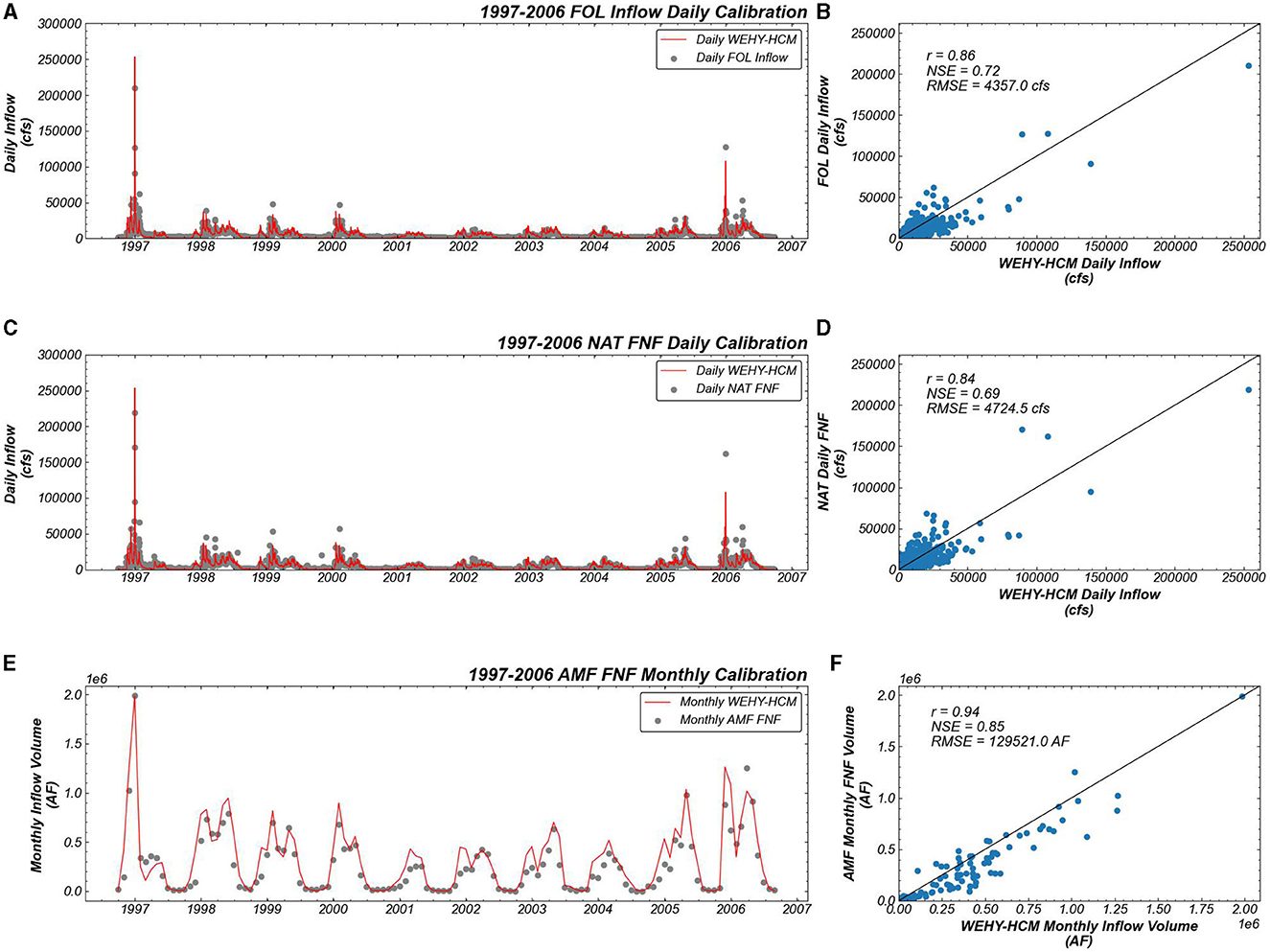
Figure 7. WEHY-HCM calibration for the outlet point at Folsom Reservoir compared to three CDEC observation stations: (A) daily inflow time series and (B) daily inflow scatter plot at the FOL station, (C) daily FNF time series and (D) daily FNF scatter plot at the NAT station, (E) monthly FNF time series and (F) monthly FNF scatter plot at the AMF station. Daily inflow at the FOL station produces a NSE of 0.72, a RMSE of 4,357 cfs, and a correlation coefficient of 0.86. Daily FNF inflow at the NAT station produced a NSE of 0.69, a RMSE of 4,725 cfs, and a correlation coefficient of 0.84. The monthly FNF inflow volume at the AMF station produced a NSE of 0.85, a RMSE of 129,521 AF, and a correlation coefficient of 0.94.

At the monthly scale, FNF volumes at the AMF station achieve an NSE of 0.85, an RMSE of 129,521 AF, and a correlation coefficient of 0.94. At this scale, variations at the daily scale are smoothed out and produce excellent calibration results, particularly for the 1997 peak monthly volume. It should be noted, however, that this WEHY-HCM calibration tends to overestimate the monthly volumes compared to AMF FNF monthly volume, though the model still does well in simulating the observed flow. With all three station comparisons passing the 0.5 NSE threshold, WEHY-HCM is considered calibrated for ARW.

2.3.2 WEHY-HCM validation

The final step before starting reconstruction is to validate WEHY-HCM. To include a higher flow water year, the validation period was extended one year to add the 2017 water year. Thus, the period is 11 years from water year 2007 through water year 2017. Results are again sufficient, with all three station comparisons passing the NSE threshold (Figure 8). NSE values are 0.67 for daily inflow at the FOL station, 0.68 for daily FNF inflow at the NAT station, and 0.78 for FNF inflow volumes at the AMF station. Correlation coefficients are 0.85 for both daily inflow and FNF, and 0.93 for monthly FNF volume. At the daily scale, both results sufficiently surround the 1:1 relationship though it is apparent the results are skewed toward WEHY-HCM overestimating the flow compared to observations. The overestimation by WEHY-HCM is also seen in the monthly volume results, though the 2017 peak months are well-represented. With all three models successfully calibrated and validated, reconstruction can be done for the entire period from 1852 to 2020.

Figure 8

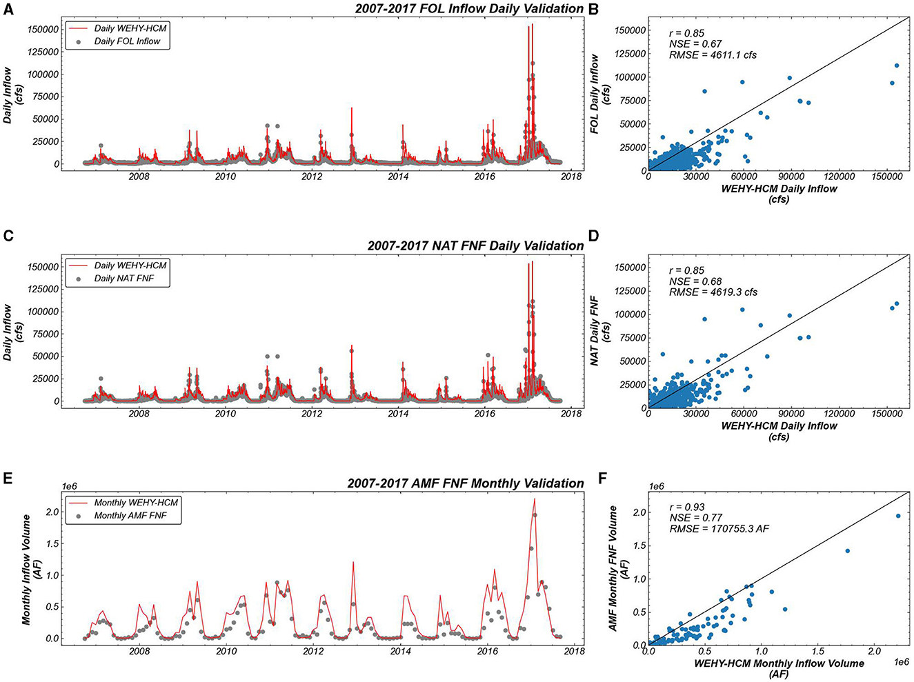
Figure 8. WEHY-HCM validation for the outlet point at Folsom Reservoir compared to three CDEC observation stations: (A) daily inflow time series and (B) daily inflow scatter plot at the FOL station, (C) daily FNF time series and (D) daily FNF scatter plot at the NAT station, (E) monthly FNF time series and (F) monthly FNF scatter plot at the AMF station. Daily inflow at the FOL station produced a NSE of 0.67, a RMSE of 4,611 cfs, and a correlation coefficient of 0.85. Daily FNF inflow at the NAT station produced a NSE of 0.68, a RMSE of 4,619 cfs, and a correlation coefficient of 0.85. The monthly FNF inflow volume at the AMF station produced a NSE of 0.77, a RMSE of 170,755 AF, and a correlation coefficient of 0.93.

3 Reconstruction results

Reconstructing the atmospheric and hydrologic conditions of ARW involves selecting the input reanalysis data and using WRF and WEHY-HCM with the SNOW Module to simulate each water year. Atmospheric data are available starting in water year 1852, and following the validation procedure for WRF, each water year is individually simulated with the available reanalysis data and compared to PRISM observation data, when available. This ensures the individual water years perform well both with the calibrated WRF model and the 3-domain configuration. From 1980 to 2016, CFSR reanalysis data are used as WRF inputs, and all years performed sufficiently with the 3-domain configuration. For 1900 to 1979, both 20CRv2c and ERA20C reanalysis data are available. Each year in this period is simulated twice, to assess both reanalysis datasets. The better of the two simulations compared against PRISM monthly basin-averaged precipitation is selected to be used in the reconstruction time series. If neither of the two reanalysis datasets produce an NSE > 0.5, the WRF 4-domain configuration is then used to rerun the simulations and the better performing results are then selected for that water year. From 1852 to 1899, only 20CRv2c reanalysis data are available. Additionally, no observation data are available, so the reconstruction is limited to the WRF 3-domain configuration. Out of the 169-year reconstruction period, only 3 years needed the 4-domain configuration: 1910, 1914, and 1922. All other years performed sufficiently with the 3-domain configuration.

Following the WRF atmospheric reconstruction, the outputs are run through WEHY-HCM and the SNOW Module to reconstruct the flow conditions. Basin-averaged precipitation and inflows to Folsom Reservoir are the primary outputs of interest. The continuous time series at both the daily and monthly scales are plotted against observation data, where available (Figure 9). Computing NSE values for the entire period, where observations are available, indicate that the models can capture historic atmospheric and hydrologic conditions in ARW. PRISM daily basin-averaged precipitation is available starting in 1981 and compared to WRF outputs, an NSE of 0.71 and a correlation coefficient of 0.86 are achieved. PRISM monthly basin-averaged precipitation is available starting in 1895, and an NSE of 0.87 and a correlation coefficient of 0.94 are achieved. For the flow reconstruction, daily FNF data at the NAT station are available beginning in 1987, and an NSE of 0.56 and correlation coefficient of 0.83 are computed against WEHY-HCM outputs. At the monthly scale, FNF inflow volume at the AMF station is available starting in 1900 and an NSE of 0.60 and a correlation coefficient of 0.84 are computed.

Figure 9

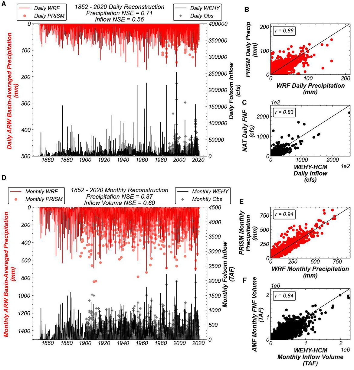
Figure 9. Reconstruction results for ARW basin-averaged precipitation (red) and Folsom Reservoir inflows (black) for daily (A) time series, (B) precipitation scatter plot, and (C) inflow scatter plot and monthly (D) time series, (E) precipitation scatter plot, and (F) FNF volume scatter plot. PRISM observations and CDEC FNF observations are also plotted. NSE results where observation data available are computed. Daily basin-averaged precipitation produced an NSE of 0.71 and correlation coefficient of 0.86, daily FNF inflow produced an NSE of 0.56 and a correlation coefficient of 0.83, monthly basin-averaged precipitation produced an NSE of 0.87 and a correlation coefficient of 0.94, and monthly FNF inflow volume produced an NSE of 0.60 and a correlation coefficient of 0.84.

Considering the precipitation results, at the daily scale there is additional spread in the lower values, below ~100 mm, compared to the calibration and validation periods. At these lower values, WRF both under and overestimates precipitation results. However, at the higher daily precipitation values, above 100 mm, WRF tends to overestimate the basin-averaged precipitation. At the monthly scale, these daily variations are smoothed, and the correlation coefficient results improved, as expected. It is also apparent that WRF tends to underestimate some peak monthly sums, especially further back around 1900. Despite this, the daily and monthly precipitation results are acceptable, and the 169-year period is fully reconstructed to form a continuous, daily basin-averaged precipitation dataset for ARW.

Similarly, for both daily inflow and monthly inflow volumes, spread around the lower ranges of the linear relationship between simulation results and observation values exist. Results follow the tendencies seen in the calibration and validation periods. For daily FNF inflow, there is an even spread between WEHY-HCM both underestimating and overestimating flow compared to the FNF observed at the NAT station. Additionally, at the monthly scale for inflow volumes, there is an apparent bias for WEHY-HCM to overestimate results, particularly between ~1,000 and 2,000 TAF. Greater than 2,000 TAF, however, WEHY-HCM does well to capture the monthly peak inflow volumes. It is also seen in the monthly time series that early in the reconstruction period where observations are available, WEHY-HCM underestimates peaks while seeming to improve, or overestimate, closer to the present. With NSE and correlation coefficient results being satisfactory, the WEHY-HCM system has reconstructed the snow and flow conditions for the full reconstruction period.

Thus, the daily reconstruction of the historical atmospheric, snow, and hydrologic conditions from 1852 through 2020 using WRF and WEHY-HCM with the additional SNOW Module are complete. This continuous, detailed dataset with a long period of record will allow further analysis on the hydroclimate conditions in ARW before the current observation network was established. Analysis can be done across various timeframes, to look at long term trends, or for specific events. By modeling the entire hydroclimate system, a better understanding of the interactions between the land surface and atmosphere that lead to historic extreme events can be studied. In addition to the time series dataset that has been created, the spatial data of all variables is also available. This is particularly useful when ROS events occur, and the spatial distribution of liquid precipitation and snow cover is vital to assessing the resulting streamflow. Before using this dataset in future studies, the results of specific historical events should be further considered.

4 Discussion

While the full period reconstruction of the atmospheric and hydrologic conditions in ARW using three physically based models is successful, it is necessary to consider model results under specific flow conditions. By analyzing basin averaged precipitation and temperature, two SWE stations, and the inflow to Folsom reservoir, the interactions within the hydroclimate system can be considered together to examine how the watershed responds to different conditions. The role of temperature in producing ROS flood events can also be explicitly considered to provide more insight into the processes leading to these types of events.

In the reconstruction period, there have been numerous periods of extreme flooding and prolonged droughts. Since the three models have been calibrated and validated, more distant past years with extremes can be further analyzed. However, for the purpose of this study, further analysis of extreme conditions is limited to those years with observation data, to directly compare modeled results to observed conditions. The goal is to understand how interactions between the atmosphere and land surface contribute to producing both wet and dry extremes.

4.1 Performance under flood conditions

To assess the system performance under flood conditions, three individual water years are considered: 1997, 2006, and 2017. The three years selected contain the largest daily peak flows where observation data are available. While previous years also experienced significant flooding events, such as in 1986, daily flow data are not available prior to 1987.

4.1.1 Water year 1997: the transition between wet and dry conditions in a water year

The flood event in early January of 1997 was significant for ARW, as it was considered the flood of record at that time (California Nevada River Forecast Center, 1997). A wet December contributed substantial snowpack and soil moisture across the watershed, and when a series of atmospheric rivers made landfall, the flood control system was tested as mid-elevation snowpack melted and contributed to the rising flows. An additional aspect of the 1997 water year that must be considered is the fact that following the January flood, the rest of the year was relatively dry, with very little precipitation falling after January. The abrupt transition between wet and dry conditions is especially important for managing the water supply, as operators must decide how much to release ahead of a potential flood while not excessively depleting the supply. With this newly created dataset, potential adaption options can be explored, to test the system under various flow alternatives.

The WRF and WEHY-HCM reconstruction of the water year proves successful. Through WRF, the daily basin-averaged precipitation and basin-averaged temperature are simulated and can be compared to PRISM observations. In terms of precipitation, an NSE of 0.84 and an RMSE of 6 mm are computed (Figure 10A). WRF outputs slightly overestimate the daily peak on January 1, 1997, but for other major peaks WRF outputs either match PRISM well or slightly underestimate the winter precipitation. Looking at accumulated monthly sums, a NSE of 0.96 is achieved, though PRISM estimates December and January sums to be greater than those simulated by WRF. The overview of the water year is also well-simulated, with a wet December and January transitioning to very dry conditions in February and the remainder of the year. In terms of temperature, a daily NSE of 0.88 and an RMSE of 2.3°C are computed (Figure 10B). WRF outputs follow the daily trends in temperature that are computed from PRISM. On warmer days, WRF may underestimate the temperature compared to PRISM and on colder days, such as in mid-January, WRF may simulate cooler temperatures. However, for the most part, differences are slight, and the model can capture the trends in both precipitation and temperature. At the monthly average scale, temperatures are similar with a resulting NSE of 0.98, though WRF underestimates the basin-average temperature more significantly in February, March and to an extent May.

Figure 10

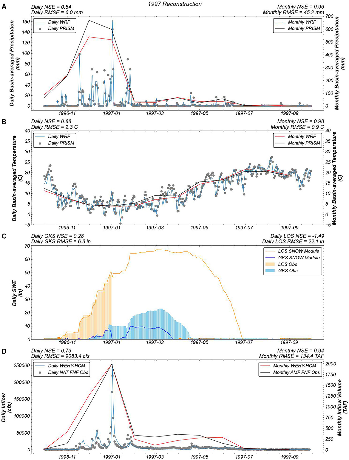
Figure 10. Reconstruction of the 1997 water year against observations for (A) the daily and monthly accumulation of basin-averaged precipitation, (B) the daily and monthly averaged basin-averaged temperature, (C) daily SWE at the LOS and GKS observation stations, and (D) the daily inflow and monthly accumulated volume.

To investigate the SNOW Module performance, two station locations are further assessed (Figure 10C). For the higher elevation areas, the LOS station is considered, as it has average, yet persistent snowpack over the winter. For the mid-elevation areas, the GKS station is considered. Though snowpack will be smaller, the temperature dependent variation of accumulation and melting can be included in the analysis. At the LOS station, observations are inconsistent after January 1, though prior to that, simulation results are excellent. Following the peak January precipitation, the GKS station maintained and later grew the snowpack through the spring until May. However, the SNOW Module simulated near complete melting in early January before the snowpack reaccumulated with the later January storm. While the SNOW Module does underestimate SWE at the GKS station, the overall trend is well-modeled for point scale comparisons. Additionally, though the melting expected with a ROS event is not explicit within the observation data at these two stations, it is noted that snowpack melting did occur during this flood and contributed to the rise in streamflow, as modeled by the SNOW Module (California Nevada River Forecast Center, 1997).

The resulting daily inflow is well-simulated by WEH-HCM compared to the daily NAT FNF observations, with an NSE of 0.73 (Figure 10D). The initial peak flow in November is modeled to occur slightly later but the following peaks in December are modeled nearly perfectly both in terms of time and scale. The extreme flood in early January 1997 is again well-simulated, though WEHY-HCM overestimates the daily peak. The successive peak in late January is underestimated though that may be due to an underestimation in the daily precipitation and a cooler basin-averaged temperature which would not contribute flow from the snowpack melting. Monthly accumulated simulation inflow volumes also closely match observed FNF at the AMF station, with an NSE of 0.94. Though November and December are overestimated by WEHY-HCM, the January accumulation is a nearly perfect match. Through the spring months, WEHY-HCM then underestimates the accumulated volume, with differences in snowmelt likely playing a role in the underestimation. This water year is included in the calibration period for all three models, and thus it is expected that results should surpass the NSE thresholds established.

4.1.2 Water year 2006: the spatial distribution of snow processes

Following the 1997 record flood, 2006 was the next year that saw significant flows (California Nevada River Forecast Center, 2006). Early dry antecedent conditions were alleviated by the wet November, allowing the watershed to saturate with little increase to Folsom inflows. The prolonged storm period in December, combined with the warm temperatures, led to precipitation falling primarily as liquid with snow limited to the highest peaks in the watershed above the snow line around 2,600 m. The peak rainfall in late December into early January, ultimately resulted in the largest daily inflow as many Northern Sierra Nevada reservoirs saw their rivers rise above the flood stages. However, early reservoir releases ahead of the major storm allowed the high flows to pass without any major incidents.

Reconstructing the water year again proved successful for WRF and the WEHY-HCM system. Daily basin averaged NSE values of 0.88 for precipitation and 0.89 for temperature are achieved (Figures 11A, B). The daily precipitation peaks in December and January are underestimated by WRF whereas the daily precipitation peaks in November and March are overestimated. The high daily variability of this water year is smoothed when considering the accumulated monthly sums. Excellent results are achieved, with an NSE of 0.97, and WRF outputs closely match those estimated by PRISM. The largest differences occur in December and April, where WRF underestimates the accumulated basin-average precipitation. In terms of temperature, WRF again tends to underestimate the warmer days, however, cooler days are well-simulated. At the monthly averages, across the entire year, WRF underestimates the basin-averaged temperature, which may play a role in the SNOW Module simulation results, however, an NSE of 0.97 is still achieved.

Figure 11

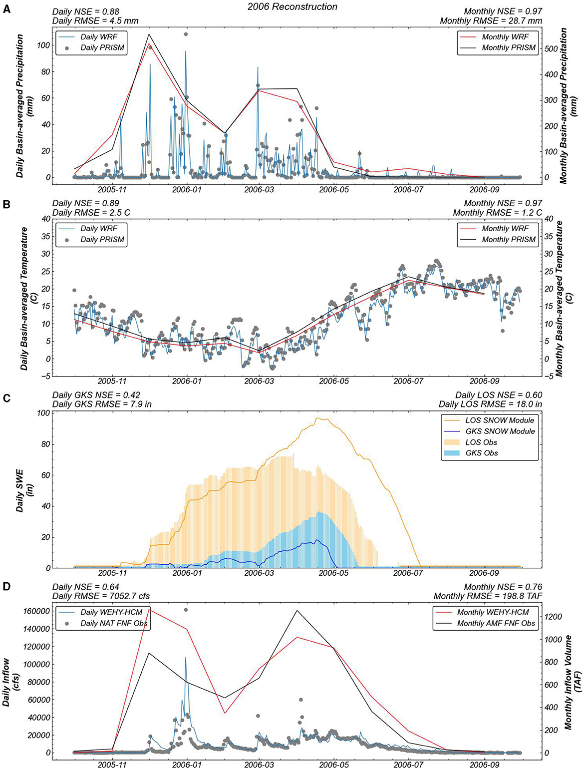
Figure 11. Reconstruction of the 2006 water year against observations for (A) the daily and monthly accumulation of basin-averaged precipitation, (B) the daily and monthly averaged basin-averaged temperature, (C) daily SWE at the LOS and GKS observation stations, and (D) the daily inflow and monthly accumulated volume.

The performance of point scale SWE simulations is mixed (Figure 11C). The GKS station does not pass the 0.5 NSE threshold at 0.43 but the LOS station does at 0.60. At the mid-elevation station GKS, SWE accumulation is minimal through the winter until after the major storm period in early January. Overall, the SNOW Module does underestimate SWE compared to the observations which may be due to the underestimation of basin-averaged precipitation in the storm immediately following the early January flood and the daily peaks in April. At the higher elevation station LOS, SWE simulations follow a similar pattern, initially underestimating SWE compared to the observations. Beginning in March, however, the SNOW Module overestimates SWE as the spring precipitation and cooler temperatures allow snow accumulation to occur.

The simulated daily inflow to Folsom reservoir is again successful with an NSE of 0.64, though the model underestimates, in some instances significantly, the peak flows in January, March, and April (Figure 11D). The initial peak in early December is well-modeled, though the major flood peak in early January is significantly underestimated. Following the major flood, the later, smaller increases in flow in February through the spring, are well-simulated as the small daily variations in flow are captured. Despite the underestimation in daily peaks by WEHY-HCM, the monthly accumulated inflow volumes do not necessarily follow the same pattern. In December and January, where the major daily peak is underestimated by WEHY-HCM, the model simulates larger accumulated volumes. Alternatively, into the spring, where the daily peaks are again for the most part underestimated, WEHY-HCM simulates slightly larger volumes in March but underestimates the sums in April. The role of snow processes is again likely to contribute to the major differences. In the winter months, precipitation is well-simulated, but the higher elevation snow is underestimated, suggesting that despite the cooler temperatures compared to PRISM, more precipitation is contributing to streamflow than is accumulated. One explanation may be the distribution of precipitation that is simulated by WRF. While the basin averaged precipitation may be well-estimated, if WRF simulates additional low elevation liquid precipitation, excessive precipitation will contribute to streamflow as opposed to the snowpack. Into the spring, and in April, specifically, the SNOW Module simulates high elevation snow accumulation whereas observations at the LOS station suggest snowmelt is occurring. The underestimated April precipitation is then further reduced from the resulting streamflow as the snowpack accumulated instead of melting. However, an NSE of 0.76 is achieved for the water year. Overall, the three physically based models do well to model the atmospheric and hydrologic conditions across the watershed and the importance of the snow processes across the watershed are highlighted.

4.1.3 Water year 2017: the difficulty of significant daily variability

The final flood year in consideration is 2017. Particularly for northern California, this wet year was vital in terms of alleviating the long-term drought of the previous 5 years as a record amount of precipitation from October to February was observed (California Nevada River Forecast Center, 2017). The unusually wet October through December provided wet antecedent conditions for the historical precipitation of January and February. Record snow levels were also seen across the Sierra Nevada range and ultimately, the major reservoirs were able to be filled, reducing the threat of water shortages from the preceding drought period.

While the WRF simulation does not pass the NSE threshold of 0.5 at the daily scale, it does capture the high variability of basin-averaged precipitation throughout the water year (Figure 12A). For daily peaks below 100 mm, WRF simulates the observed precipitation within the range of the RMSE result. For the two largest peaks in January and late February, WRF overestimates the daily precipitation. However, this high variability is again smoothed at the accumulated monthly scale, with a resulting NSE of 0.99. Even though the daily WRF outputs do not simulate the exact magnitude of peak precipitation, over the month those differences are reduced. WRF captures the temperature time series well, with a daily NSE of 0.86 and a monthly NSE of 0.96 (Figure 12B). In the winter periods, some days are simulated to be warmer than observations and into the summer WRF generally overestimates the daily temperature. As opposed to the 2006 water year, in 2017, WRF overestimates the average monthly temperature. Particularly in April through the summer, the warmer temperatures likely play an important role in the snow simulation results.

Figure 12

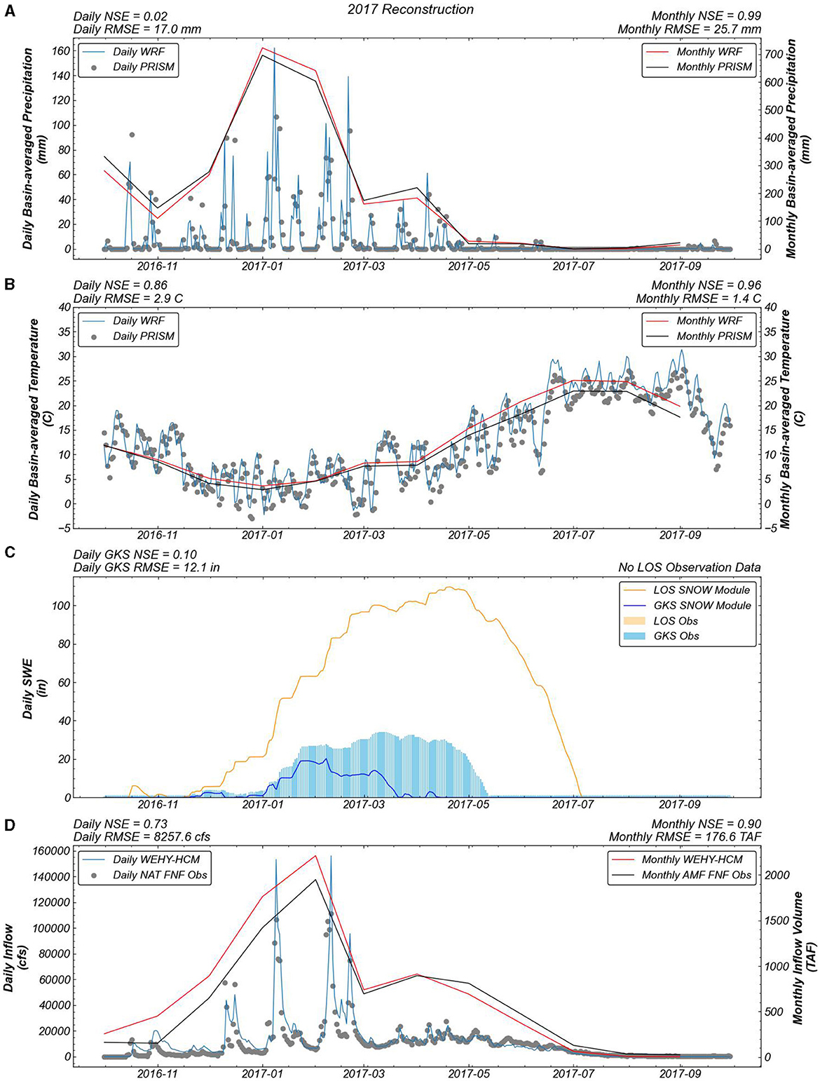
Figure 12. Reconstruction of the 2017 water year against observations for (A) the daily and monthly accumulation of basin-averaged precipitation, (B) the daily and monthly averaged basin-averaged temperature, (C) daily SWE at the LOS and GKS observation stations, and (D) the daily inflow and monthly accumulated volume.

Unfortunately, SWE observations are not available for the 2017 water year at the LOS station, so high elevation snow cover cannot be assessed (Figure 12C). For the GKS station, observations are available, though the SNOW Module underestimates SWE for the entire year. Through early January the module follows the observations closely. However, following the early January storm, the module simulates lower SWE levels and into the spring faster melting compared to the observations.

The combination of differences in both precipitation and snow cover may contribute to the differences seen between the simulated inflow and the AMF FNF observations (Figure 12D). The overestimation of the flow resulting from the January storm is likely due to the overestimation of the precipitation. Additionally, the overestimation of the daily peak flow in early February is likely due to a combination of larger precipitation and greater mid-elevation snowmelt than is observed. The second February peak, while closer to the observed value, is also overestimated, likely due to WRF again overestimating the daily basin-averaged precipitation. Despite the underperformance of WRF in terms of daily basin-averaged precipitation and the SNOW Module in terms of mid-elevation snow processes, the resulting flow from WEHY-HCM is still satisfactory with an NSE of 0.73. For the monthly accumulated inflow volumes, the daily overestimations are carried over as the fall into winter months also exhibit a general overestimation compared to the AMF FNF observations. However, a sufficient NSE of 0.90 is achieved. This water year demonstrates that even if daily simulation results do not meet the established threshold, by assessing the cumulative monthly results, much of the variability can be smoothed to produce sufficient results.

4.2 Performance under drought conditions

In addition to assessing water years that experienced extreme flooding, it is also necessary to assess how the models perform in terms of long-term droughts. With the limitations of observation data, two multi-year periods of droughts in ARW are considered. The first period is from 1987 through 1992 and the second is from 2012 through 2016.

4.2.1 Water years 1987–1992: modeling the dampened water supply

This 4-year period of drought across California followed the record flood for its time in 1986. Precipitation across the regions was three quarters of the recorded average while stream flow was only about one-half of the recorded average (Nash, 1993). As with all droughts, warmer temperatures combined with reduced and warmer reservoir releases severely impacted the endangered salmonoids spawning downstream. Additionally, the diminished streamflow across the region threatened native and endangered riparian and aquatic species. This drought emphasized the need to concurrently manage water resources and natural systems for future droughts. It also highlighted the need to increase monitoring for environmental conditions and resources to be able to quantify the impact of future droughts.

In terms of simulating this 6-year period, WRF performed well for precipitation, with a daily NSE of 0.72, and temperature, with a daily NSE of 0.88 (Figures 13A, B). The reduced precipitation is clearly visible with observations consistently below daily peaks of 80 mm of basin-averaged precipitation. Simulation results are in line with the lessened daily peaks, except for December of 1992, where WRF overestimates the basin-averaged precipitation. At the monthly scale, the accumulated precipitation is also well-modeled with an NSE of 0.90. The winter sums are for the most part well-simulated, though WRF exhibits larger spring sums than is seen in the PRISM estimations of basin-averaged precipitation. The monthly average temperature is also well-simulated, though WRF simulations are slightly smaller compared to PRISM for most of the 6-year period.

Figure 13

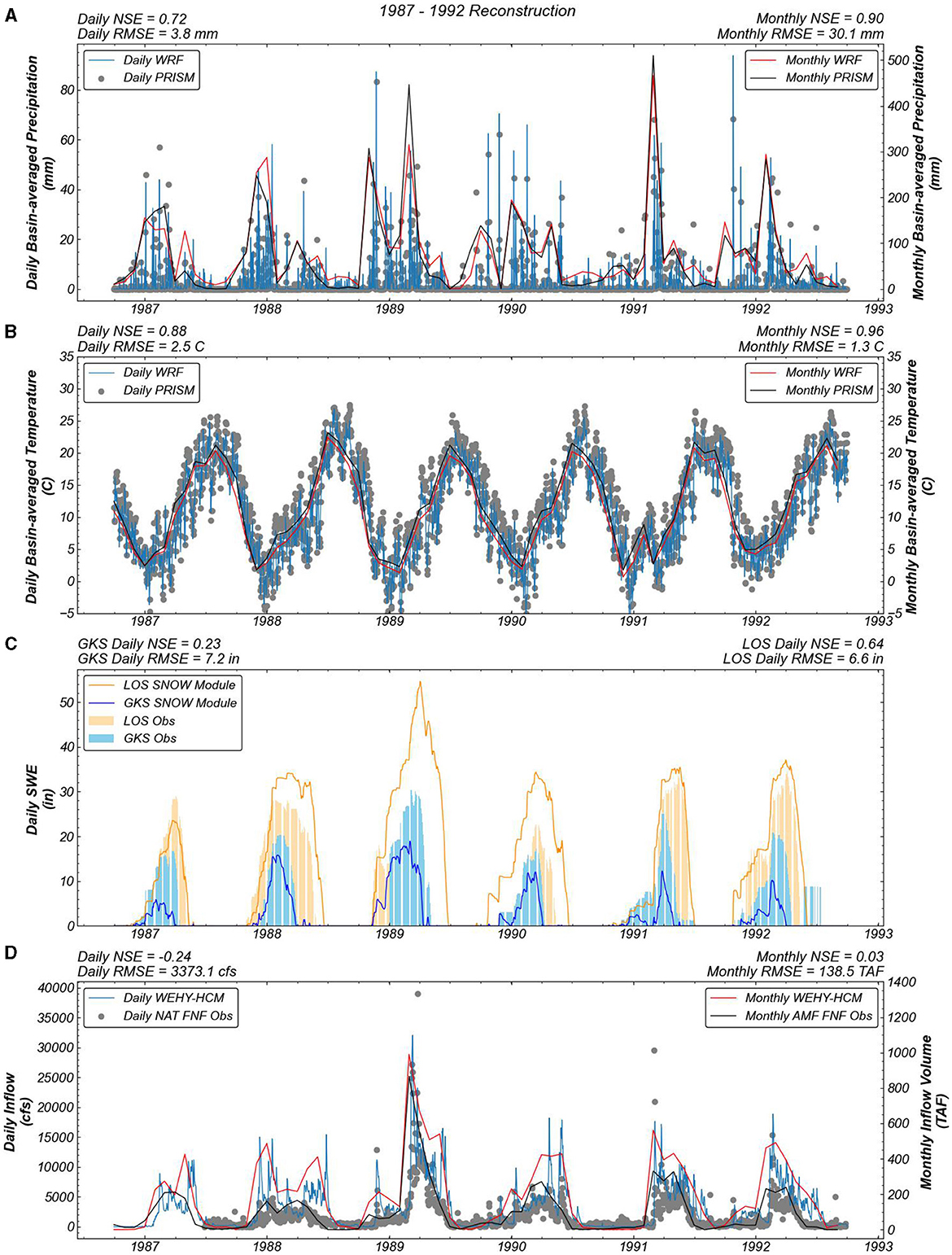
Figure 13. Reconstruction of the drought period from 1987 to 1992 against observations for (A) the daily and monthly accumulation of basin-averaged precipitation, (B) the daily and monthly averaged basin-averaged temperature, (C) daily SWE at the LOS and GKS observation stations, and (D) the daily inflow and monthly accumulated volume.

Snow accumulation is also diminished, particularly in the upper elevations (Figure 13C). At the LOS station, SWE is only modeled to accumulate above 50 in in 1989, which is significantly less than during flood years which saw at least 70 in of SWE in the winter. Though observation data are missing for most years, data that are available are not ever above 40 in. The SNOW Module does well for the LOS station, with an NSE of 0.64. At the GKS station, however, the module underestimates snow for all years, though the timing of accumulation and melting processes is simulated well for the most part.

The under simulated mid-elevation snowpack at the GKS station likely plays a role in the resulting flow not meeting the NSE threshold at either the daily or monthly scales (Figure 13D). The daily inflow peaks in 1989 and 1991 are underestimated, though the monthly accumulated volumes are overestimated by WEHY-HCM. Additionally, numerous larger and more varied daily peaks are simulated which are not seen in the observations. These additional daily peaks contribute to the larger volume that is also simulated by WEHY-HCM across the entire drought period. This may be due to a combination of overestimation of precipitation falling as liquid, which does not contribute to the snowpack and leads to increased runoff than is observed, especially if an ROS event occurs. However, the flows are so dampened, for the most part below 30,000 cfs except in 1989 which peaks near 40,000 cfs, they are comparable to spring inflow during flood years. While the NSE does not satisfy the threshold, the RMSE is computed to be 3,373 cfs, which is less than all 3 flood years considered. The RMSE for the monthly accumulated volume is also comparable to that of the flood years. The dampened daily flow and the accumulated monthly flow volume make differences more obvious for smaller magnitudes of flow and highlight that modeling the entire watershed is difficult when so little water is available.

4.2.2 Water years 2012–2016: modeling the diminished snowpack

Finally, the more recent drought across California from 2012 through 2016 is considered. While shorter drought periods were experienced in the early 2000's, this was the longest drought since the 1987–1992 drought (Lund et al., 2018). Numerous records were set in terms of dryness and reduced snow cover and severe consequences were seen. At a society level, emergency proclamations across the state were issued. The reduced releases and inability to meet demand resulted in increased groundwater pumping to maintain the agricultural system in the San Joaquin Valley. As expected, impacts to the natural environment were seen throughout the system. Central Valley subsidence was revealed by satellite imagery, tree mortality increased, wildfires damages increased, the occurrence of harmful algal blooms increased, and endangered salmonoids were further threatened by the reduction in cold water habitats. However, this drought was not directly related to an extreme lack of precipitation. The precipitation rates were similar to that of previous droughts but the warmer temperatures across the region severely reduced the snowpack and the resulting spring flows.

Again, the daily basin-averaged precipitation and temperature were well-simulated by WRF compared to PRISM observations, with NSE values of 0.82 and 0.87, respectively (Figures 14A, B). Daily precipitation peaks are similar between the two datasets expect in 2014, where WRF underestimates the peak by about 20 mm. At the monthly scale, the accumulated precipitation is also well-simulated with an NSE of 0.95. The winter peaks in precipitation are extremely well-matched, except in 2016 where WRF overestimates the December and January sums. Average temperature is also well-simulated with an NSE of 0.96. While following the trends seen in PRISM, WRF does tend to underestimate the basin-averaged temperature, with the largest differences seen in 2012 and the winter months of the following years.

Figure 14

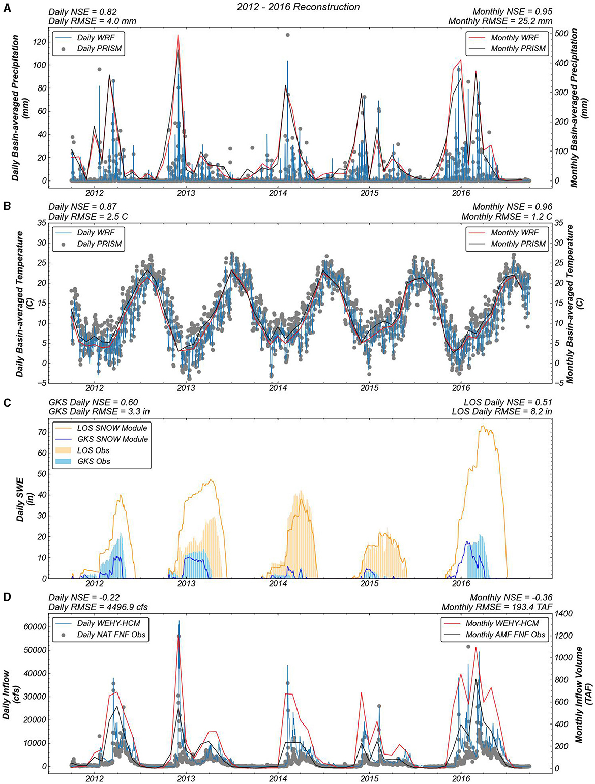
Figure 14. Reconstruction of the drought period from 2012 to 2016 against observations for (A) the daily and monthly accumulation of basin-averaged precipitation, (B) the daily and monthly averaged basin-averaged temperature, (C) daily SWE at the LOS and GKS observation stations, and (D) the daily inflow and monthly accumulated volume.

The impact of the drought on snow processes is clearly seen in the decreased SWE across the 5-year period and the SNOW Module was able to capture this with NSE values of 0.60 at the GKS station and 0.50 at the LOS station (Figure 14C). The reduction in SWE at the GKS station is particularly staggering. All years did not accumulate more than 20 in, and in 2014 and 2015 SWE did not accumulate above 10 in. At LOS, observations are missing for 2012 and 2016 and SWE is overestimated in 2013, but the module does particularly well in 2014 and 2015.

As with the 1987–1992 drought, WEHY-HCM does not pass the NSE threshold for the 2012–2017 drought at both the daily and monthly scales (Figure 14D). However, in this instance, WEHY-HCM better simulates the daily peak flows, likely because the annual peaks are for the most part, except for in 2015, above 30,000 cfs. The similar precipitation to the previous drought in conjunction with the decreased snowpack combine to result in larger daily peak flows. However, for the monthly accumulated inflow volume, WEHY-HCM again overestimates compared to the AMF FNF observations, further highlighting the difficulty in simulating all potential conditions and processes at a watershed scale.

4.3 Overall model performance and limitations

By closely considering the model results for individual water years, general observations can be made about potential model biases. WRF results at a daily and accumulated monthly scale do not follow a specific trend in over or underestimating basin-average precipitation peaks and greatly depend on the year, or years, being simulated. For the SNOW Module, the results at GKS are consistently underestimated compared to observations for all years considered. The results at LOS are more inconsistent, with some years over simulating SWE and some years under simulating SWE. However, this station has a significant number of days without observations, so it is more difficult to draw conclusions. Point scale comparisons are much more difficult to model as opposed to basin-averages due to the complex interactions and non-linearity of the system, in addition to the high resolution necessary, and that is seen in the SWE comparisons. At the GKS station specifically, any differences between the simulated precipitation and temperature against the observations is exacerbated by the smaller SWE magnitudes and the high daily variability in coverage. The impact of precipitation falling as liquid, and potentially melting the snowpack through ROS events, or accumulating and adding to the snowpack significantly impact the downstream flow results. Inflow peaks at the daily scale do not necessarily follow a specific trend in over or underestimating values compared to FNF observations. However, for the monthly accumulated volumes, particularly for drought periods, WEHY-HCM overestimates values when compared against the AMF FNF observations even if the peaks in daily inflow are underestimated.

These results highlight some important points that must be kept in mind when using physically based models. Firstly, the calibration and validation periods that are selected can be vital for later results. If any model is over calibrated for a particular condition, any variation from that will likely result in worsened results. The 10-year calibration and validation periods used in this study are comprised of both high precipitation, high flow and low precipitation, low flow water years. By using a period that contains both extremes, the current model setups can simulate atmospheric and hydrologic conditions for future flow conditions.

Due to the limited daily flow observation data, direct comparisons are limited to more recent water years. Thus, it is difficult to analyze how the model setup performs in the further past when observations may not be available. Furthermore, any observation data or global reanalysis data that is available for an earlier period, such as the early 1900's and prior, is likely to contain larger uncertainties compared to more recent periods. However, absent more comprehensive observation data, this reanalysis data is a good option to fully understand the hydroclimate of the past. Additionally, any change to the physical characteristics of the watershed is not directly considered as a modern DEM and a single WEHY-HCM set up is used for the entire reconstruction. ARW, as with many Sierra Nevada watersheds, has been altered tremendously with the heavy mining and damming in the region continuing through the early 1900's. Additionally, Folsom reservoir was operational starting in 1956, and thus any previous floods than may have been disastrous for Sacramento would likely not have the same impact today with the added flood protection that the reservoir provides. However, by setting up WEHY-HCM to assess inflows to Folsom, comparisons can be made against observations that are available prior to the construction of the reservoir. And because the model parameters are physically based, any changes to the land characteristics due to climate change can be accounted for as impacts become more apparent and new land data become available.

Finally, the impact that air temperature and snow processes have on the resulting flow conditions is evident and must be fully considered when doing any watershed modeling. Because snow processes are highly location specific, with the temperature, solar angle and aspect of the land controlling the accumulating and melting mechanisms, a high-resolution watershed model that directly accounts for snow, is vital. Slight differences between modeled temperature and the actual conditions across the watershed ultimately control how any precipitation falls within the watershed, affecting the resulting magnitude and timing of flow that is simulated. By utilizing WEHY-HCM with the additional SNOW Module, these complex interactions could be further considered at a higher resolution beyond those available in WRF outputs directly.

4.4 Study implications

By constructing a daily time series with spatial distributions of the atmospheric, snow, and flow conditions in ARW from 1852 through 2020, in the future analysis can be done beyond that of the three flood years and two drought periods presented here. Because the system has been calibrated and validated individually for precipitation, snow, and inflow, outputs for conditions across the hydroclimate system are reliable, which is especially beneficial when limited observation data are available. The spatial distribution of all variables across the entire watershed is also produced by this methodology and can provide further insight into the precipitation distribution, snow cover, and upstream reach flows. The daily reconstruction of the spatial distribution of precipitation can be used to identify regions in the watershed that may be most susceptible to changes in the existing geomorphology and river network while the stream reach timeseries across the watershed can be used to identify areas where environmental monitoring may be vital to capture real-time changes within the watershed (Tucker and Slingerland, 1997; Abed-Elmdoust et al., 2016; Sarker et al., 2019; Singhal et al., 2024). Periods of droughts can also be further analyzed to assess which areas in the watershed experience the driest conditions, providing insights that can be used to reduce wildfire fuel loads in vulnerable areas and assess where flora and fauna will be the most stressed under low flow conditions (Dettinger et al., 2004).

In terms of assessing climate change, the long period of record of the reconstruction data can provide constraints to GCM climate projections. Especially for basin-averaged precipitation, the historical data can be used as an indicator to highlight potential unrealistic projection outputs which may skew analysis (Douville, 2024). Long-term trends can also be assessed to understand the impacts of a changing climate in ARW. Natural climate variability can be separated from changes due to a warming climate, and the driving mechanism responsible for those changes can be assessed, whether that be climate forcings or geomorphological changes. Any future extreme events can be compared to similar historical cases to assess how the watershed may respond. The reconstruction timeseries can also be directly applied to assess different climate adaptation options, to understand how the current watershed would respond to various projects to increase the resilience of Folsom Reservoir for different time scales and scenarios. While the models have been calibrated and validated for daily and monthly scales, the data are output at an hourly scale. Thus, analysis can be done at an hourly or daily scale for flood management purposes, to assess the current or potential reservoir operation rules. Alternatively, at the monthly or water year scale, analysis can be done for water supply purposes, to understand how the system may operate under various timing sequences between extreme wet and dry years. As the methodology is physically based, with limited reliance on observation data, it can be applied to watersheds both gauged and ungauged globally. It may be especially important for watersheds that have insufficient historical data for water management planning and designing. This comprehensive historical dataset is the first step in understanding how ARW may respond to climate change and assessing how future extreme events may alter the risk of future flood and drought conditions.

5 Conclusions

This study comprised of calibrating and validating three physically based models for the American River Watershed before completing a full reconstruction of the atmospheric, snow, and hydrologic conditions from 1852 through 2020. To downscale global reanalysis data, the WRF regional atmospheric model was utilized. To model the hydrologic response, WEHY-HCM with the SNOW Module was used. Each of the three models was individually calibrated and validated against available observation data. Following the successful calibration and validation processes, a daily reconstruction of the atmospheric and hydrologic conditions was completed from 1852 through 2020. To further analyze the model performance for past extreme events, three historical flood years and two historical drought periods were evaluated at daily and monthly scales. The flood years, 1997, 2006, and 2017, are recent water years with available observation data that contained the largest peak daily inflows. Additionally, the two drought periods, 1987–1992 and 2012–2016, are two of the longest and most intense periods of reduced precipitation and snow cover in recent years. By understanding how the models perform against historical extreme events, future studies can be done that apply these model setups for potential future extremes under a changing climate. The timeseries of the past 169 years can be used to assess the trajectory of future conditions and contribute to the understanding of what future adaptation will be needed for ARW to successfully weather the intensifying flood and drought periods that are expected. Any future extreme events can be directly compared to the detailed historical dataset that was produced for ARW in this study, to evaluate how either the climate is changing or the watershed, itself, is changing.

Data availability statement

The raw data supporting the conclusions of this article will be made available by the authors, without undue reservation.

Author contributions

ES: Conceptualization, Formal analysis, Investigation, Methodology, Validation, Visualization, Writing – original draft, Writing – review & editing. YI: Conceptualization, Methodology, Supervision, Writing – review & editing. TT: Conceptualization, Investigation, Methodology, Supervision, Writing – review & editing. MA: Conceptualization, Resources, Writing – review & editing. MK: Conceptualization, Funding acquisition, Methodology, Resources, Supervision, Writing – review & editing.

Funding

The author(s) declare financial support was received for the research, authorship, and/or publication of this article. This research was funded by the California Department of Water Resources (Agreement Number: 4600013419). Publishing support was provided by the University of California, Davis.

Conflict of interest

The authors declare that the research was conducted in the absence of any commercial or financial relationships that could be construed as a potential conflict of interest.

Publisher's note

All claims expressed in this article are solely those of the authors and do not necessarily represent those of their affiliated organizations, or those of the publisher, the editors and the reviewers. Any product that may be evaluated in this article, or claim that may be made by its manufacturer, is not guaranteed or endorsed by the publisher.

References

Abatzoglou, J. T., and Williams, A. P. (2016). Impact of anthropogenic climate change on wildfire across western US forests. Proc. Natl. Acad. Sci. U. S. A. 113, 11770–11775. doi: 10.1073/pnas.1607171113

PubMed Abstract | Crossref Full Text | Google Scholar

Abed-Elmdoust, A., Miri, M. A., and Singh, A. (2016). Reorganization of river networks under changing spatiotemporal precipitation patterns: an optimal channel network approach. Water Resour. Res. 52, 8845–8860. doi: 10.1002/2015WR018391

Crossref Full Text | Google Scholar

Bougeault, P., and Lacarrere, P. (1989). Parameterization of orography-induced turbulence in a mesobeta–scale model. Monthly Weather Rev. 117, 1872–1890. doi: 10.1175/1520-0493(1989)117<1872:POOITI>2.0.CO;2

Crossref Full Text | Google Scholar

Bureau of Reclamation. Folsom Dam. Available at: https://www.usbr.gov/projects/index.php?id=74 (accessed March 19 2024).

Google Scholar

California Department of Forestry and Fire Protection (2015). Vegetation (fveg)—CALFIRE FRAP [ds1327]. Available at: https://map.dfg.ca.gov/metadata/ds1327.html (accessed March 19, 2024).

Google Scholar

California Nevada River Forecast Center (1997). Heavy Precipitation Event Southwest Oregon, Northern California, and Western Nevada December 26, 1996-January 3, 1997. Available at: https://www.cnrfc.noaa.gov/storm_summaries/jan1997storms.php (accessed May 8, 2024).

Google Scholar

California Nevada River Forecast Center (2006). Heavy Precipitation Event Southwest Oregon, Northern California, and Western Nevada December 24, 2005-January 3, 2006. Available at: https://www.cnrfc.noaa.gov/storm_summaries/dec2005storms.php (accessed May 8, 2024).

Google Scholar

California Nevada River Forecast Center (2017). Heavy Precipitation Events California and Northern Nevada January and February 2017. Available at: https://www.cnrfc.noaa.gov/storm_summaries/janfeb2017storms.php (accessed May 8, 2024).

Google Scholar

Chen, X., Leung, L. R., Gao, Y., Liu, Y., Wigmosta, M., and Richmond, M. (2018). Predictability of extreme precipitation in western US watersheds based on atmospheric river occurrence, intensity, and duration. Geophys. Res. Lett. 45, 11–693. doi: 10.1029/2018GL079831

Crossref Full Text | Google Scholar

Chen, Z. Q., Kavvas, M. L., Fukami, K., Yoshitani, J., and Matsuura, T. (2004). Watershed environmental hydrology (WEHY) model: model application. J. Hydrol. Eng. 9, 480–490. doi: 10.1061/(ASCE)1084-0699(2004)9:6(480)

PubMed Abstract | Crossref Full Text | Google Scholar

Clavet-Gaumont, J., Huard, D., Frigon, A., Koenig, K., Slota, P., Rousseau, A., et al. (2017). Probable maximum flood in a changing climate: an overview for Canadian basins. J. Hydrol. 13, 11–25. doi: 10.1016/j.ejrh.2017.07.003

Crossref Full Text | Google Scholar

Compo, G. P., Whitaker, J. S., Sardeshmukh, P. D., Matsui, N., Allan, R. J., Yin, X., et al. (2011). The twentieth century reanalysis project. Quart. J. Royal Meteorol. Soc. 137, 1–28. doi: 10.1002/qj.776

Crossref Full Text | Google Scholar

Concha Larrauri, P., Lall, U., and Hariri-Ardebili, M. A. (2023). Needs for portfolio risk assessment of aging dams in the United States. J. Water Resour. Plan. Manag. 149:e04022083. doi: 10.1061/JWRMD5.WRENG-5673

Crossref Full Text | Google Scholar

Dettinger, M. (2011). Climate change, atmospheric rivers, and floods in California-a multimodel analysis of storm frequency and magnitude changes. J. Am. Water Resour. Assoc. 47, 514–523. doi: 10.1111/j.1752-1688.2011.00546.x

Crossref Full Text | Google Scholar

Dettinger, M. D., Cayan, D. R., Meyer, M. K., and Jeton, A. E. (2004). Simulated hydrologic responses to climate variations and change in the Merced, Carson, and American River basins, Sierra Nevada, California, 1900–2099. Clim. Change 62, 283–317. doi: 10.1023/B:CLIM.0000013683.13346.4f

Crossref Full Text | Google Scholar

Douville, H. (2024). Observational constraints on basin-scale runoff: a request for both improved ESMs and streamflow reconstructions. Geophys. Res. Lett. 51:e2024GL108824. doi: 10.1029/2024GL108824

Crossref Full Text | Google Scholar

Douville, H., Allan, R. P., Arias, P. A., Betts, R. A., Caretta, M. A., Cherchi, A., et al. (2022). Water remains a blind spot in climate change policies. PLoS Water 1:e0000058. doi: 10.1371/journal.pwat.0000058

Crossref Full Text | Google Scholar

Elbaum, E., Garfinkel, C. I., Adam, O., Morin, E., Rostkier-Edelstein, D., and Dayan, U. (2022). Uncertainty in projected changes in precipitation minus evaporation: dominant role of dynamic circulation changes and weak role for thermodynamic changes. Geophys. Res. Lett. 49:e2022GL097725. doi: 10.1029/2022GL097725

Crossref Full Text | Google Scholar

Facincani Dourado, G., Rheinheimer, D. E., Abaztoglou, J. T., and Viers, J. H. (2024). Stress testing California's hydroclimatic whiplash: potential challenges, trade-offs and adaptations in water management and hydropower generation. Water Resour. Res. 60:e2023WR035966. doi: 10.1029/2023WR035966

Crossref Full Text | Google Scholar

Han, J., and Pan, H. L. (2011). Revision of convection and vertical diffusion schemes in the NCEP Global Forecast System. Weather Forecast. 26, 520–533. doi: 10.1175/WAF-D-10-05038.1

PubMed Abstract | Crossref Full Text | Google Scholar

Iseri, Y., Diaz, A. J., Trinh, T., Kavvas, M. L., Ishida, K., Anderson, M. L., et al. (2021). Dynamical downscaling of global reanalysis data for high-resolution spatial modeling of snow accumulation/melting at the central/southern Sierra Nevada watersheds. J. Hydrol. 598:126445. doi: 10.1016/j.jhydrol.2021.126445

Crossref Full Text | Google Scholar

Ishida, K., Ercan, A., Trinh, T., Kavvas, M. L., Ohara, N., Carr, K., et al. (2018). Analysis of future climate change impacts on snow distribution over mountainous watersheds in Northern California by means of a physically-based snow distribution model. Sci. Tot. Environ. 645, 1065–1082. doi: 10.1016/j.scitotenv.2018.07.250

PubMed Abstract | Crossref Full Text | Google Scholar

Ishida, K., and Kavvas, M. L. (2017). Climate change analysis on historical watershed-scale precipitation by means of long-term dynamical downscaling. Hydrol. Process. 31, 35–50. doi: 10.1002/hyp.10932

Crossref Full Text | Google Scholar

Ishida, K., Kavvas, M. L., Jang, S., Chen, Z. Q., Ohara, N., and Anderson, M. L. (2015). Physically based estimation of maximum precipitation over three watersheds in Northern California: atmospheric boundary condition shifting. J. Hydrol. Eng. 20:e04014052. doi: 10.1061/(ASCE)HE.1943-5584.0001026

PubMed Abstract | Crossref Full Text | Google Scholar

Janić, Z. I. (2001). Nonsingular Implementation of the Mellor-Yamada Level 2.5 Scheme in the NCEP Meso Model. National Centers for Environmental Predicition. Available at: https://repository.library.noaa.gov/view/noaa/11409

Google Scholar

Kavvas, M. L., Chen, Z. Q., Dogrul, C., Yoon, J. Y., Ohara, N., Liang, L., et al. (2004). Watershed environmental hydrology (WEHY) model based on upscaled conservation equations: hydrologic module. J. Hydrol. Eng. 9, 450–464. doi: 10.1061/(ASCE)1084-0699(2004)9:6(450)

Crossref Full Text | Google Scholar

Kavvas, M. L., Chen, Z. Q., Tan, L., Soong, S. T., Terakawa, A., Yoshitani, J., et al. (1998). A regional-scale land surface parameterization based on areally-averaged hydrological conservation equations. Hydrol. Sci. J. 43, 611–631. doi: 10.1080/02626669809492157

Crossref Full Text | Google Scholar

Konapala, G., and Mishra, A. (2020). Quantifying climate and catchment control on hydrological drought in the continental United States. Water Resour. Res. 56:e2018WR024620. doi: 10.1029/2018WR024620

Crossref Full Text | Google Scholar

Lee, H., Calvin, K., Dasgupta, D., Krinner, G., Mukherji, A., Thorne, P., et al. (2023). Climate Change 2023: Synthesis Report. Contribution of Working Groups I, II and III to the Sixth Assessment Report of the Intergovernmental Panel on Climate Change. Canberra, ACT: The Australian National University.

Google Scholar

Li, D., Lettenmaier, D. P., Margulis, S. A., and Andreadis, K. (2019). The role of rain-on-snow in flooding over the conterminous United States. Water Resour. Res. 55, 8492–8513. doi: 10.1029/2019WR024950

Crossref Full Text | Google Scholar

Lin, Y., and Colle, B. A. (2011). A new bulk microphysical scheme that includes riming intensity and temperature-dependent ice characteristics. Monthly Weather Rev. 139, 1013–1035. doi: 10.1175/2010MWR3293.1

PubMed Abstract | Crossref Full Text | Google Scholar

Lund, J., Medellin-Azuara, J., Durand, J., and Stone, K. (2018). Lessons from California's 2012–2016 drought. J. Water Resour. Plan. Manag. 144:e04018067. doi: 10.1061/(ASCE)WR.1943-5452.0000984

PubMed Abstract | Crossref Full Text | Google Scholar

Mahoney, K., McColl, C., Hultstrand, D. M., Kappel, W. D., McCormick, B., and Compo, G. P. (2021). Blasts from the past: reimagining historical storms with model simulations to modernize dam safety and flood risk assessment. Bullet. Am. Meteorol. Soc. 1, 1–35. doi: 10.1175/BAMS-D-21-0133.1

PubMed Abstract | Crossref Full Text | Google Scholar

Moustakis, Y., Papalexiou, S. M., Onof, C. J., and Paschalis, A. (2021). Seasonality, intensity, and duration of rainfall extremes change in a warmer climate. Earth's Fut. 9:e2020EF001824. doi: 10.1029/2020EF001824

Crossref Full Text | Google Scholar

Nash, J. E., and Sutcliffe, J. V. (1970). River flow forecasting through conceptual models part I—a discussion of principles. J. Hydrol. 10, 282–290. doi: 10.1016/0022-1694(70)90255-6

Crossref Full Text | Google Scholar

Nash, L. (1993). Environment and Drought in California 1987–1992. Oakland, CA: Pacific Institute Report, Pacific Institute for Studies in Development, Environment, and Security.

Google Scholar

National Research Council Division on Earth, Life Studies, and Commission on Geosciences and Committee on Watershed Management. (1999). New Strategies for America's Watersheds. Washington, DC: National Academies Press.

Google Scholar

Ohara, N., and Kavvas, M. L. (2006). Field observations and numerical model experiments for the snowmelt process at a field site. Adv. Water Resour. 29, 194–211. doi: 10.1016/j.advwatres.2005.03.016

Crossref Full Text | Google Scholar

Ohara, N., Kavvas, M. L., Anderson, M. L., Chen, Z. Q., and Ishida, K. (2017). Characterization of extreme storm events using a numerical model-based precipitation maximization procedure in the Feather, Yuba, and American River watersheds in California. J. Hydrometeorol. 18, 1413–1423. doi: 10.1175/JHM-D-15-0232.1

PubMed Abstract | Crossref Full Text | Google Scholar

Ohara, N., Kavvas, M. L., Kure, S., Chen, Z. Q., Jang, S., and Tan, E. (2011). Physically based estimation of maximum precipitation over American River watershed, California. J. Hydrol. Eng. 16, 351–361. doi: 10.1061/(ASCE)HE.1943-5584.0000324

PubMed Abstract | Crossref Full Text | Google Scholar

Pendergrass, A. G. (2018). What precipitation is extreme? Science 360, 1072–1073. doi: 10.1126/science.aat1871

PubMed Abstract | Crossref Full Text | Google Scholar

Poli, P., Hersbach, H., Dee, D. P., Berrisford, P., Simmons, A. J., Vitart, F., et al. (2016). ERA-20C: an atmospheric reanalysis of the twentieth century. J. Clim. 29, 4083–4097. doi: 10.1175/JCLI-D-15-0556.1

PubMed Abstract | Crossref Full Text | Google Scholar

PRISM Climate Group (2014). Oregon State University. Available at: https://prism.oregonstate.edu (accessed March 19, 2024).

Google Scholar

Ralph, F. M., Coleman, T., Neiman, P. J., Zamora, R. J., and Dettinger, M. D. (2013). Observed impacts of duration and seasonality of atmospheric-river landfalls on soil moisture and runoff in coastal northern California. J. Hydrometeorol. 14, 443–459. doi: 10.1175/JHM-D-12-076.1

PubMed Abstract | Crossref Full Text | Google Scholar

Ralph, F. M., Rutz, J. J., Cordeira, J. M., Dettinger, M., Anderson, M., Reynolds, D., et al. (2019). A scale to characterize the strength and impacts of atmospheric rivers. Bullet. Am. Meteorol. Soc. 100, 269–289. doi: 10.1175/BAMS-D-18-0023.1

PubMed Abstract | Crossref Full Text | Google Scholar

Saha, S., Moorthi, S., Pan, H. L., Wu, X., Wang, J., Nadiga, S., et al. (2010). The NCEP climate forecast system reanalysis. Bullet. Am. Meteorol. Soc. 91, 1015–1058. doi: 10.1175/2010BAMS3001.1

PubMed Abstract | Crossref Full Text | Google Scholar

Sarker, S., Veremyev, A., Boginski, V., and Singh, A. (2019). Critical nodes in river networks. Sci. Rep. 9:11178. doi: 10.1038/s41598-019-47292-4

PubMed Abstract | Crossref Full Text | Google Scholar

Singh, I., Dominguez, F., Demaria, E., and Walter, J. (2018). Extreme landfalling atmospheric river events in Arizona: possible future changes. J. Geophys. Res. 123, 7076–7097. doi: 10.1029/2017JD027866

Crossref Full Text | Google Scholar

Singhal, A., Jaseem, M., Divya Sarker, S., Prajapati, P., Singh, A., and Jha, S. K. (2024). Identifying potential locations of hydrologic monitoring stations based on topographical and hydrological information. Water Resour. Manag. 38, 369–384. doi: 10.1007/s11269-023-03675-x

Crossref Full Text | Google Scholar

Skamarock, W. C., Klemp, J. B., Dudhia, J., Gill, D. O., Barker, D. M., Duda, M. G., et al. (2008). A description of the advanced research WRF version 3. NCAR Technical Note 475:113.

Google Scholar

Smirnova, T. G., Brown, J. M., Benjamin, S. G., and Kenyon, J. S. (2016). Modifications to the rapid update cycle land surface model (RUC LSM) available in the weather research and forecasting (WRF) model. Monthly Weather Rev. 144, 1851–1865. doi: 10.1175/MWR-D-15-0198.1

PubMed Abstract | Crossref Full Text | Google Scholar

Stewart, I. T., Cayan, D. R., and Dettinger, M. D. (2004). Changes in snowmelt runoff timing in western North America under abusiness as usual'climate change scenario. Clim. Change 62, 217–232. doi: 10.1023/B:CLIM.0000013702.22656.e8

Crossref Full Text | Google Scholar

Swain, D. L., Langenbrunner, B., Neelin, J. D., and Hall, A. (2018). Increasing precipitation volatility in twenty-first-century California. Nat. Clim. Change 8, 427–433. doi: 10.1038/s41558-018-0140-y

Crossref Full Text | Google Scholar

Tang, Q., and Lettenmaier, D. P. (2012). 21st century runoff sensitivities of major global river basins. Geophys. Res. Lett. 39:50834. doi: 10.1029/2011GL050834

Crossref Full Text | Google Scholar

Toride, K., Cawthorne, D. L., Ishida, K., Kavvas, M. L., and Anderson, M. L. (2018). Long-term trend analysis on total and extreme precipitation over Shasta Dam watershed. Sci. Tot. Environ. 626, 244–254. doi: 10.1016/j.scitotenv.2018.01.004

PubMed Abstract | Crossref Full Text | Google Scholar

Trinh, T., Diaz, A., Iseri, Y., Snider, E., Anderson, M. L., Carr, K. J., et al. (2022). A numerical coupled atmospheric-hydrologic modeling system for probable maximum flood estimation with application to California's southern Sierra Nevada foothills watersheds. J. Flood Risk Manag. 15:e12809. doi: 10.1111/jfr3.12809

Crossref Full Text | Google Scholar

Trinh, T., Kavvas, M. L., Ishida, K., Carr, K., and Ohara, N. (2017). Projected 21st century climate change on snow conditions over Shasta Dam watershed by means of dynamical downscaling. Hydrol. Process. 31, 2887–2901. doi: 10.1002/hyp.11231

Crossref Full Text | Google Scholar

Tucker, G. E., and Slingerland, R. (1997). Drainage basin responses to climate change. Water Resour. Res. 33, 2031–2047. doi: 10.1029/97WR00409

Crossref Full Text | Google Scholar

Welty, J., and Zeng, X. (2021). Characteristics and causes of extreme snowmelt over the conterminous United States. Bullet. Am. Meteorol. Soc. 102, E1526–E1542. doi: 10.1175/BAMS-D-20-0182.1

PubMed Abstract | Crossref Full Text | Google Scholar

World Meteorological Organization (2009). Manual on Estimation of Probable Maximum Precipitation (PMP). Geneva: World Meteorological Organization. Available online at: https://library.wmo.int/records/item/35708-manual-on-estimation-of-probable-maximum-precipitation-pmp?offset=1

Google Scholar

Young, C. A., Escobar-Arias, M. I., Fernandes, M., Joyce, B., Kiparsky, M., Mount, J. F., et al. (2009). Modeling the hydrology of climate change in California's Sierra Nevada for Subwatershed Scale Adaptation 1. J. Am. Water Resour. Assoc. 45, 1409–1423. doi: 10.1111/j.1752-1688.2009.00375.x

Crossref Full Text | Google Scholar