Impact of deep learning-driven precipitation corrected data using near real-time satellite-based observations and model forecast in an integrated hydrological model

Patakchi Yousefi, Kaveh; Belleflamme, Alexandre; Goergen, Klaus; Kollet, Stefan

doi:10.3389/frwa.2024.1439906

ORIGINAL RESEARCH article

Front. Water, 02 October 2024

Sec. Water and Hydrocomplexity

Volume 6 - 2024 | https://doi.org/10.3389/frwa.2024.1439906

This article is part of the Research Topic Advances in Integrated Surface—Subsurface Hydrological Modeling View all 4 articles

Impact of deep learning-driven precipitation corrected data using near real-time satellite-based observations and model forecast in an integrated hydrological model

Kaveh Patakchi Yousefi^1,2^*

Alexandre Belleflamme^1,3

Klaus Goergen^1,3

Stefan Kollet^1,2,3

¹Agrosphere (IBG-3), Research Centre Jülich, Jülich, Germany
²Meteorological Institute, University of Bonn, Bonn, Germany
³Centre for High-Performance Scientific Computing in Terrestrial Systems, Geoverbund ABC/J, Jülich, Germany

Integrated hydrological model (IHM) forecasts provide critical insights into hydrological system states, fluxes, and its evolution of water resources and associated risks, essential for many sectors and stakeholders in agriculture, urban planning, forestry, or ecosystem management. However, the accuracy of these forecasts depends on the data quality of the precipitation forcing data. Previous studies have utilized data-driven methods, such as deep learning (DL) during the preprocessing phase to improve precipitation forcing data obtained from numerical weather prediction simulations. Nonetheless, challenges related to the spatiotemporal variability of hourly precipitation data persist, including issues with ground truth data availability, data imbalance in training DL models, and method evaluation. This study compares three (near) real-time spatiotemporal precipitation datasets to be used in the aforementioned IHM forecast systems: (1) 24 h precipitation forecast data obtained by ECMWF’s 10-day HRES deterministic forecast, (2) H-SAF h61 satellite observations as reference, and (3) DL-based corrected HRES precipitation using a U-Net convolutional neural network (CNN). As high-resolution data, H-SAF is used both as a reference for correcting HRES precipitation data and as a stand-alone candidate for forcing data. These datasets are used as forcing data in high-resolution (~0.6 km) integrated hydrologic simulations using ParFlow/CLM over central Europe from April 2020 to December 2022. Soil moisture (SM) simulations are used as a diagnostic downstream variable for evaluating the impact of forcing data. The DL-based correction reduces the gap between HRES and H-SAF by 49, 33, and 12% in mean error, root mean square error, and Pearson correlation, respectively. However, comparison of SM simulations obtained from the three datasets with ESA CCI SM data reveals better agreement with the uncorrected HRES 24-h forecast data. In conclusion, H-SAF satellite-based precipitation data falls short in representing precipitation used for SM simulations compared to 24 h lead time HRES forecasts. This emphasizes the need for more reliable spatiotemporally continuous high-resolution precipitation observations for using DL correction in improving precipitation forecasts. The study demonstrates the potential of DL methods as a near real-time data pre-processor in quasi-operational water resources forecasting workflows. The quality of the preprocessor is directly proportional to the quality of the applied observation.

1 Introduction

Water resources forecasting is important for many sectors. Information on the availability and distribution allows for a sustainable management of water, for example in agriculture, domestic and industrial water supply, or ecosystem functioning. IHMs play a vital role in water resources forecasting, predicting the impacts of climate change on water availability and assessing risks associated with hydrological extremes (Qi et al., 2016; Tuo et al., 2016). The accuracy of simulations obtained by these models heavily relies on the quality of atmospheric forcing data from numerical weather prediction and climate models (Bennett et al., 2022). Amongst the forcing data, precipitation is key, the main driver for the terrestrial surface and subsurface water budgets and also impacting the land surface energy balances (Fekete et al., 2004; Fersch et al., 2020; Jabbari et al., 2019; Pan et al., 2010; Tanhapour et al., 2023). While enhancing precipitation accuracy alone does not ensure improved hydrological predictions, errors in model-based precipitation data, especially for heavy rainfall events, strongly affects the accuracy of hydrological predictions (Li et al., 2023; Qi et al., 2016; Saadi et al., 2023a, 2023b).

Operational, near real-time, high-resolution water resources forecasting systems that integrate coupled atmosphere-land-subsurface processes on a (sub-) continental scale offer comprehensive information to a wide array of stakeholders by representing a wider range of water and energy processes within the terrestrial water cycle (Tijerina-Kreuzer et al., 2021). Two representative examples of impact-scale hydrological forecasting systems are the national water model (NWM) over the US by National Oceanic and Atmospheric Administration (NOAA) based on WRF-Hydro (Cosgrove et al., 2024; Gochis et al., 2020; Gochis and Chen, 2003; Senatore et al., 2015; Towler et al., 2023; Yucel et al., 2015) and a monitoring and forecasting system based on the IHM ParFlow/CLM (Kollet et al., 2010; Kollet and Maxwell, 2006; Kuffour et al., 2020) in a setup for subsurface water resources over central Europe (DE06) as described by Belleflamme et al. (2023). These systems primarily operate with a one-way coupling approach, where atmospheric forcings drive land and subsurface processes without explicit consideration of feedbacks from the land surface and subsurface to the atmosphere.

In flood forecasting and rainfall-runoff studies, the role of precipitation accuracy and its correction using conventional, or machine learning methods have been explored (Huang et al., 2023; Saadi et al., 2023a; Tri et al., 2022; Wijayarathne et al., 2020; Xu et al., 2023). Yet, there is a notable scarcity of research especially on DL-based precipitation correction in water resources forecasting systems. For example, the correction of short-term, medium or long-term precipitation forecasts used as forcing data within the previously mentioned systems is commonly implemented through a statistical bias correction or adjustment, or data assimilation (DA). For reference, within the context of the forecasting systems mentioned above, NWM 2.1 utilizes quantile mapping bias correction (adjustment) for long-range precipitation and other atmospheric forcing data from Climate Forecast System (CFS) forecasts (Cosgrove et al., 2024; Panofsky and Brier, 1968). The ParFlow/CLM DE06 experimental 10-day deterministic forecasts use as atmospheric forcing mainly the high-resolution deterministic medium-range forecasts (HRES) from the European Centre for Medium-Range Weather Forecasts (ECMWF) (refer to Belleflamme et al., 2023) that are based on a 4D variational Data Assimilation (Bannister, 2001).

The effectiveness of precipitation correction methods is measured through statistical evaluation, e.g., comparing probability distributions, error metrics, and spatiotemporal correlations between corrected precipitation and observed data (Li et al., 2021; Liu et al., 2020; Patakchi Yousefi and Kollet, 2023). However, implementing and evaluating these correction methods as well as nowcasting, forecasting, and downscaling applications of precipitation imposes challenges such as the availability and quality of ground truth data, data imbalance (e.g., in data-driven methods), and the selection of meaningful evaluation metrics, which is well known from flood forecasting applications (Hess and Boers, 2022; Lam et al., 2023; Ravuri et al., 2021; Wang et al., 2021). In the following paragraphs, these challenges are explained in greater detail.

High spatiotemporal variability of precipitation necessitates reliable ground truth data from in-situ observations, yet conventional sources of measuring precipitation have limitations, such as spatial representativity issues in rain gauge observations and beam-blockage gaps in weather radar data (Kidd et al., 2017; Yaswanth et al., 2023; Yousefi et al., 2023). Although satellite data cover larger areas, uncertainties stemming from cloud cover and retrieval algorithms affect their accuracy or lead to data gaps (Tian et al., 2009). Addressing data gaps involves estimating missing data through statistical or data-driven algorithms (Sattari et al., 2020; Mital et al., 2020). However, many data-driven bias correction or forecasting studies rely on reanalysis data sources such as COSMO-REA6, COSMO-REA2, ERA5, and ERA-interim, offering consistent and continuous coverage but constrained by coarse resolution and model-related errors (Bi et al., 2023; Han et al., 2021; Patakchi Yousefi and Kollet, 2023).

There is an inherent data imbalance in precipitation data, where heavy rainfall (i.e., larger than 10 mm/h) occurrences are relatively rare compared to lighter events. This poses a challenge to traditional machine learning loss functions which are commonly designed to perform well on balanced datasets (Dablain et al., 2023; You et al., 2023). Customized loss functions such as treat score, dice loss, and weighted loss have shown promise in mitigating data imbalance issues and directing model training toward heavy rainfall events (Hess and Boers, 2022; Larraondo et al., 2019; Li et al., 2021; Rojas-Campos et al., 2023; You et al., 2023).

Typical metrics such as root mean squared error are not ideal but useful for training data-driven methods, but evaluation using these metrics may not capture a comprehensive assessment. On the other hand, temporal metrics averaged over time mapped over space overlook the spatial structure in evaluation. Multi-component spatial metrics such as SPAEF address the problem of accounting for the spatial and temporal features (Dembélé et al., 2020; Demirel et al., 2018; Koch et al., 2018; Yorulmaz et al., 2023). Such metrics can be used for indirect evaluation using hydrological models to simulate various states and fluxes within the land and subsurface compartments, encompassing variables such as soil moisture (SM) content, groundwater levels, surface runoff, streamflow, and other related processes. Model results and diagnostics are then compared against observed data, serving as a benchmark to estimate the effectiveness of precipitation data and/or correction methods (Casanueva et al., 2016; Fang et al., 2015; Lafon et al., 2013; Luo et al., 2018; Pan et al., 2010; Teng et al., 2015).

Within the ML realm, Deep Learning (DL)-based precipitation correction methods using Convolutional Neural Networks (CNNs) have gained popularity due to their independence from statistical assumptions, and ability to learn complex non-linear error relationships (Hess and Boers, 2022; Kim et al., 2021; Ronneberger et al., 2015; Sun et al., 2019; Wang et al., 2023; Zhang et al., 2023). In this context, Patakchi Yousefi and Kollet (2023) utilized U-Net architecture in a merging framework to learn and correct errors between model- and reanalysis-based daily precipitation data; in this study, U-Net, a type of CNN, was shown to outperform the commonly used quantile mapping bias correction (Cannon et al., 2015; Piani et al., 2010). However, the impact of DL-based precipitation correction on hydrological simulations has not been evaluated so far.

This study introduces novelty by integrating U-Net architecture known for its efficiency against quantile mapping and versatility among DL methods as a corrector of atmospheric forcing data in operational IHM forecasting system. We introduce a dynamic mask in training the DL network on available space–time grids to address the data gaps in satellite-based precipitation. The hydrological impact of precipitation data corrected using DL and used as forcing data in operational, near real-time, high-resolution hydrological forecasting systems. For the impact assessment, the precipitation datasets including model-based short-term forecasts, near real-time satellite-based observations, and DL-based corrected precipitation derived from the first two datasets are compared against each other. Our analysis primarily focuses on assessing SM as a downstream variable due to its immediate hydrological response from precipitation, rather than a more complicated variable such as evapotranspiration influenced by a larger number of states and fluxes. SM reference data is available as a spatial representation for comparison with simulated data. The evaluation serves two main objectives: first, to investigate the effectiveness of DL-based correction on improving precipitation data, and second, to compare the influence of different (DL-corrected) precipitation data on the fidelity of hydrological forecasts. Overall, this research contributes to advancing our understanding on the role of precipitation data in hydrological forecasting—operational or experimental—and thereby supports informed decision-making in water resource management.

The manuscript is organized as follows: section 2 presents the methodology, including the study domain and data, the DL-based precipitation correction, and the hydrological simulations. Section 3 presents the results and discussion on hyperparameter tuning, on the evaluation of precipitation correction, on the comparison of SM simulations, and the validation of precipitation products. Section 4 summarizes the conclusions drawn from the study.

2 Methodology

We begin with a general introduction to our methodology in section 2.1 and the study area and data in section 2.2. In section 2.3, we explain how we utilize the DL method to correct precipitation simulations. In section 2.4, we describe the hydrological model setup. Finally, in section 2.5, we describe the evaluation methods used in the study.

2.1 General methodology

The goal of this study is to evaluate the hydrological impact of various precipitation data, and DL-based precipitation correction in an experimental, near real-time, high-resolution hydrological IHM forecasting system. We evaluate three precipitation datasets used as forcing data: (1) short-term atmospheric forecast data, (2) near real-time observations, and (3) DL-based corrected precipitation using the first two datasets. To achieve these goals, we need short-term atmospheric forecast data, near real-time observational precipitation data, an operational hydrological forecasting system, a DL framework for precipitation correction, and an evaluation method to implement and investigate our methodology (Figure 1).

Figure 1

Figure 1. Schematic diagram of the overall methodology and data flow path of the study: weather prediction (A) and experimental hydrological forecasting systems (D), DL-based correction of precipitation (B), and implementation and evaluation of three types of precipitation data used among the other atmospheric forcing data (C,E). m_pr, r_pr, and m_pr represent precipitation data obtained by HRES model, H-SAF satellite observations, and corrected using DL method, respectively. m_{hres, sm}, m_{hsaf, sm}, and m_{hresc, sm} represent SM simulations (obtained from ParFlow pressure field outputs) by ParFlow/CLM given the three corresponding atmospheric forcings. m_tas, m_ps, m_vas, m_uas, m_huss, m_rsds, and m_rlds represent the short-term atmospheric forecast obtained from HRES for air temperature (tas), surface air pressure (ps), meridional (vas) and zonal (uas) wind speed, specific humidity (huss), visible (rsds) and infrared (rlds) downward radiation at the surface, respectively.

For the atmospheric forecasting and observational data (Figure 1A), we choose the HRES forecasts by ECMWF (European Centre for Medium-Range Weather Forecasts, 2016) and the near real-time satellite-based precipitation product (h61) by Satellite Application Facility on Support to Operational Hydrology and Water Management (H-SAF) (EUMETSAT, 2021a, 2022; Martins Costa Do Amaral et al., 2018). Apart from ENS (ensemble probabilistic forecasts), and SEAS (seasonal forecasts) used for probabilistic and/or longer term forecasts, HRES is commonly used for short-term forecasts up to 10 days. Our focus is the first 24-h is due to the increased complexity and uncertainty associated with longer lead times, requiring sophisticated methods to address lead time errors. This study focuses on short-term forecasts to assess the immediate impact of DL-based correction.

The choice of H-SAF data is motivated by its high resolution among satellite data, spatial coverage, and near real-time data availability, which makes it a candidate for use in near-real time hydrological forecasts. The alternatives, such as lower-resolution data from other satellites or radar-based datasets covering only specific regions, are deemed less suitable for our study.

As a demonstrator for the hydrological forecasting, we choose the ParFlow/CLM IHM with its DE06 setup, tailored to water resources forecasts and implemented in an experimental near-real time workflow over central Europe (Figure 1D; Belleflamme et al., 2023). The ParFlow/CLM model is known for its versatility and applicability indicating that our findings can offer insights with broader usefulness across different geographical contexts.

We use the DL framework proposed by Patakchi Yousefi and Kollet (2023) to learn and correct the mismatches between HRES precipitation forecast and H-SAF observations (Figure 1B). The method was initially applied to gridded daily reanalysis data without space–time gaps. However, here we implement it with satellite-based data at a higher spatial resolution and at hourly time scale. This introduces new challenges, such as unavailable data in time and space in H-SAF satellite-based observations and more data imbalance because of the higher temporal resolution. To manage the gaps and data imbalance problems, we introduce customized loss function.

The evaluation of the hydrological impact of the various precipitation datasets and DL-based precipitation correction involves comparing the three precipitation datasets against rain gauge observations and assessing the SM simulations derived from these datasets against ESA CCI SM data used as a reference (Figure 1E).

2.2 Study domain and data

The study domain mainly consists of Central Europe, with two different grid definitions. The first grid definition is for the implementation of the DL-based framework on precipitation forcing data (Figure 1C), and the second one is for high-resolution 3D ParFlow/CLM simulations (Figure 1D).

The first grid definition (Figure 2A) is a 2D grid with a resolution of 0.1° × 0.1°, consisting of 196 × 125 grid points within the geographical bounds of 1.1°W–18.4°E and 44.1°N–56.5°N. This grid corresponds to a subset of HRES global grid. H-RES, apart from the ECMWF’s other ensemble runs, provides a high-resolution and deterministic 10-day weather forecast. Data assimilation in HRES involves a sequential 4D-Var assimilation scheme that updates a previous model forecast with new observations including ground-based, satellite-based and other meteorological measurements for initialisation (Bannister, 2001; Bonavita and Laloyaux, 2020). While sharing core characteristics with other forecast ensemble members, HRES stands out with its more detailed analysis, higher resolution, and improved representation of land-sea processes (Owens and Hewson, 2018). HRES data is downloaded for the given study domain (Figure 2A) and is preprocessed to be used for analysis and DL training. The preprocessing steps involve converting the precipitation units from m to mm, cumulative into instantaneous, and selecting the first 24 h forecast for each day, and merging them into a single NetCDF file using Climate Data Operators (CDO).

Figure 2

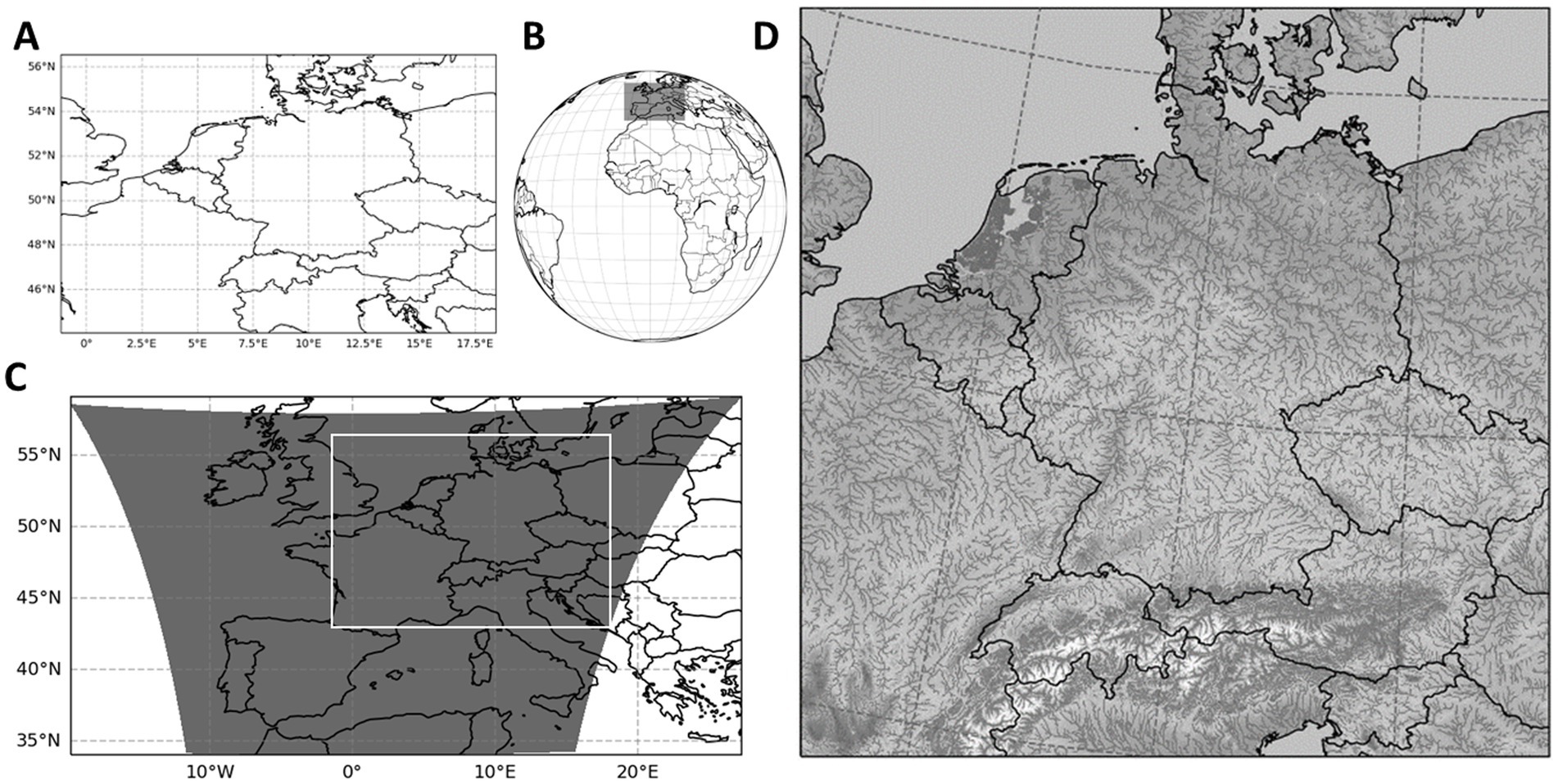
Figure 2. Study domain and grids of HRES (A), H-SAF (B), resampled and trimmed H-SAF (C) data, and DE06 grid (D). Maps shown on panels (A,C) are mapped in Plate Carree projection. Panel (B) is shown in geostationary (azimuthal) projection, and (D) is shown in EUR-11 rotated-pole projection as used in the DE06 setup.

Satellite-based data from H-SAF, P-AC-SEVIRI-PMW (referred to as H61B in this section and H-SAF throughout the rest of the manuscript) is an hourly accumulated precipitation dataset. H61B is derived by integrating Passive Microwave (PMW) sensor and SEVIRI (visible and infrared) instrument data. H61B improves prior H-SAF precipitation data by classifying rainfall as convective or stratiform through adjustments in the rain rate-brightness temperature relationship (EUMETSAT, 2021b, 2022). H61B data spans from latitude 60°S to 67.5°N and longitude 80°W to 80°E, and is rectified, projected, and resampled into a defined grid (Figure 2B). The spatial resolution is ~4.8 km at nadir, but it decreases in areas away from the nadir point, reaching ~8 km over Europe. To obtain H-SAF data for the first domain and grids, a reference algorithm by Mueller et al. (2018), is used to establish the relationship between the pixel locations to geographic coordinates. The data from the full disc area is trimmed for size reduction (Figure 2B), resampled to the 0.1° × 0.1° HRES grid using remapbil bilinear interpolation function (Figure 2C), and then trimmed to fit the study domain (Figure 2A). Resampling is necessary to match the input and output dimensions of the data for calculating the mismatches in corresponding grids required for the U-Net architecture.

The second grid definition (Figure 2D) has a resolution of 0.0055° × 0.0055° (∼0.611 km × 0.611 km) in the lateral direction, covering 2000 × 2000 grid cells. This grid extends over 15 terrain-following vertical model layers with increasing thickness from the land surface to the model bottom. The uppermost layer reaches from the surface to 2 cm depth and the lowest layer extends from 42 to 60 m below the surface. This is called the DE06 grid in the ParFlow/CLM setup, a high-resolution hydrological model that simulates the water and energy cycles in the study domain. For more information about the DE06 setup, the reader is referred to Belleflamme et al. (2023). All the precipitation data are remapped using remapbic bicubic interpolation function onto the DE06 grid (Figure 2D) to be used in ParFlow/CLM simulations.

2.3 Precipitation correction

2.3.1 DL network setup

We employ a Deep Learning (DL)-based framework introduced by Patakchi Yousefi and Kollet (2023). This approach relies on the non-linear space–time relationships between the extracted features from the input data, and the mismatch between the model-based HRES and H-SAF reference data. The framework consists of two steps (Equations 1, 2). First step is to learn the mismatch data:

\begin{array}{l} {D L}_{p r} (I_{p r, i, t}, w_{p r}) : I_{p r, i, t} \to δ_{p r, i, t}, where δ_{p r, i, t} = m_{p r, i, t} - r_{p r, i, t} & (1) \end{array}

where ${D L}_{p r} (I_{p r, i, t}, w_{p r})$ represents the DL network with inputs $I_{p r, i, t}$ to be trained on the mismatch data $δ_{p r, i, t}$ for precipitation $p r$ as a modeled $m_{p r, i, t}$ , and observed $r_{p r, i, t}$ atmospheric variable over time $t$ and location $i$ .

The second step is to remove mismatches from $m_{p r, i, t}$ using the trained weights in the network independent from observations:

\begin{array}{l} {\hat{m}}_{p r, i, t} = m_{p r, i, t} - {\hat{δ}}_{p r, i, t} & (2) \end{array}

where the corrected HRES precipitation (HRES-C) ${\hat{m}}_{p r, i, t}$ is obtained by removing the predicted mismatch ${\hat{δ}}_{p r, i, t}$ from the original modeled data $m_{p r, i, t}$ .

The U-Net architecture employed in this study for precipitation correction follows the work of Patakchi Yousefi and Kollet (2023), featuring a U-Net CNN (Ronneberger et al., 2015) with a distinct feature of squeeze-and-excitation (SE) blocks between the two convolutional functions both in the up-sampling and down-sampling steps. The SE blocks contain global average pooling followed by convolutional operations with relu and sigmoid activations. Global average pooling layer computes the average value of all feature maps for each batch and channel, summarizing the information into a single representative value. This map is reshaped and processed through two 1 × 1 convolutional layers. The SE blocks perform channel-wise attention, emphasizing informative features and suppressing less useful ones (Hu et al., 2019). The architecture incorporating the layers and blocks discussed above is illustrated in Figure 3.

Figure 3

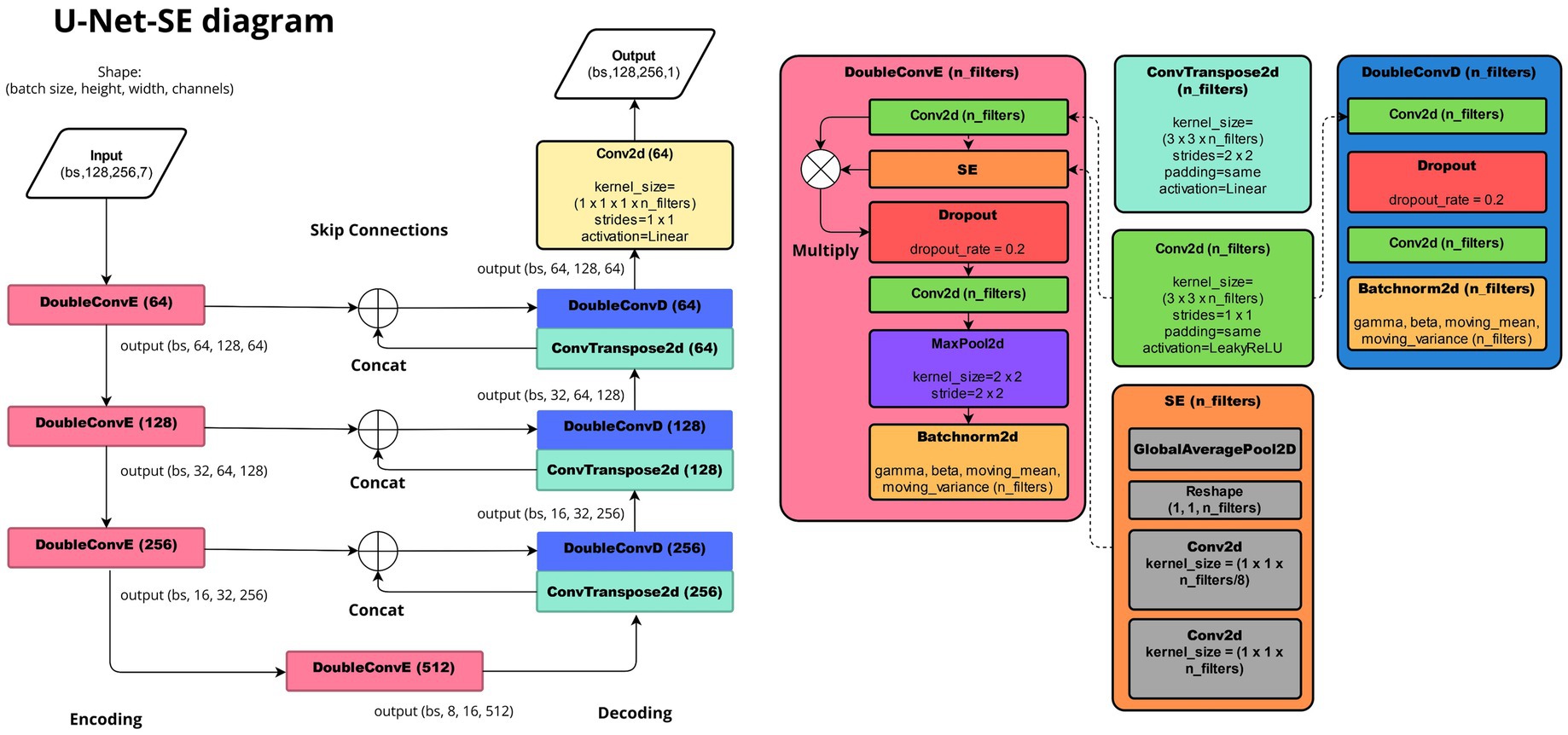
Figure 3. Schematic representation of the U-Net convolutional neural network architecture used in this study with Conv2d, SE, Dropout, MaxPool2d, Batchnorm2d, GlobalAveragePool2D, ConvTranspose2d, Concat, and Multiply layers from Keras library.

Previous similar studies emphasize including spatiotemporal information to improve U-Net predictions (Bastos et al., 2021; Teimouri et al., 2019). In our approach, we include a total of seven input channels. These channels include modeled precipitation data at $t$ and $t - 1$ , geographical coordinates (latitude and longitude), altitude maps and calendar information specifying year, and day of the year (assigned to all pixels in the corresponding image). Each input channel undergoes batch normalization layer (Keras library in python), immediately after the input layer to standardize each channel’s values by subtracting the batch mean and dividing by the square root of the batch variance. This normalization step ensures that all channels contribute effectively to the learning process by maintaining consistent scaling with trainable parameters. All corresponding input and target data with 196 × 125 dimension are filled with zero padding to obtain images with the nearest square dimensions of 256 × 128 for training in U-Net.

2.3.2 U-Net training

We employ and compare two loss functions: Mean Squared Error (MSE) and Weighted MSE (WMSE). We employ and compare two loss functions (Equations 3, 4):

\begin{array}{l} M S E_{T} = \frac{1}{N_{T} N_{S}} \sum_{t = 1}^{N_{T}} \sum_{i = 1}^{N_{S}} M_{land, i} M_{avail, i, t} {({\hat{δ}}_{p r, i, t} - δ_{p r, i, t})}^{2} & (3) \end{array}

where $M S E_{T}$ represents the loss during the training period; $N_{T}$ and $N_{S}$ represent the number of data points in time and space; $M_{land, i}$ and $M_{avail, i, t}$ represent binary masks for land and H-SAF data availability; ${\hat{δ}}_{p r, i, t}$ and $δ_{p r, i, t}$ represent the predicted and actual precipitation mismatches over location $i$ and time $t$ . $M S E_{V}$ $M S E_{T E}$ are similarly defined for validation data, as well. The MSE loss function is formulated to reduce the mean squared error between predicted and actual precipitation.

The WMSE loss function is defined as

\begin{array}{l} W M S E_{T} = \frac{1}{N_{T} N_{S}} \sum_{t = 1}^{N_{T}} \sum_{i = 1}^{N_{S}} W_{p r, i, t} M_{land, i} M_{avail, i, t} {({\hat{δ}}_{p r, i, t} - δ_{p r, i, t})}^{2} & (4) \end{array}

where $W M S E_{T}$ represents the weighted loss during the training period; $W_{p r, i, t}$ corresponds to the intensity weights calculated for each pixel $i$ and time $t$ over the training period. $W M S E_{V}$ $W M S E_{T E}$ are similarly defined for validation data, as well.

The WMSE loss function introduces intensity-based weighting to emphasize higher-intensity precipitation events. To calculate $W_{p r, i, t}$ , we obtain the probability of H-SAF precipitation categorized into three levels: dry (up to 0.1 mm/h), light (0.1 to 2.5 mm/h), and moderate to heavy (more than 2.5 mm/h). Toprioritize moderate to heavy over dry and light categories, we calculate the $W_{p r, i, t}$ for each category such that the sum of inversely weighted probabilities for each precipitation category equals to one. The calculated weights are presented in Table 1. Furthermore, in both loss functions, we utilize a stationary land and a dynamic data availability mask specifically to train the loss function over land grids where H-SAF data is accessible.

Table 1

Table 1. Probability of occurance (%) for each precipitation intensity over the training dataset for HRES, H-SAF and HRES-C.

2.3.3 Hyperparameter tuning

A simple hyperparameter tuning (HPT) is employed to optimize the performance of U-Net. The tuned parameters include initial learning rate (LR), batch size (BS), and the number of filters in the first U-Net network layer. The LR values tested are 0.01, 0.001, and 0.0001, the considered batch sizes are 2, 4, 8, and 16, and the number of filters in the first layer of the U-Net architecture is chosen from 8, 16, 32, and 64. The possibility of reaching an optimum result with a wider range of combinations is possible. However, the current selection of 48 different combinations is reasonable, given the computational resources required for more extensive search.

The study period for precipitation correction is between 2020-07-01 13UTC and 2023-04-25 12UTC. The data is randomly split 50/50 into training and validation sets. The validation set consists of multiple clusters of 10 consecutive days (240 h) within the study period with an equal duration of hours as the training set.

In HPT, the goal is to find the best combination of hyperparameters that result in better and robust skill in predicting mismatches, toward the final goal of improving HRES data. Therefore, for each parameter combination, and in each training epoch, model training is performed using the training set and validated with the validation set. If there is no improvement in validation loss after 8 epochs, the training is stopped (early stopping). If the validation loss does not improve after 2 epochs, the learning rate is reduced by a factor of 0.5. Following these runs, we analyze the results to identify the HPT combination that leads to the least validation loss and save it for producing the corrected HRES. The results from HPT are provided in Section 3.1.

2.4 ParFlow/CLM simulations

We employ the ParFlow v3.8.0 integrated hydrological model which utilizes partial differential equations (PDEs) to simulate variably saturated subsurface and groundwater flow, integrated with overland flow, which constitutes the upper boundary condition (Kollet and Maxwell, 2006; Kuffour et al., 2020; Maxwell et al., 2015). The physics-based methodology of ParFlow yields consistent results across time and space scales, ranging from watershed hydrodynamics to large-scale continental simulations (Maxwell et al., 2015; Saadi et al., 2023a). ParFlow can be run efficiently on large HPC systems, including GPUs (Burstedde et al., 2018; Hokkanen et al., 2021; Kollet et al., 2010).

In this study, the model uses the same setup with the same external parameter files for slopes, soil hydraulic properties, land cover, etc. as in the experimental forecasts runs by Belleflamme et al. (2023). The Community Land Model (CLM) in ParFlow/CLM, enhances the representation of energy and mass fluxes by adding land surface exchange processes such as interception and evapotranspiration (Kuffour et al., 2020). We use ParFlow/CLM model outputs from the aforementioned study from 2020-06-30 13UTC up to the next 24 h for our runs as the initial conditions. From 2020-07-01 13UTC and onwards, three different precipitation forcing data are tested with dedicated ParFlow/CLM model runs: H-RES, H-SAF, and corrected HRES (HRES-C). The model is run on the GPU compute nodes of the JUWELS Booster HPC system at the Jülich Supercomputing Centre.

2.5 Evaluation methods

To assess the fidelity of the precipitation data, we employ a variety of evaluation metrics at hourly and monthly time scales such as Mean Error (ME), Root Mean Squared Error (RMSE), and Pearson Correlation (COR). ME quantifies the overall bias against the reference data, indicating whether the predictions tend to overestimate or underestimate actual values. RMSE measures variability and magnitude of deviations from reference data. COR is utilized to indicate the strength and direction of the linear relationship between simulated (or predicted) and reference values. COR and RMSE metrics are also used to evaluate simulated SM. These metrics are calculated according to Patakchi Yousefi and Kollet (2023).

COR and RMSE metrics are used for comparing simulated against observed SM. Additionally, we evaluate the spatial patterns using the SPAEF multi-component metric that accounts for the spatial correlation, variability rate, and histogram match. For further details on the SPAEF metric, refer to Koch et al. (2018).

False Alarm Ratio (FAR) and Probability of Detection (POD) are utilized to evaluate the reliability of specific precipitation thresholds of 0.1, 2.5, and 10 mm/h by different datasets. FAR measures the ratio of falsely identified events above a threshold to the total number of identified events above that threshold. POD represents the proportion of correctly identified precipitation events above a specific threshold out of all events that exceeded that threshold. For more information regarding POD and FAR, the reader is referred to Amjad et al. (2020).

3 Results and discussion

In this section, we present and discuss key results from calculating the intensity weights in section 3.1, network hyperparameter tuning in Section 3.2, precipitation correction in Section 3.3, comparing SM simulations in Section 3.4, and validation of precipitation products in Section 3.5.

3.1 Intensity weights

The inverse intensity weights were calculated by first calculating the probability of occurrence for each precipitation category based on the H-SAF training dataset. The assigned weight is shown for each precipitation category.

3.2 Hyperparameter tuning

While exploring the efficacy of the loss function based on WMSE in HPT experiments, a marginal improvement (less than 1%), between the WMSE and the MSE was observed for both training and validation (not shown). Given the limited impact of the WMSE on overall model performance, we proceed with the MSE results in our subsequent analyses and discussion.

Figure 4A shows the training (solid colored lines) and validation (dotted colored lines) MSE loss over the training epochs for the top five HPT settings according to the validation loss. The remaining gray lines represent the rest of the experimented HPT settings. We found that larger initial filter numbers (IFN) and batch sizes (BS) contribute to a smaller training loss and validation loss (i.e., model robustness). The best HPT setting (LR = 0.001, BS = 16, LRF = 0.5, and IFN = 64) is shown with the blue line.

Figure 4

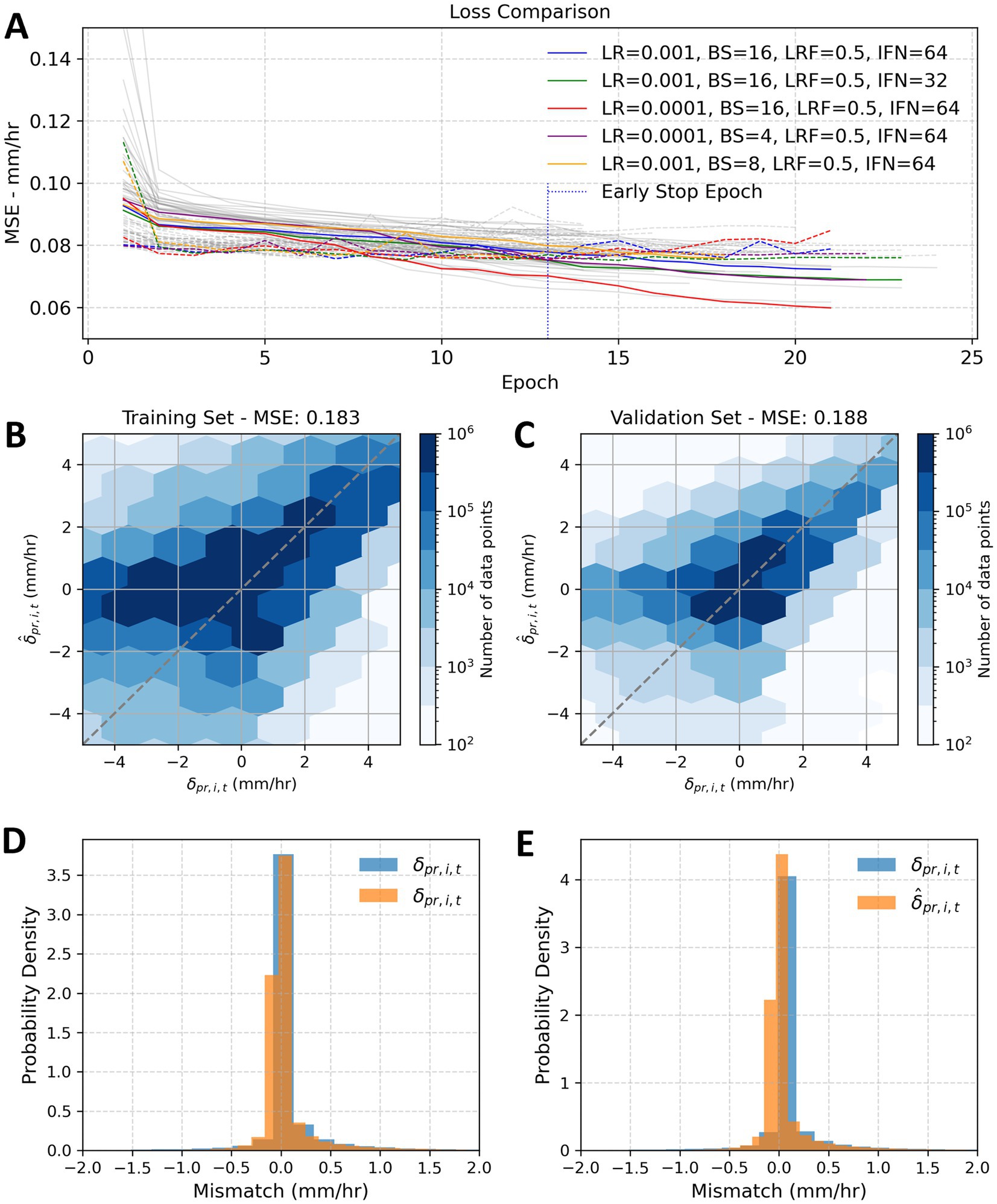
Figure 4. Training and validation loss comparisons for hyperparameter tuning (HPT) experiments for MSE loss function. Panel (A) shows the training and validation loss over training epochs for the top five HPT settings. Panels (B–E), respectively, represent the scatter and probability density function (PDF) diagrams for predicted ${\hat{δ}}_{p r, i, t}$ against actual $δ_{p r, i, t}$ data.

Figures 4B,C show the mismatch scatter diagram for actual $δ_{p r, i, t}$ against predicted ${\hat{δ}}_{p r, i, t}$ training and validation datasets. The consistency between the training and validation (in terms of predicting mismatch) sets is reflected by similar MSE values of 0.183 and 0.188 mm/h, respectively. Nevertheless, prediction skill is limited concerning negative mismatches (i.e., instances where HRES indicates low or zero precipitation) to be pronounced during seasons characterized by increased spatiotemporal variability, such as summer and fall, with increased likelihood of convective precipitation (Patakchi Yousefi and Kollet, 2023).

Figures 4D,E present the Probability Density Functions (PDFs) for mismatch data in the training and validation datasets, ranging from −2.0 to +2.0 mm/h. The distribution indicates a bias toward positive mismatches, because HRES generally forecasts higher precipitation rates than H-SAF observations. Overall, there is notable agreement between the actual and predicted mismatches, with the majority of the data concentrated between −1 and + 1 mm/h.

3.3 Precipitation correction

In the following, we further discuss our comparison results on the corrected HRES data (HRES-C) and the original HRES data against H-SAF between 2020-07-01 13UTC and 2023-04-25 12UTC. At this point, our assumption is that satellite-based precipitation (H-SAF) represents the reference. So, the better the agreement between HRES-C or HRES against H-SAF, the better the assumed precipitation accuracy.

Figures 5, 6 provide a spatiotemporal assessment of hourly error metrics, mean error (ME), root mean squared error (RMSE), and Pearson correlation (COR), across four seasons comparing HRES and corrected HRES-C data against H-SAF in the study region over the study period. Figure 5A illustrates the initial overestimation by HRES against H-SAF, depicting ME >0, while Figure 6A shows a post-correction improvement with ME ~0. Seasonal variations of RMSE are shown in Figures 5B, 6B, with increased error rates during the summer season, particularly in the southern regions corresponding to the Alps.

Figure 5

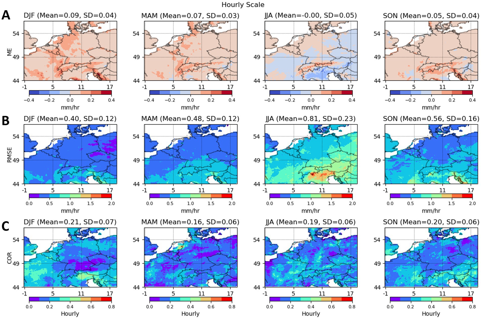
Figure 5. Maps of seasonal mean error (ME, A), root mean squared error (RMSE, B), and Pearson correlation (COR, C) metrics shown for HRES against H-SAF over four seasons in hourly scale.

Figure 6

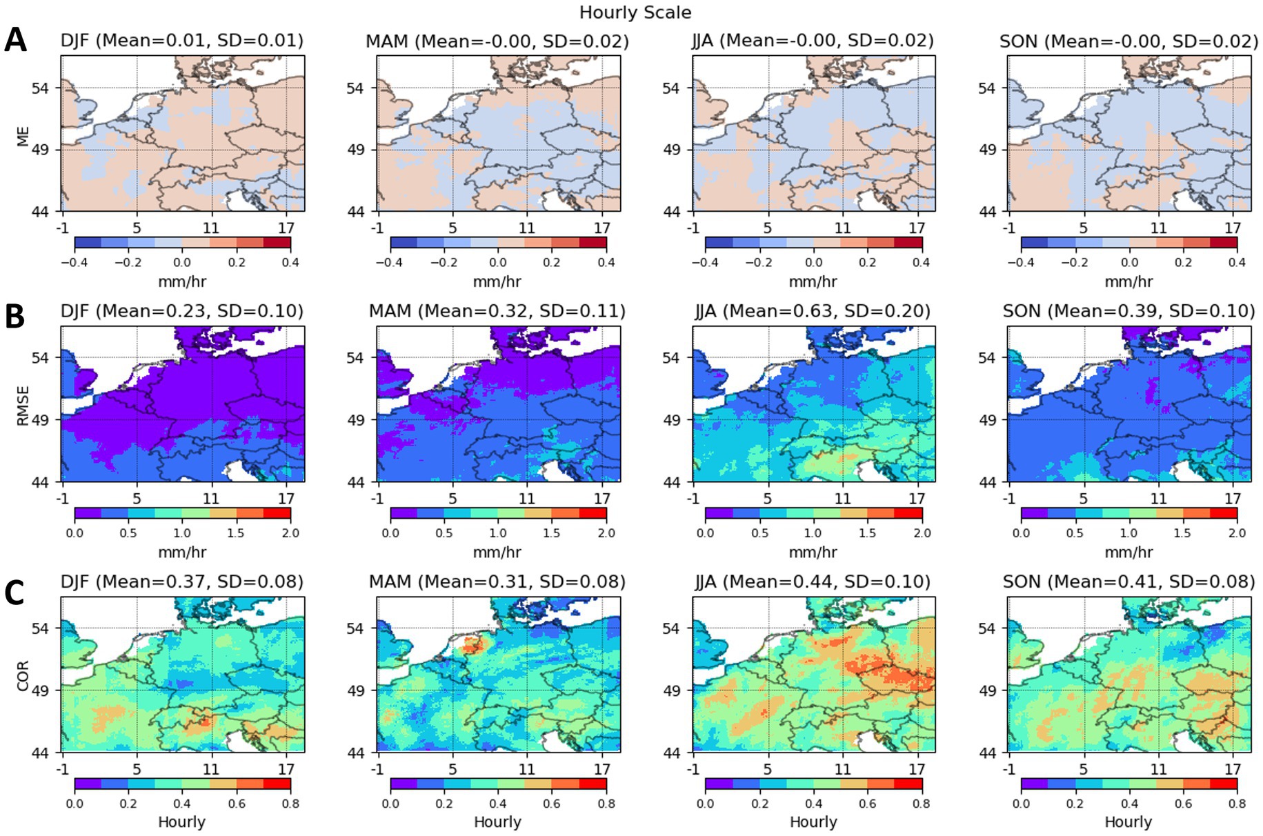
Figure 6. Maps of seasonal mean error (ME, A), root mean squared error (RMSE, B), and Pearson correlation (COR, C) metrics shown for HRES-C against H-SAF over four seasons in hourly scale.

Figure 7 presents maps illustrating the percent improvement achieved through the implementation of correction across four seasons as a quantitative comparison of alignment of HRES-C and HRES with respect to H-SAF, which is assumed as the ground truth. The average improvement in ME, RMSE, and COR is generally positive across all seasons when compared to H-SAF. An exception is observed in the summer season, where the average improvement in ME is negative. This discrepancy can likely be attributed to the presence of convective precipitation during summer, which tends to be more localized and intense, introducing uncertainties in both model- and satellite-based data.

Figure 7

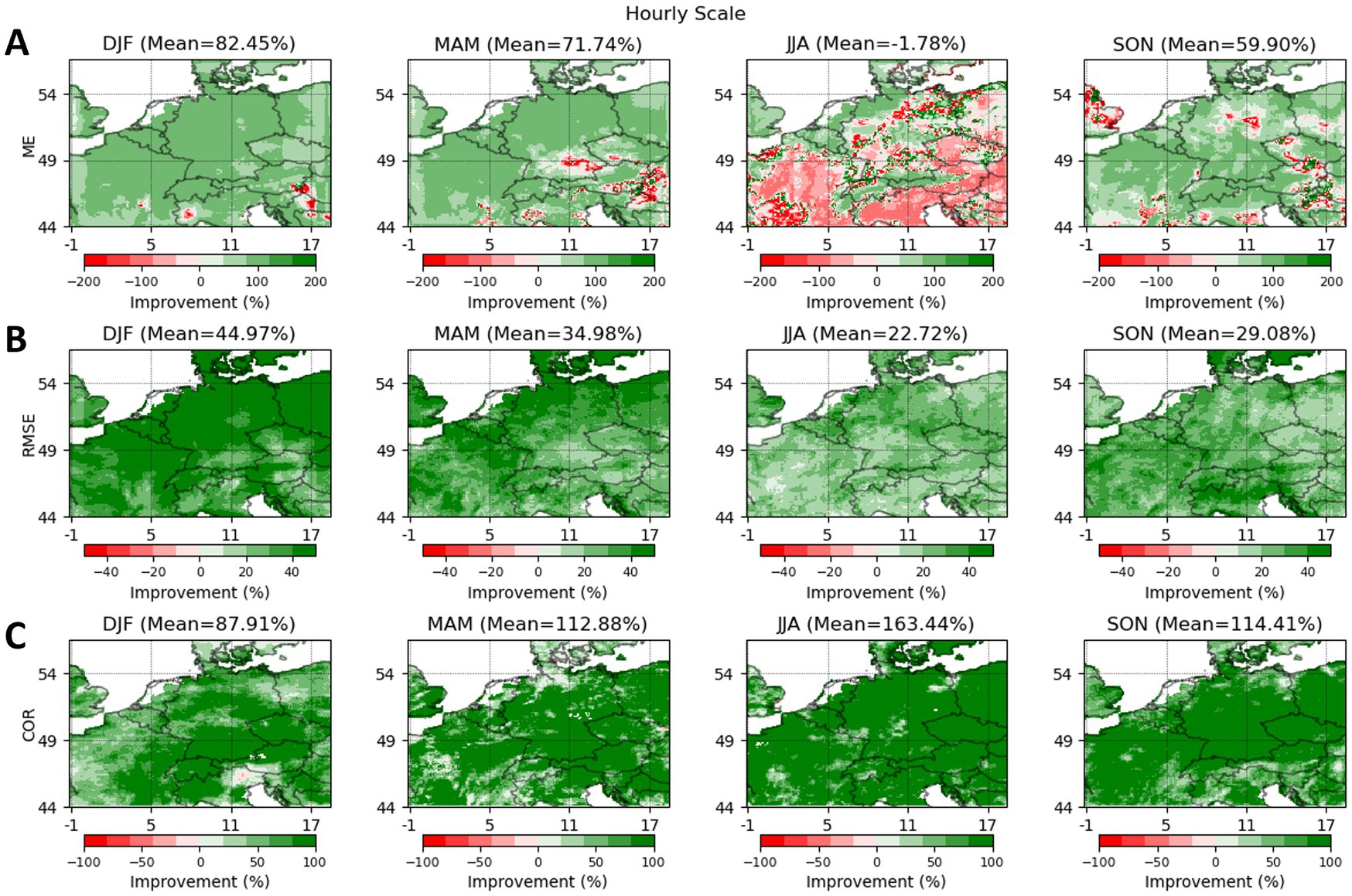
Figure 7. Maps of mean improvement [i.e., reduction in mean error (ME, A) and root mean squared error (RMSE, B) and increase in Pearson correlation (COR, C) in hourly scale] of HRES-C over HRES shown in percentage over four seasons.

3.4 Soil moisture simulations

Volumetric SM is used to study the impact of H-RES, H-SAF, and HRES-C precipitation forcing datasets on ParFlow/CLM simulations. To evaluate the accuracy and consistency of SM simulations, COR and RMSE metrics are used. The comparison is drawn against the ESA CCI SM data from 2020-07-01, to 2022-12-31, using daily and monthly values for comparison. For this, ParFlow/CLM data representing the uppermost soil layer (0–2 cm depth) are aggregated (averaged values of all nearest neighbor grids) to the coarser ESA CCI grid with a resolution of 0.25°.

The results depicted in Figure 8 surprisingly reveal that the SM simulations driven by the HRES 24 h forecast present lower RMSE and higher COR than those generated by satellite-based precipitation (H-SAF) or the corrected forecast (HRES-C). This unexpected outcome is particularly interesting considering the anticipated better agreement in SM simulations with ESA CCI through satellite-driven precipitation or DL-corrected forecasts. The existing 4D-Var assimilation scheme of HRES with a diverse array of observations, including in-situ and remotely sensed data, potentially establishes the reliability of the HRES 24 h precipitation forecast in representing SM dynamics as it appears to closely mirror the trends observed in ESA CCI SM data.

Figure 8

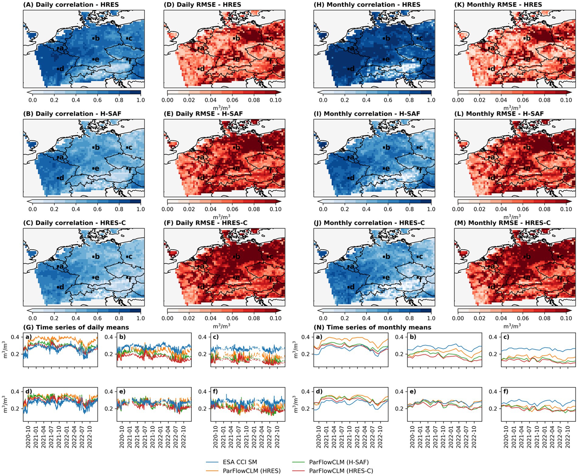
Figure 8. Comparison of daily (A–G) and monthly (H–N) uppermost 2 cm volumetric SM simulations obtained by H-RES, H-SAF and HRES-C precipitation datasets run by ParFlow/CLM against ESA CCI SM. Panels (A–C) and (H–J) show the distribution of correlation, and panels (D–F,K–M) show the distribution of root mean square error of SM values over the study area between 2020-07-01 and 2022-12-31. Panels (G,N) show the daily and monthly time-series of SM over six random locations (a–f) pinned on the study area.

Figure 8 reveals consistency in the patterns observed between H-SAF and HRES-C simulation outcomes across daily and monthly correlations, with a slightly better performance observed in the former dataset. This consistency highlights the effectiveness of the DL-based correction method in forcing SM simulations that closely mirror the SM driven by H-SAF dataset.

The HRES dataset shows the best overall SPAEF performance (Figure 9). Both HRES and H-SAF have similar histogram match ratios, but H-SAF shows a higher CV ratio, indicating greater variability mismatch and lower spatial COR, indicating less consistency in spatial patterns with ESA CCI SM data. While HRES-C dataset achieves the highest spatial COR, indicating accurate spatial pattern representation, it does not lead to an overall improvement in the SPAEF metric.

Figure 9

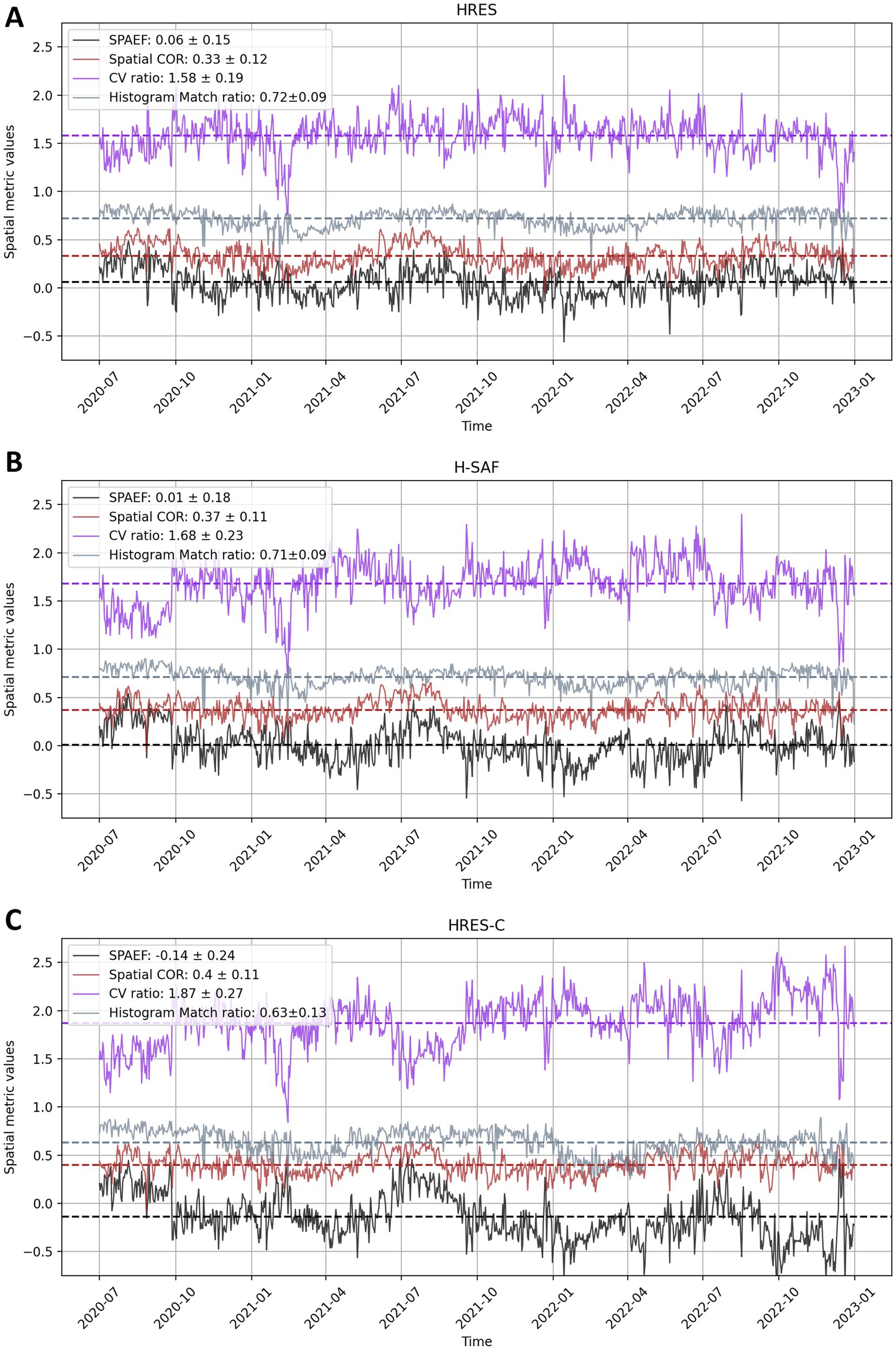
Figure 9. Daily time-series the spatial metrics for SM simulations using HRES (A), H-SAF (B), and HRES-C (C) precipitation datasets against ESA CCI SM. The metrics include the Spatial Efficiency (SPAEF) and its components: spatial Pearson correlation coefficient (spatial COR), coefficient of variation (CV) ratio, and histogram match ratio. The average values of the metrics are shown in mean ± standard deviation. In figure, we analyze the spatial performance of the SM simulations driven by the HRES, H-SAF, and HRES-C precipitation datasets using the Spatial Efficiency (SPAEF) metric and its components: spatial Pearson correlation coefficient (spatial COR), coefficient of variation (CV) ratio, and histogram match ratio. The SPAEF metric, ranging from −∞ to 1, quantifies the agreement between simulated and observed SM, where higher values indicate better spatial performance.

3.5 Precipitation data validation

In Section 3.2, the assessment reveals that HRES-C agrees well with H-SAF concerning ME, RMSE, and COR. However, as explored in Section 3.3, the alignment of SM simulations with observations (ESA CCI data) is not consistently improved. This discrepancy prompts a re-evaluation of the precipitation data using in-situ measurements (i.e., rain gauge station data), focusing on H-RES, H-SAF, and HRES-C, to understand the reasons for the observed gaps.

In the re-evaluation, 16 rain gauges were randomly picked across Germany with available data from July 2020 to the end of 2022 and located the nearest pixel from the precipitation datasets to the station locations. The monthly time-series of the three precipitation datasets and the rain gauge station data as well as H-SAF data quality index (QI) is provided in Figure 10A. Figure 10B shows the locations of these stations over the map of H-SAF mean data availability (mean ratio of available data during the study period) shown in percentage. Figure 10C shows the station locations over the map of mean QI provided by H-SAF metadata and averaged over the study period.

Figure 10

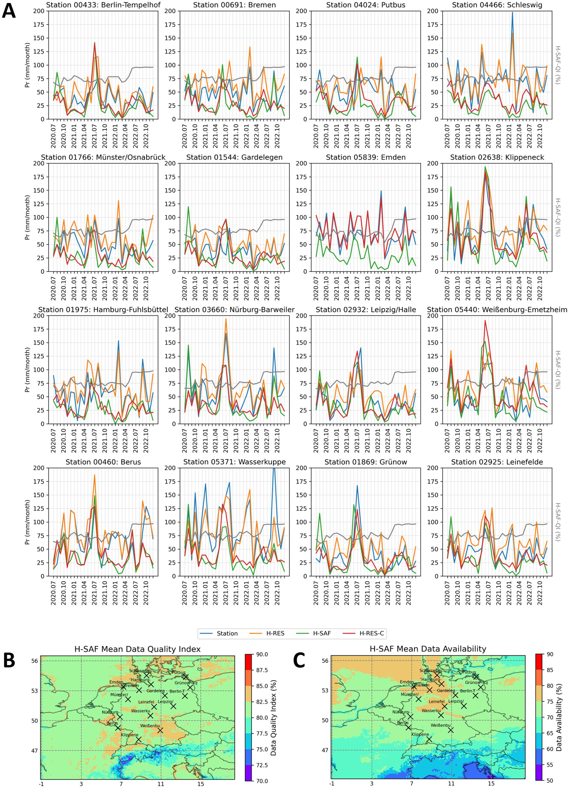
Figure 10. Comparison of H-RES, H-SAF, and HRES-C against rain gauge observations. Panel (A) shows time-series of monthly precipitation sum (mm/month) as well as average H-SAF quality index (QI) for 16 randomly selected rain gauge stations across the study domain from July 2020 to the end of 2022. Panels (B,C), respectively, show the maps of H-SAF data availability and quality index (H-SAF-QI) across the study domain. Locations of randomly selected rain gauge stations are pinned over the maps.

According to Figure 10A, the monthly sum of precipitation obtained by HRES-C generally matches H-SAF, resembling our findings in downstream simulations (Figure 8). However, HRES demonstrates a better agreement with rain gauge data. H-SAF underestimates precipitation compared to the rain gauge data, in line with findings from a validation report noting a slight underestimation in all precipitation classes for the H61B H-SAF product (EUMETSAT, 2022).

The H-SAF Quality Index (QI) steadily increases from March to July 2022, indicating improved data reliability during this period (see the gray lines over time-series in Figure 10A). The mean QI is calculated over all station locations and compared against the COR in Figure 11A as well as mean RMSE and ME in Figure 11B. There seems to be a positive relationship between the reduction in absolute ME and COR as well as increment in RMSE and the mean QI of each station. Therefore, the quality and accuracy of HRES-C could potentially be attributed to errors and uncertainties in H-SAF both before and after July 2022. While assessing changes in performance post-July 2022 is possible by training the network after this date and evaluating the changes in performance, this is out of the study’s scope.

Figure 11

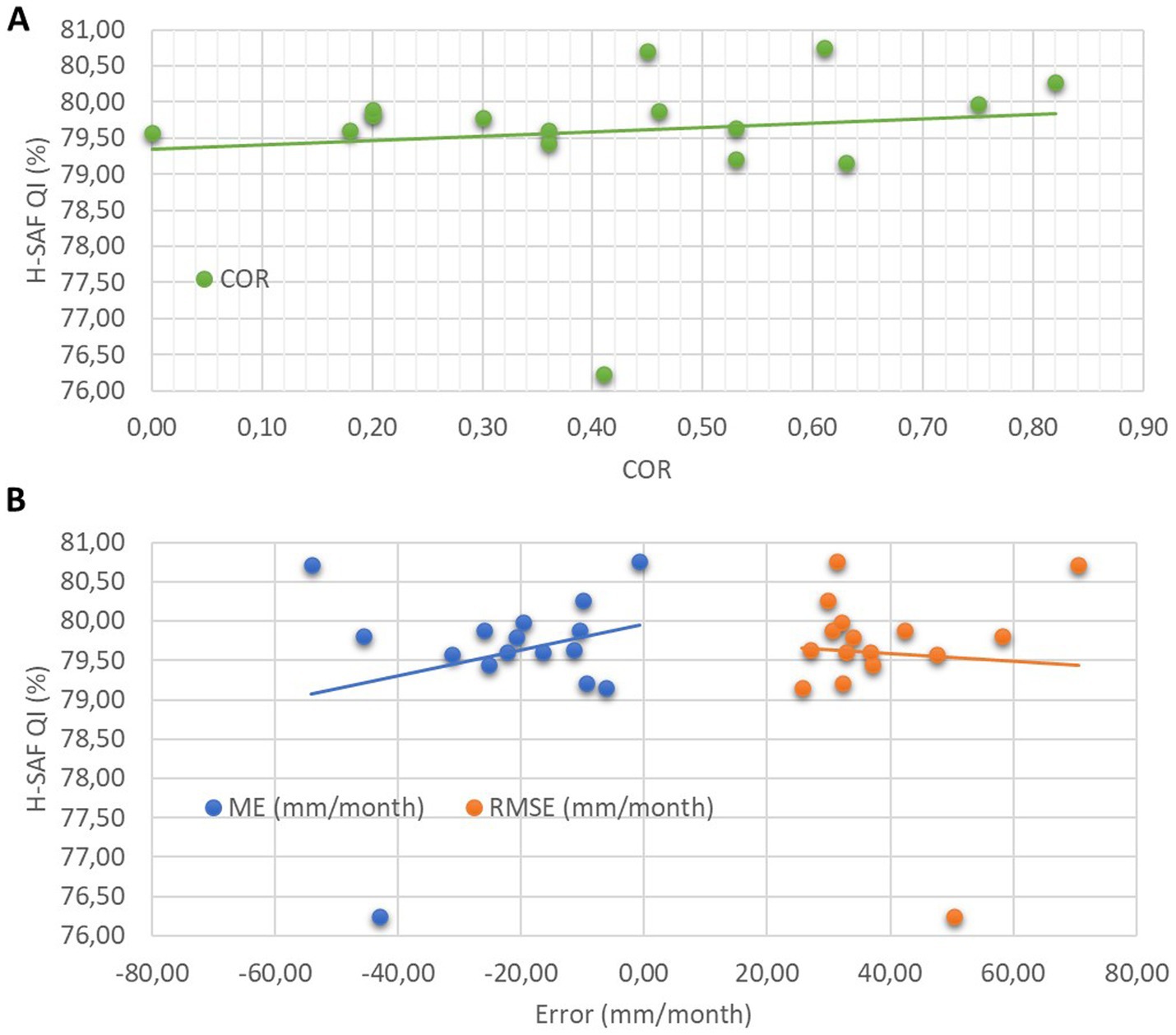
Figure 11. Scatterplots representing the relationship between average H-SAF QI (%) and COR (A) as well as ME and RMSE (B) over 16 rain gauge stations.

Figure 12 and Table 2 provide an evaluation of hourly error metrics for H-RES, H-SAF-O, H-SAF, and HRES-C. H-SAF-O represents H-SAF data without preprocessing to account for its effects of trimming and remapping on HRES domain and grids. In comparison, HRES demonstrates better performance with lower ME (in absolute value), reduced RMSE, and higher COR against the 16 randomly chosen rain gauge stations.

Figure 12

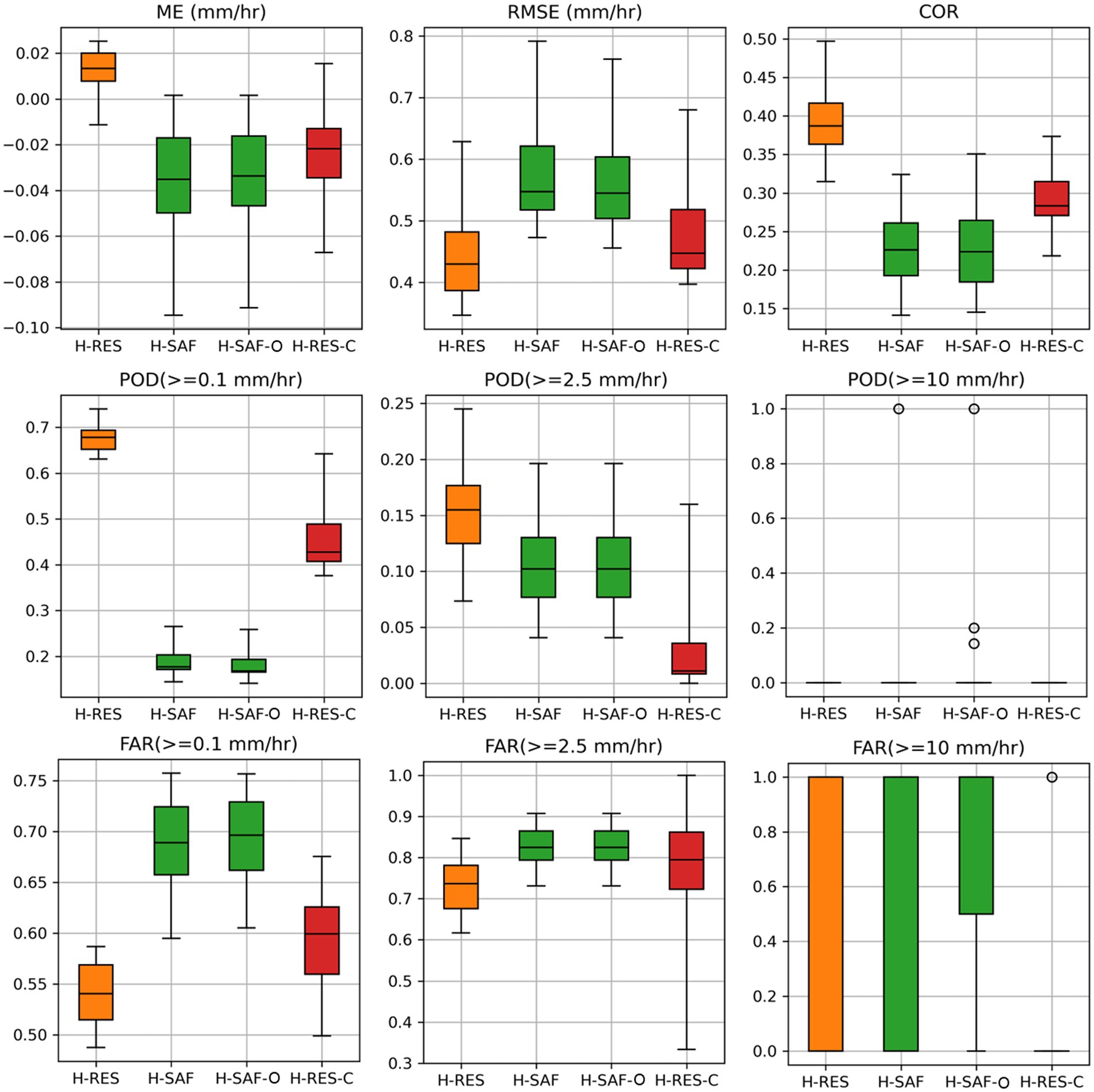
Figure 12. Boxplot comparison of H-RES, H-SAF, H-SAF-O, and HRES-C against rain gauge observations. H-SAF-O is the non-preprocessed H-SAF data used to account for the effect of preprocessing the data on evaluation results. POD and FAR, respectively, represent the probability of detection and false alarm ratio for three precipitation rates.

Table 2

Table 2. Overall hourly error metrics for H-RES, H-SAF, H-SAF-O, and HRES-C precipitation data presented as mean ± standard deviation.

Preprocessing H-SAF grid-wise to align with HRES exhibits slightly, but not significantly, higher ME and RMSE and a lower COR than H-SAF-O. Moreover, HRES-C shows improvements over both H-SAF and H-SAF-O, showing better metrics in ME, RMSE, COR, and POD of more than 0.1 mm/h.

For light precipitation events (POD > = 0.1 mm/h), HRES exhibits the highest detection rate, followed by HRES-C, while H-SAF and H-SAF-O show significantly lower POD. In terms of moderate precipitation (POD > = 2.5 mm/h), HRES shows higher detection, while the other products have lower detection rates. None of the products effectively detect high-intensity precipitation events (POD > = 10 mm/h). Regarding FAR, HRES and HRES-C have lower false alarm rates for light and moderate precipitation compared to H-SAF and H-SAF-O. For high-intensity events, HRES-C stands out with the lowest FAR, indicating a much lower rate of false alarms compared to H-SAF and H-SAF-O.

4 Conclusion

In this study, we evaluated the immediate and downstream impacts of implementing U-Net CNN DL-based correction on HRES precipitation using the satellite-based H-SAF h61 precipitation observations toward operational hydrological simulations over central Europe. The findings of this study highlight the effectiveness of using the DL-based precipitation correction in improving the accuracy of precipitation forecast. The corrected precipitation data (HRES-C) exhibited greater agreement in mean error, root mean squared error, and correlation with the assumed reference data (H-SAF), compared to the forecast data (H-RES). This shows the potential of DL-driven methods in correcting precipitation data despite the data imbalance of hourly precipitation and spatiotemporal gaps in satellite-based data.

For soil moisture (SM) simulations, the HRES 24-h forecast used as forcing data shows greater spatiotemporal agreement with the referenced ESA CCI SM data compared to both H-SAF and HRES-C. The additional evaluation of these three datasets against 16 rain gauge data supports these findings with higher consistency of HRES with the rain gauge observations compared to the other datasets. This highlights the importance of reference data quality in DL-based correction approach and challenges the assumptions on the better representativity of H-SAF satellite-based observations as ground truth for short-term correction or near real-time application in operational hydrological forecasting.

Future research should focus on the limitations related to deterministic aspects in DL-based correction methods, e.g., to account for uncertainties in the reference data. Furthermore, the accuracy of forecast data is expected to diminish over time, particularly as the forecast lead time extends. We focused on implementing the correction over the initial 24-h forecast from H-RES. Yet, we recognize the potential for improvements in longer-term forecasts.

Code and data availability

The preprocessed data of this article is made available by the authors (Patakchi Yousefi et al., 2024). The codes regarding the data preprocessing, precipitation correction, and post-processing of forcing data can be found at https://gitlab.jsc.fz-juelich.de/kiste/atmoscorrect. ParFlow/CLM documentation and codes are publicly available at https://parflow.org/.

Data availability statement

The original contributions presented in the study are included in the article/supplementary material, further inquiries can be directed to the corresponding author.

Author contributions

KP: Conceptualization, Data curation, Formal analysis, Methodology, Resources, Software, Validation, Visualization, Writing – original draft, Writing – review & editing. AB: Conceptualization, Formal analysis, Software, Visualization, Writing – review & editing. KG: Conceptualization, Data curation, Formal analysis, Funding acquisition, Methodology, Project administration, Resources, Software, Supervision, Writing – review & editing. SK: Conceptualization, Data curation, Formal analysis, Funding acquisition, Investigation, Methodology, Project administration, Resources, Software, Supervision, Validation, Visualization, Writing – review & editing.

Funding

The authors declare financial support was received for the research, authorship, and/or publication of this article. We acknowledge receive funding through the BMBF BiooekonomieREVIER funding scheme with its “BioRevierPlus” project (funding ID: 031B1137D/031B1137DX). Furthermore, we gratefully acknowledge the AI Strategy for Earth System Data (KI:STE) and Earth System Modeling (ESM) projects for funding this study by providing computing time the supercomputer JUWELS at Jülich Supercomputing Centre (JSC).

Acknowledgments

We thank the ECMWF for providing free access to their weather forecasts, EUMETSAT for satellite observations, Deutscher Wetterdienst (DWD) for rain gauge observations, and ESA CCI for soil moisture data. We also acknowledge the use of OpenAI’s ChatGPT versions 3.5 and 4 as a tool in initializing the first draft of this manuscript. Finally, we appreciate the constructive suggestions by the reviewers, which greatly contributed to the improvement of this manuscript.

Conflict of interest

The authors declare that the research was conducted in the absence of any commercial or financial relationships that could be construed as a potential conflict of interest.

Publisher’s note

All claims expressed in this article are solely those of the authors and do not necessarily represent those of their affiliated organizations, or those of the publisher, the editors and the reviewers. Any product that may be evaluated in this article, or claim that may be made by its manufacturer, is not guaranteed or endorsed by the publisher.

References

Amjad, M., Yilmaz, M. T., Yucel, I., and Yilmaz, K. K. (2020). Performance evaluation of satellite- and model-based precipitation products over varying climate and complex topography. J. Hydrol. 584:124707. doi: 10.1016/j.jhydrol.2020.124707