- 1Laboratory of Mathematics, Statistics and Applications, Faculty of Sciences, Mohammed V University, Rabat, Morocco
- 2Department of Mathematics and Statistics, Université de Moncton, Moncton, NB, Canada
This research paper explores the implementation of machine learning (ML) techniques in weather and climate forecasting, with a specific focus on predicting monthly precipitation. The study analyzes the efficacy of six multivariate machine learning models: Decision Tree, Random Forest, K-Nearest Neighbors (KNN), AdaBoost, XGBoost, and Long Short-Term Memory (LSTM). Multivariate time series models incorporating lagged meteorological variables were employed to capture the dynamics of monthly rainfall in Rabat, Morocco, from 1993 to 2018. The models were evaluated based on various metrics, including root mean square error (RMSE), mean absolute error (MAE), and coefficient of determination (R2). XGBoost showed the highest performance among the six individual models, with an RMSE of 40.8 (mm). In contrast, Decision Tree, AdaBoost, Random Forest, LSTM, and KNN showed relatively lower performances, with specific RMSEs ranging from 47.5 (mm) to 51 (mm). A novel multi-view stacking learning approach is introduced, offering a new perspective on various ML strategies. This integrated algorithm is designed to leverage the strengths of each individual model, aiming to substantially improve the precision of precipitation forecasts. The best results were achieved by combining Decision Tree, KNN, and LSTM to build the meta-base while using XGBoost as the second-level learner. This approach yielded a RMSE of 17.5 millimeters. The results show the potential of the proposed multi-view stacking learning algorithm to refine predictive results and improve the accuracy of monthly precipitation forecasts, setting a benchmark for future research in this field.
1 Introduction
The effects of climate change on water resources are increasingly important and concern various aspects of life in many countries. Studies on the impacts of climate change have gained great importance in recent years (Krysanova et al., 2017; Zhang et al., 2018; Wunsch et al., 2022). The objective is to comprehend the alterations in climate patterns (Trenberth, 2011; Liu et al., 2022; Verma et al., 2023; Gohil et al., 2024) and their consequences on water availability for future climates (Näschen et al., 2019). Several countries are experiencing severe climate conditions, and the least-developed countries are facing the most significant impacts. The IPCC’s 2022 report highlights its widespread implications for vulnerable populations, specifically in Africa (Parmesan et al., 2022). The severity and frequency of changes vary across regions. For example, some arid regions will experience extended periods of drought, while others may be affected by high levels of precipitation (Ahsan et al., 2022; Javan and Movaghari, 2022). Consequently, the prediction of climatic variables should consider these variabilities.
Climate change has significantly impacted Morocco’s development, especially in the agricultural sector, which contributes significantly to Morocco’s Gross Domestic Product (GDP), making it acutely vulnerable to climate shifts. Changes in precipitation patterns are among the major concerns of Moroccan scientists, as they affect water resource management, agricultural activities, and flood mitigation (Mehta et al., 2023). Accurate precipitation forecasts are crucial; however, they are becoming increasingly challenging due to climate change and human actions (Patel et al., 2024). Rainfall is recognized to be one of the most complicated variables to forecast in the hydrological cycle (e.g., Zounemat-Kermani et al., 2021; El Hafyani and El Himdi, 2022) due to the dynamic nature of environmental parameters and random fluctuations, both in terms of space and time. As a result, efforts have been made to reduce this non-linearity, employing techniques like wavelet analysis, singular spectral analysis, and empirical mode decomposition (Bojang et al., 2020). The mathematical and statistical models applied, however, call for very considerable processing power and can be time-consuming with little return (Singh and Borah, 2013). The emergence of wireless technologies, which sped up the development of affordable and effective methods for acquiring satellite images and historical radar data, was one factor that significantly contributed to the widespread use of ML in this field. Different studies indicate that ML-based models can be employed to identify nonlinear systems in multiple engineering sectors and can be applied in precipitation forecasting (Hung et al., 2009; Abhishek et al., 2012; Kumar et al., 2023).
It is essential to produce a precipitation forecast that is more reliable and easily comprehensible. Currently, meteorological prediction studies are increasingly incorporating artificial intelligence, like ML and neural networks. The findings of the research exhibit the high accuracy of prediction of precipitation, storms, and droughts for both short-term and long-term periods (Huntingford et al., 2019). ML can be categorized into two principal classifications. The first is “classical” techniques like multivariate linear regression (MLR), RF, KNN, support vector machines (SVM), and artificial neural networks (ANN). The second category is recognized as deep learning methods such as convolutional neural networks (CNN) and LSTM. Deep learning algorithms are widely used among short-term data sets; they generally call for large data sets to avoid overfitting. The use of time series models like LSTMs to take into consideration the time dimension of the data is usually recommended. Input factors in these models can comprise time lags (e.g., Dash et al., 2018; Danandeh Mehr et al., 2019; Kumar et al., 2019; Bojang et al., 2020) or geophysical features such as temperature, humidity, wind speed, and air pressure (Garg and Pandey, 2019; Baudhanwala et al., 2024). Various metrics are proposed with respect to the nature of the problem to evaluate the efficiency of ML models. As each study employs its own data sets, parameters, and pre-processing, it is practically impossible to proceed to a direct comparison of these results across multiple studies. However, some ML algorithms are most frequently mentioned as being better performers. Garg and Pandey (2019) forecast the rainfall using support vector regression (SVR), SVM, and KNN machine learning algorithms. They show that SVM proves to be the most effective in predicting rainfall. Other studies concluded that the multiple linear regression machine-learning algorithm was highly effective in predicting rainfall using dependent weather-related variables like temperature, humidity, moisture content, and wind speed (Balan et al., 2019; Gnanasankaran and Ramaraj, 2020). They show that the use of deep learning models could further improve the accuracy of rainfall prediction Tharun et al. (2018) performed the accuracy measurement to compare statistical modeling and regression algorithms (SVM, RF, and DT) for predicting rainfall using environmental variables. Results indicate that regression algorithms are more efficient at predicting rainfall than statistical modeling. The experimental findings demonstrated that the RF model outperformed and made more accurate predictions than the SVM and DT.
Wang et al. (2021) incorporated the MultiLLR machine learning model to forecast precipitation 2–6 weeks in advance, employing 21 climatological predictors. Pressure and Madden-Julian Oscillation are indicated to be the most potential variables, with varying predictive skills in different seasons. The study illustrates that incorporating supplementary factors such as the Arctic Oscillation and Western North Pacific Monsoon indices can improve the precision of predictions. According to Chhetri et al. (2020), several ML methods were used to predict the monthly rainfall in Bhutan. These included linear regression, multi-layer perceptron, CNN, LSTM, gated recurrent unit, and bidirectional LSTM. Among the six models, the LSTM model reached a first-rate mean square error (MSE) value of 0.0128. However, the proposed combination of BLSTM and GRU layers outperformed the other models, resulting in a significantly better MSE score of 0.0075, which was 41.1% better than LSTM. Moreover, this model also exhibited a stronger correlation value of 0.93. Chen et al. (2022) explored using a deep-learning-based LSTM model to predict monthly rainfall data. They evaluated its efficiency by comparing it with a RF data-driven approach. The authors use various window sizes to find the optimal lag times for the rainfall time series data. They assess the performance of the models using five statistical metrics and two visual means, namely Taylor and violin diagrams. Results show that the LSTM model outperforms the RF model in terms of rainfall prediction, demonstrating a notable enhancement in root mean square error (RMSE).
Stacking methods have not been extensively utilized in rainfall prediction. This technique is a specific type of ensemble method where the outputs of multiple base models are used as input to a higher-level “meta-model” to make the final prediction. This allows the meta-model to learn from the strengths and weaknesses of the base models and generate a more reliable prediction. Recent studies highlight the growing use of stacking methods in rainfall prediction. For instance, Gu et al. (2022) integrated four distinct ML algorithms: KNN, XGB, SVR, and ANN as their base models. This model is distinctive for its exploitation of a diverse set of predictors, such as climatic indices and local meteorological data. The findings from this study demonstrated that the utilization of a stacking strategy significantly boosts the predictive performance of the individual models, especially in spring and winter, underscoring the method’s potential to adjust to seasonal variability in rainfall patterns effectively. Similarly, Zandi et al. (2022) focused on the comparison of the performance of a stacked generalization ensemble approach with a locally weighted linear regression (LWLR) algorithm in estimating high-resolution monthly precipitation. Their ensemble model combines a multilayer perceptron neural network (MLP), SVM, and RF through a meta-learning algorithm. The stacking model demonstrates superior performance over both the best individual models, RF and LWLR, in terms of MAE, RMSE, and relative bias (rBias).
Predicting rainfall is a critical factor for agriculture in the Indian region. A novel stacking ensemble model has been introduced integrating various machine learning algorithms, including linear regression, RF, logistic regression, XGBoost, and SVR, with a second-layer learner synthesizing the predictions from these base models to generate more accurate rainfall forecasts. The research demonstrates a significant increase in predictive performance, achieving a maximum accuracy of 81.2%. This underscores the capacity of hybrid models to enhance the accuracy of rainfall prediction, indicating that such approaches can provide a versatile and adaptable framework for forecasting in different climates.
To our knowledge, unlike stacking techniques, multi-view stacking (MVS) learning has not yet been explored in precipitation forecasting. Multi-view learning focuses on constructing models from different “views” of the data. This approach assumes that each view can sufficiently train a good classifier, provided that the views are conditionally independent given the target class. One of the earliest works in this direction is the one by Blum and Mitchell (1998), which was developed primarily for semi-supervised learning tasks. Garcia-Ceja et al. (2018) and Van Loon et al. (2020) employed it lately in the context of supervised learning to enhance the performance of classification tasks. Nonetheless, this technique also holds potential for application in regression scenarios, particularly in our context of multivariate time series. This study marks a significant advancement in the accuracy of rainfall prediction. While previous studies have explored the prediction of monthly precipitation patterns, our research introduces a variety of innovative insights. The paper’s key contributions encompass:
1. The primary aim of our work is to assess and compare the performance of multiple ML techniques in the task of predicting monthly rainfall in Morocco. These techniques include DT, RF, AdaBoost, XGBoost, KNN, and LSTM.
2. The study intends to improve the accuracy of the predictions with the use of the innovative MVS technique, which allows for a more comprehensive understanding of the complex interactions among different “view” or meteorological factors and their impact on precipitation, ultimately resulting in more accurate rainfall forecasts.
3. Our adaptation of the novel technique of multi-view learning stacking, originally developed for classification purposes, to our context of multivariate time series regression is a unique contribution that has not been explored in previous machine learning research on this dataset.
4. The incorporation of lagged meteorological variables using the cross-correlation function (CCF) to identify the most relevant variables utilized as inputs for various ML models. These include lagged values for precipitation, maximal and minimal temperatures, and insolation, which are pivotal in understanding the temporal dynamics influencing rainfall patterns.
5. The findings of this study will serve as a baseline for subsequent investigations into rainfall prediction. Furthermore, this study is the first to apply advanced machine learning techniques, specifically multi-view stacking learning, to rainfall prediction in Rabat. This study offers valuable insights into the region and highlights the potential impacts of climate change on local precipitation patterns.
Our research not only fills a critical gap by providing valuable regional insights but also emphasizes the importance of regional climate studies to inform more nuanced and effective policy responses, both locally in Rabat and in similar urban contexts globally, where accurate prediction and understanding of rainfall patterns are crucial for sustainable urban planning and climate resilience.
The paper is structured as follows: The weather data set and the pre-processing steps taken to prepare it for experimentation are described in detail in the next section, which also provides an overview of six prediction models (DT, RF, KNN, AdaBoost, XGBoost, and LSTM) and the MVS learning technique, the hyperparameter optimization process, and the evaluation metrics used. Section 4 discusses the analytical and empirical outcomes. The final section concludes the work, summarizes the findings, and offers suggestions for future insights.
2 Materials and methods
2.1 Data and context description
Morocco’s diverse climatic regions are attributed to its geographical position in North Africa and the presence of a mountain range running from north-east to south-west, with altitudes up to 4,000 meters. The North Atlantic circulation has a significant impact on the climate of Rabat’s northwest coast, which is the wettest region in Morocco. The study area is Rabat, the capital of Morocco (Figure 1). It is located on the edge of the Atlantic, in the northwest of Morocco. It experiences a Mediterranean climate with noticeable seasonal variations (Brahim et al., 2016). Rabat has faced the impacts of climate change. These consequences incorporate increasing temperatures, more irregular rain patterns, and a rising risk of severe climatic events like intense rainfall, storms, and flooding. Figure 2 illustrates the seasonal precipitation variation in Rabat, with a significant concentration of rainfall occurring between November and March, peaking in December. This pattern is primarily due to Rabat’s position at the southern edge of frontal storm systems that regularly traverse the North Atlantic and southwest Mediterranean regions. For further details on the region’s climatology, refer to Driouech et al. (2021) and Tramblay et al. (2021). The persistence of the climate conditions and their effects on the rainfall dataset for Rabat will be analyzed through ML algorithms. A brief description of the proposed algorithms is given in the following section.
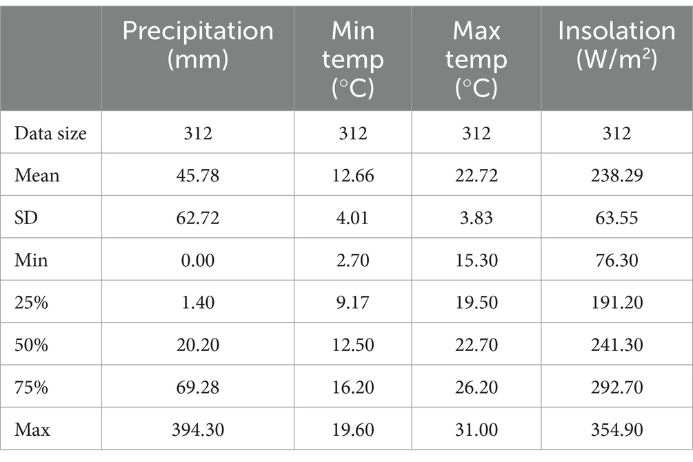
The research involves monthly rainfall records collected by the Moroccan General Directorate of Meteorology. The data set represents a multivariate time series that describes the monthly rainfall over 26 years, from 1993 to 2018, in Rabat. It comprises four variables: minimum temperature, maximum temperature, sunshine, and the target variable, which is rainfall. To evaluate the models, the first 24 years of data, from 1993 to 2016, were utilized as the training set. The last 2 years, covering 2017 and 2018, serve as the test set. The climatic variables considered in the study are detailed in Table 1, along with their main statistical characteristics. They include mean, standard deviation, minimum, and maximum values, in addition to values at the 25, 50% (median), and 75% percentiles. These measurements are interesting for understanding the variation and distribution of meteorological variables that are used as predictors of precipitation. Rainfall values span from 0 mm to 394.3 mm, with a mean of 45.78 mm and a high standard deviation of 62.72, indicating considerable variety in rainfall totals. Minimum temperatures range from 2.7 to 19.6°C, exhibiting a wide range of minimum temperatures, with a mean minimum temperature of 12.66°C and a standard deviation of 4.01. Maximum temperatures vary from 15.3 to 31°C, showing moderate fluctuations in this variable, with a mean of 22.72°C and a standard deviation of 3.83. Insolation values vary from 76.3 to 354.9 W/m2, illustrating a considerable range of solar energy exposure, with a mean insolation of 238.29 W/m2 and a standard deviation of 63.55, revealing a significant range in insolation levels.
The first step in using any ML technique is to prepare the raw data to make it suitable for model training and testing. Figure 3 depicts the pipeline of data preprocessing. To handle missing values in selected features, the mean of all values for the corresponding precipitation amount was calculated and used to estimate the missing values. For example, if there was a missing value for sunshine, the mean of other sunshine values with the same precipitation amount is used as an estimation. Then, the most relevant attributes that capture the variability of the data set are selected. To identify the most significant features, the cross-correlation function (CCF) is calculated to investigate the lag-time effects on the relationships between monthly precipitations and the meteorological variables. It quantifies the similarity between two series based on the lag between them. The time series data needs to be preprocessed to ensure stationarity; this step is crucial for using the CCF. Finally, the weather parameters are normalized using a min-max scale to obtain the new-scaled value y, as shown in Equation (1)
Where and are, respectively, the minimum and maximum values of as shown in Equation (1).
After completing the pre-processing step, the data is reshaped into a tensor representation that is compatible with the requirements of the LSTM layer. This transformation ensures that the input data takes on a 3D structure, including three distinct dimensions: samples, time steps, and the sample dimension.
2.2 Machine learning models
In this section, we will explore the ML models employed for predicting monthly rainfall patterns in Rabat. Various techniques are investigated, including DT, RF, KNN, AdaBoost, XGBoost, and LSTM. These supervised learning algorithms can handle both classification and regression tasks, offering broad applicability across numerous predictive modeling contexts. Each of these models has distinguishing characteristics and particular areas of application, providing researchers with the flexibility to select the most appropriate method for their specific issue.
2.2.1 Decision tree
A decision tree is a powerful predictive modeling tool widely used in machine learning, where predictions are presented in the form of a tree-structured classifier (Esposito et al., 1997). Decision trees are constructed by an algorithmic process that operates by recursively dividing the input feature space into subsets, each associated with a particular class label or predicted value. The main components of DT are internal nodes, which represent the features of a dataset, the branches connecting them represent the decision rules, and leaf nodes indicate the output of those decisions and do not have any further branches. This process iterates, applying decision rules at each node based on a feature’s value to split the dataset into two or more subsets, until achieving specific stopping criteria, such as a maximum tree depth or a minimum number of samples per leaf.
The main strengths of DT are its ability to handle both numerical and categorical variables, its resilience to outliers and missing values, and its strong skills in capturing nonlinear interactions and relationships within the data. Yet, DT is susceptible to overfitting. To deal with this, techniques such as pruning and setting constraints on tree size or complexity can be implemented.
2.2.2 Random forest
Introduced by Breiman (2001), the Random Forest (RF) algorithm marks a significant advancement in ensemble machine learning techniques. As an ensemble method, it leverages multiple various decision trees to construct a “forest.” The algorithm combines the predictions of multiple trees to achieve improved accuracy, which is calculated as the average of all tree outputs. An increase in the number of trees in the forest enhances accuracy and reduces the risk of overfitting.
A RF model is recognized for its robustness and high predictive accuracy. It gives successful findings for a multitude of issues, including those with non-linear relationships between factors. In addition, the model is skilled at handling large data sets, even when an important amount of data is missing.
2.2.3 K-nearest neighbors
The K-Nearest Neighbors (KNN) algorithm is a non-parametric ML technique designed to identify a group of k objects in the training dataset that are nearest to a test data object. It bases its predictions on the principle that similar data points tend to yield similar outcomes. The KNN framework operates on a training dataset consisting of labeled instances, each associated with specific class labels or target values. When a new, unlabeled instance is presented, the algorithm identifies the K closest neighbors to that instance in the training data based on a distance metric (e.g., Euclidean distance) (Zhang, 2016). For classification tasks, the class label or target value of the new instance is then determined by majority voting, where the most common class label among the K nearest neighbors is assigned. In the context of regression, it computes the average of the target values of the K nearest neighbors.
This method underscores the critical importance of selecting an appropriate value for K and the distance metric, as these parameters significantly influence the algorithm’s accuracy and performance. In practice, the main challenge with KNN is its high sensitivity to hyperparameter settings, including the number of nearest neighbors (k), the distance function, and the weighting function.
2.2.4 Boosting of multiple decision trees (AdaBoost)
AdaBoost, also recognized as the adaptive boosting method, was introduced by Freund and Schapire (1997). It was originally developed for classification tasks but has been extended to regression due to its inherent versatility. This ensemble learning approach boosts the performance of multiple weak learners by iteratively adjusting their weights based on the accuracy of their predictions, thereby forming a stronger predictive model. Often utilizing decision trees as weak learners, AdaBoost minimizes weighted error in the training dataset at each iteration, leading to the generation of a hypothesis, denoted as . In regression, the adjustment of weights is based on the magnitude of prediction errors. Increasing weights for larger errors and decreasing for smaller ones. This approach ensures that the algorithm progressively focuses on the most challenging examples. The final predictive output , which aggregates the outputs of individual learners through a weighted sum, is represented by the Equation (2):
Each learner’s weight, denoted as , is determined based on their performance, with more accurate learners receiving higher weights in the final aggregation. The algorithm operates as follows: Initialization: Assign equal weights w_i = 1/N to all N data points in the dataset.
Iteration:
1. Input this weighted dataset into the model to identify prediction errors.
2. Adjust the weights of the data points, increasing them for larger errors and decreasing them for smaller errors.
3. Termination: Repeat step 2 until the aimed accuracy is obtained or the number of iterations is completed; otherwise, go back to step 2.
4. Final Model: Weighted predictions from all weak learners are combined to produce the final prediction.
5. Final prediction.
2.2.5 Extreme gradient boosting
The XGBoost algorithm is an advanced popular algorithm based on the gradient boosting machines (GBM) framework. It was developed by Chen and Guestrin (2016) and is known for its exceptional performance in supervised learning tasks like regression, classification, and ranking.
It is built upon the concept of ensemble learning, where multiple learners, specifically decision trees, are combined to make predictions. In each iteration, a weak classifier is generated by sequentially combining residuals from multiple decision trees and then training them using gradient descent on the loss function. This process allows for a continuous decrease in the loss function and improvement of the model. Finally, the weighted sum of all the weak learners is calculated to produce the overall prediction.
Data scientists prefer XGBoost due to its fast execution speed and ability to perform out-of-core computation. XGBoost offers a range of advanced features, including model tuning, computing environment optimization, and algorithm enhancement, making it a flexible solution that can handle fine-tuning and the addition of regularization parameters.
2.2.6 Long short-term memory
The LSTM Networks, first presented by Hochreiter and Schmidhuber (1997), represent a significant advancement of the recurrent neural networks (RNN) cell variant due to their ability to learn long-term dependencies within sequential data. It is designed to overcome the traditional RNN weakness related to gradient vanishing or explosion and less effective learning over extended sequences.
The LSTM extends the RNN architecture of a memory cell with a gating mechanism, which controls the information across the network. The gating mechanism includes three units, the forget, input, and output gates, to determine whether to forget past cell status or to deliver output to the last. The input gate defines the amount of information that can be fed into the memory cell to update the cell status. The output gate determines the amount of information in the memory cell and outputs the most desired information to make predictions for future values. The forget gate conditions the amount of information of the internal state that passes to the next layer, which allows the LSTM to store and access information over long periods. This mechanism is illustrated as:
where:
• : Input vector at time step .
• : Hidden state vector from the previous time step .
• : Cell state vector from the previous time step .
• , , , : Weight matrices for the input gate, forget gate, output gate, and cell candidate vector, respectively.
• , , , : Bias vectors for the input gate, forget gate, output gate, and cell candidate vector, respectively.
• : Sigmoid activation function.
• : Hyperbolic tangent activation function.
This gating mechanism enables LSTMs to effectively mitigate the vanishing gradient issue, facilitating the network’s capacity to learn from data where dependencies span across long sequences. Consequently, LSTMs have become a cornerstone technology in applications requiring the analysis and prediction of time-series data, from natural language processing to complex sequential prediction tasks.
2.3 Multi-view stacking learning approach
This section introduces a novel approach to multi-view stacking learning that combines multi-view learning with stacked generalization. We adapt the work of Garcia-Ceja et al. (2018), designed for classification tasks, to address the challenges of our specific problem of multivariate time series regression. A brief overview of multi-view learning, stacking theory, and the concept of multi-view stacking is provided.
In various applications, observations can often be described by multiple “views.” These views can be obtained from various sources, such as different types of sensors, modalities, feature sets, or data sources. For instance, videos can be represented by both visual content and audio, and web pages by their text and incoming hyperlinks. Directly combining these features for machine learning may not be ideal due to the unique statistical properties of each view. Multi-view learning addresses this by treating each source of information (or “view”) as independent and then combining them. While early multi-view learning research focused on semi-supervised learning (Blum and Mitchell, 1998), recent efforts have expanded its application to supervised learning tasks. This includes combining techniques like kernel CCA and SVMs for image classification and extending existing algorithms like Fisher discriminant analysis to the multi-view setting. Overall, multi-view learning provides a powerful framework for capitalizing on data with multiple informative representations, leading to potentially better machine learning models.
Stacked generalization (also called stacking) is an ensemble method introduced by Wolpert (1992) that combines predictions from multiple learners (Zhou, 2012). The two key components of training any stacked model are (1) training the base learners, which are the first-level models trained on the original data, and (2) training the meta-learner. The outputs of the first-level learners serve as input to train a second-level learner called the meta-learner.
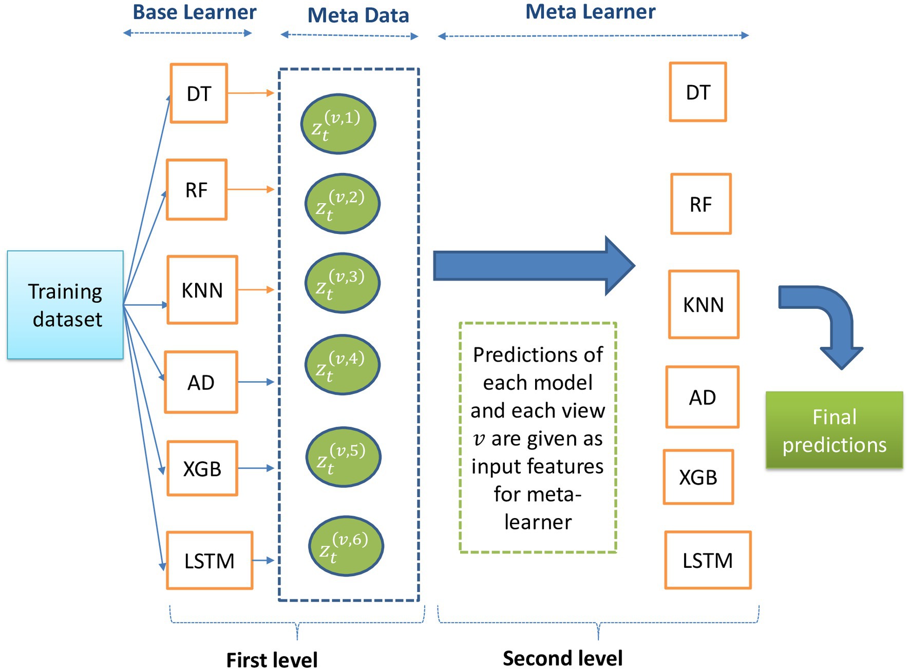
Multi-view stacking involves training multiple models (the “base learners”) on separate views of the data and fusing their outputs through stacked generalization. The predictions generated by the base learners serve as the training data for a final model called the meta-learner (Figure 4). This allows the meta-learner to identify patterns and relationships across the different views, leading to a more robust and accurate model. The overall procedure is outlined as follows:
1. Data preparation: Initialize with the time series views for time points , where each view contains distinct features across all time points. The outcomes are denoted by .
2. Training base learners: For each view from 1 to , iterate through base learners indexed by to , training each base learner using the view alongside the outcomes .
3. Time series validation and prediction generation:
- For each view and base learner , apply time series validation by partitioning the dataset chronologically into a series of training sets.
- Each base learner is trained on the respective training set and then makes predictions on the subsequent validating set, creating prediction vectors for each time point .
4. Constructing the meta-learner’s training set: Concatenate the prediction vectors from all base learners for each time point to form the matrix , which will serve as the training data for the meta-learner.
5. Meta-learner training: Use the combined predictions matrix and the true outcomes to train the meta-learner .
6. Final prediction model assembly: Utilize the meta-learner to integrate the base learners’ predictions, thus constructing the final multi-view stacking model that yields predictions for each time point.
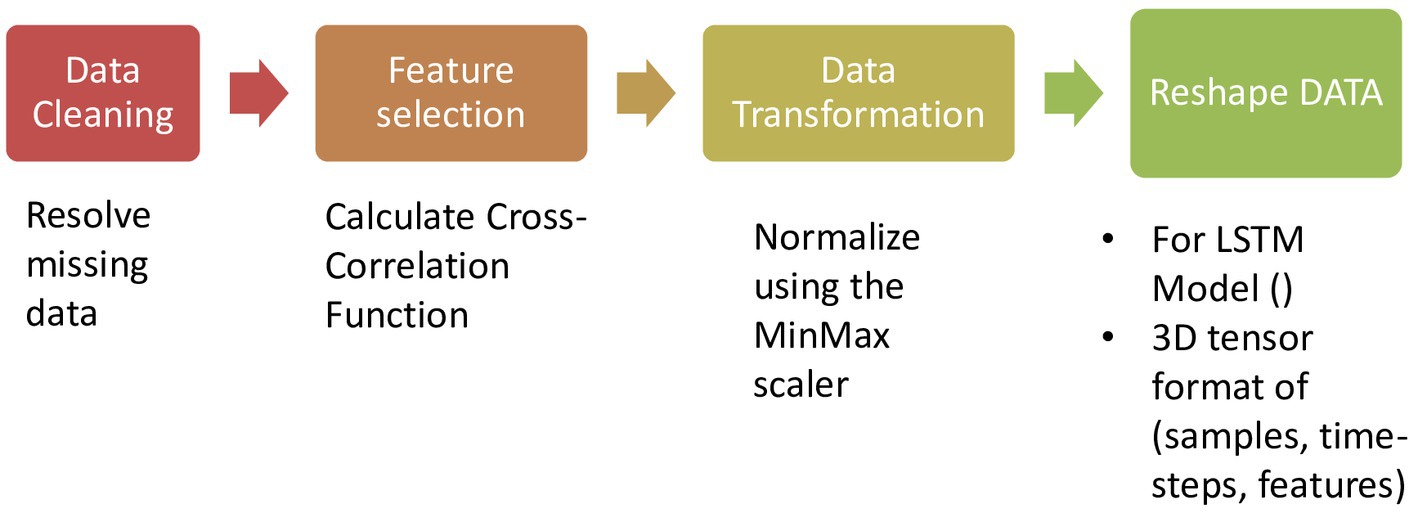
Figure 4. Description of multi-view learning approach steps to combine the predictions of multiple models.
The technique of time series cross-validation is used to prevent overfitting, ensuring that meta-models are not predicting on the same dataset they were trained with.
2.4 Walk-forward validation
Time series forecasting presents unique challenges compared to simpler problems like classification and regression. It involves the complexity of temporal dependency between observations, which requires specialized handling of data during model fitting and evaluation. However, this temporal structure also offers opportunities for improved modeling by capturing additional patterns such as trends and seasonality, leading to enhanced forecast accuracy.
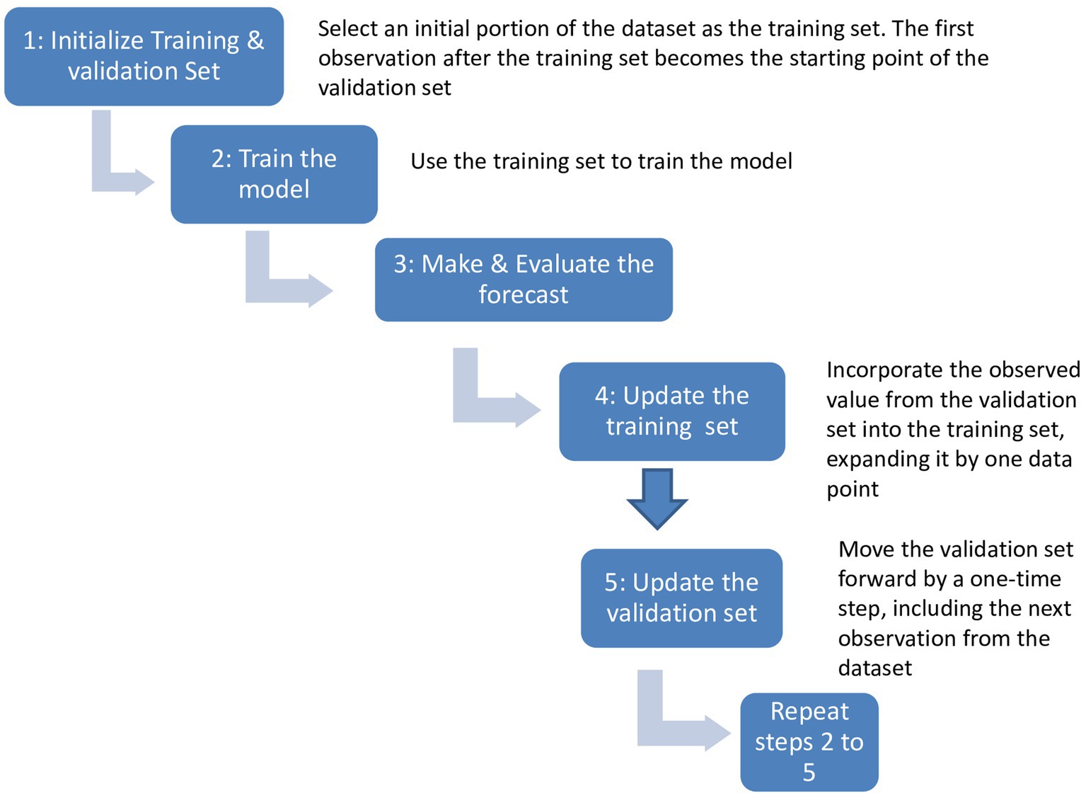
Conventional ML methods, such as train-test splits and k-fold cross-validation, are effective for other types of data but not for time series analysis because they do not take into account the time aspects of the data. To overcome this limitation, walk-forward validation is used. As presented in Figure 5, it consists of splitting the entire dataset into two parts: a training set and a validation set. The model is trained using the training set, and the forecasted values are then compared against the expected values using the validation set. At each time step, the forecasted value is incorporated into the training set, and this process is repeated iteratively. By continuously updating the model with newly forecasted values, the trained model can be effectively evaluated using walk-forward validation. This approach provides a realistic evaluation of time series data by incorporating the most up-to-date information available.
2.5 Hyperparameters optimization
The process of hyperparameter optimization, an important step in building a model, significantly impacts algorithmic performance. Hyperparameters define the model architecture and the complexity of each algorithm. Identifying their optimal values involves iterative experimentation with various combinations and assessing each model’s effectiveness. Poornima and Pushpalatha (2019) underscore the importance of searching for hyperparameters that boost its performance. A selective hyperparameter grid search, adapted for time series, was employed on the dataset, targeting the reduction of RMSE metrics.
Hyperparameters of tree-based models that conventionally need to be optimized include the maximum depth of the tree, the minimum number of samples, and the minimum number of samples required to create a leaf node. A tree that is too large results in a more complex model that can overfit the training data and consequently may not generalize well. In the case of RF, hyperparameter tuning includes the number of trees in the forest, the maximum depth of the trees, and the minimum number of samples required to split a node. The number of neighbors k is one of the principal hyperparameters of the KNN algorithm. It indicates the number of nearest neighbors used for forecasting. The larger k is, the more stable the model is. Conversely, smaller values of k suggest that the model is more sensitive to single points. Additionally, a weighting function is used to weigh the influence of each neighborhood on the prediction.
With regards to AdaBoost, some of the hyperparameters subject to optimization comprise the number of estimators and the learning rate. For XGBoost, the learning rate, max depth, and number of estimators are some hyperparameters to be tuned. A smaller learning rate requires more training iterations to reach a good model, but it can lead to higher accuracy. A larger number of trees can also make the model more computationally expensive to train and use.
In the implementation of LSTM models, the usual hyperparameter models are as follows:
• Learning rate: A small learning rate may slow convergence but may improve performance.
• Number of hidden units: A larger number of hidden units permits the model to learn more complex structures in the data but also increases the risk of overfitting.
• Number of layers: A deeper model can learn more complex patterns in the data but can also be computationally expensive and lead to overfitting.
• Dropout rate: Dropout is a regularization technique that prevents overfitting.
• Sequence Length: This is the number of time steps in each input sequence. Longer sequence lengths permit the model to capture long-term dependencies in the data but subject it to overfitting.
• Mini-batch size: Bigger mini-batch sizes accelerate training but make the model more prone to noise in the data.
• Number of epochs: Training for multiple epochs allows the model to continue to enhance, but it can also amplify the risk of overfitting if the model is already performing well on the training data.
2.6 Performance evaluation metrics
This section outlines the three commonly used statistical metrics for evaluating the performance of precipitation forecasting models:
1. Root mean squared error (RMSE).
2. Mean absolute error (MAE).
3. Coefficient of determination (R2).
RMSE evaluates the difference between observed and predicted values by squaring the errors, making it sensitive to large errors. MAE is less impacted by extreme values but can still be influenced by the size and number of observations. A low MAE value means that the model’s predictions are, on average, close to the actual values. R2, on the other hand, shows the extent to which the model can explain the variance and has a maximum score of 1.0, with a higher score indicating a better fit. The formulas for metrics are shown in Equations (3)–(5):
where , and design the predicted and observed monthly precipitation for test period t, respectively, i represents the month in the data set, and N is the length (total of test items in the data set) for the period t, is the mean values of the series .
3 Results
3.1 Prediction machine learning models results
Six prediction models, including five supervised learning algorithms (the DT, RF, KNN, AdaBoost, and XGBoost) and one deep learning algorithm (LSTM), were implemented in Python 3.10.9 using Keras 2.12.0. To identify the most relevant variables for model input, the cross-correlation function (CCF) was employed across lags ranging from 1 to 12 months. These include lagged values for precipitation, maximal and minimal temperatures, and insolation, which are pivotal in understanding the temporal dynamics influencing rainfall patterns, with the findings detailed in Table 2.
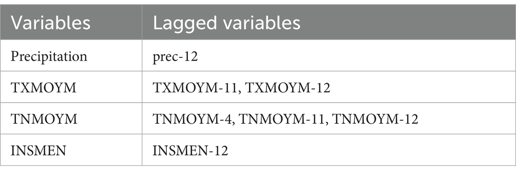
Table 2. The variables and their time lagged values used as input features for the selected models to predict monthly precipitation.
The selection of a 12-month lag for precipitation (prec-12) suggests that the models account for the influence of annual climatic cycles on rainfall, a factor especially critical in regions experiencing marked seasonal variations, where the amount of rainfall in a specific month may be affected by the weather patterns of the same month in the previous year. Similarly, the incorporation of lagged temperatures (TXMOYM-11, TXMOYM-12 for maximum and TNMOYM-4, TNMOYM-11, TNMOYM-12 for minimum temperatures) reflects the model’s consideration of both short-term and long-term temperatures in predicting current precipitation. This indicates the cyclical or delayed impact of temperature on present climatic conditions through factors like evaporation rates and soil moisture. Additionally, the integration of a 12-month lag for insolation (INSMEN-12) underscores its role in current precipitation predictions. This could be due to the influence of insolation on the process of evaporation and the patterns of atmospheric circulation, which are key factors in rainfall creation.
Consequently, the variables TXMOYM, TNMOYM, and INSMEN, enriched by the lagged variables identified through CCF, form the inputs of our predictive models. The models are built to capture both short-term fluctuations and long-term trends in climatic conditions, enhancing their predictive capability in a region characterized by its Mediterranean climate and distinct seasonal and annual climatic cycles, such as Rabat, Morocco.
To identify the most optimal configuration for each model, a hyperparameter search was performed on multiple machine learning models. The hyperparameter evaluations are presented in Table 3, which details the optimal hyperparameters and their corresponding value ranges utilized in the fine-tuning process. The performance metrics for the training and test sets are displayed in Table 4. AdaBoost, RF, and XGBoost demonstrated good performance on the training set, achieving RMSEs of 28.3, 30.5, and 34.7, respectively. XGBoost outperforms other models on the test set with an RMSE of 40.8, implying superior generalization. The significant performance gap between training and test sets for all models suggests the presence of overfitting. To address this issue, multi-view stacking learning is proposed as a potential solution to capture the intricate temporal pattern of monthly rainfall with enhanced accuracy and reliability.
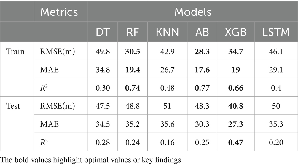
Table 4. Performance metrics (RMSE, MAE, R2) for individual prediction models (DT, RF, KNN, AB, XGB, LSTM).
3.2 Multi-view stacking learning results
As mentioned in Section 2, multi-view stacking learning is an ensemble learning technique where multiple models are trained for each feature separately to make first-level predictions. These predictions are then aggregated and serve as inputs for the meta-model, which produces the final prediction. At the first level, a variety of models, including Decision Tree (DT), Random Forest (RF), K-Nearest Neighbors (KNN), AdaBoost, XGBoost, and Long Short-Term Memory (LSTM) are trained on the selected input variables, as detailed in Table 2. At the second level, the same models involved in the first level are trained using the constructed meta-base. This meta-base can be created in two distinct ways: either by employing the same base learner across all views or by integrating a diverse set of base learners assigning a unique one for each view. The performance outcomes from this training process are displayed in Tables 5, 6.
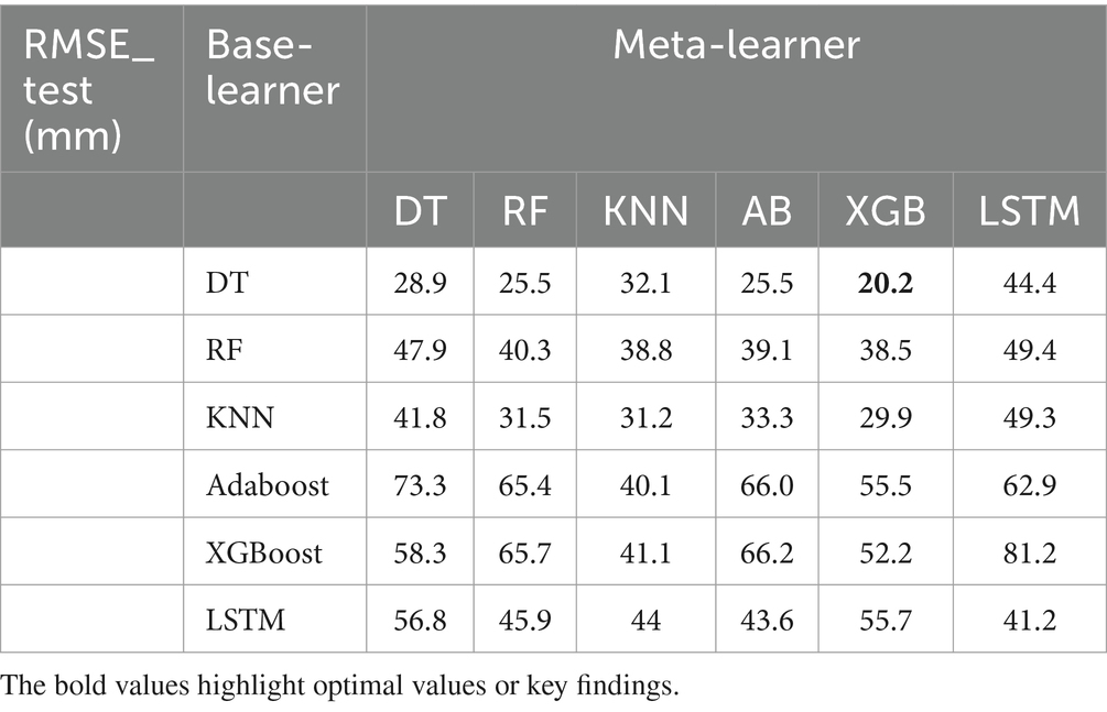
Table 5. Comparative RMSE_test(mm) values for different combinations of base learners (DT, RF, KNN, AB, XGB, and LSTM) and meta-learners (DT, RF, KNN, AB, XGB, and LSTM).
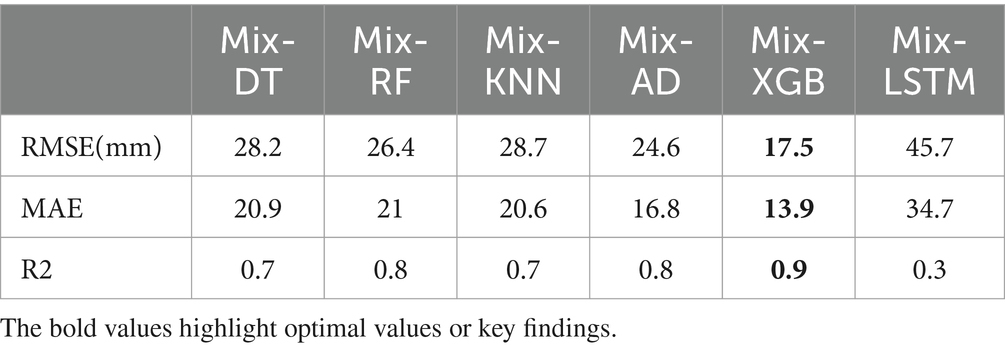
Table 6. Performance metrics for mixed-base learners for each meta-learner (DT, RF, KNN, AB, XGB, LSTM).
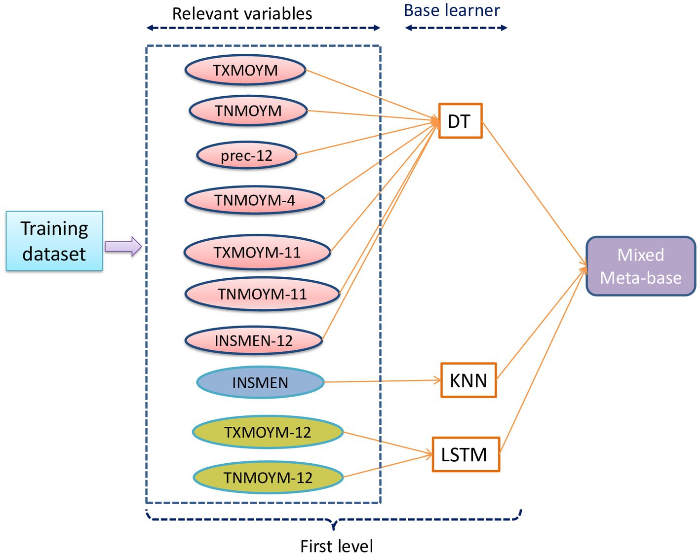
The evaluation metrics for the first approach are presented in Table 5. It revealed that the DT, as a base learner, shows promising results, achieving RMSEs that range from 20.2 mm to 44.4 mm. Notably, the integration of XGBoost as a meta-learner consistently amplifies the performance of DT, underscoring the robustness and effectiveness of XGBoost in synthesizing insights from the base learners. RF performs optimally when combined with XGBoost, KNN, AdaBoost, or itself, yielding corresponding RMSEs of 38.5 mm, 38.8 mm, and 39.1 mm. KNN achieves good results when combined with XGBoost, itself, RF, and AdaBoost, with corresponding RMSEs of 29.9 mm, 31.2 mm, 31.5 mm, and 33.3 mm, respectively. Both AdaBoost and XGBoost achieve optimal performance when paired with KNN, achieving respective RMSEs of 40.1 mm and 41.1 mm. However, they underperform when combined with other models. When LSTM is used with itself, AdaBoost, KNN, and Random Forest, it achieves its best level of performance, with respective RMSEs of 29.9 mm, 31.2 mm, 31.5 mm, and 33.3 mm. Overall, DT stands out as the top-performing base learner in terms of overall performance, followed by KNN. Conversely, RF, AdaBoost, XGBoost, and LSTM exhibit comparatively lower performance compared to other base learners. Among the meta-learners, XGBoost emerged as the most efficient meta-learner. The outcomes presented in Table 6 show that the second approach yields the optimal performance (Figure 6). A mixed-base learner, created using the combinations illustrated in Figure 7, coupled with the meta-learner XGBoost (Mix-XGB), achieves the best RMSE of 17.5 mm. Boxplots, scatterplots, violin plots, and Taylor diagrams further solidify these results. The boxplot graph (Figure 8A) confirms XGBoost’s superior alignment with the observed distribution. Conversely, the wider distributions of DT, Adaboost, and LSTM suggest greater variability in their predictions. Scatterplots (Figure 8B) reveal that while most models follow the overall pattern, there are deviations, especially at higher precipitation levels. This suggests that most models perform well for low to moderate rainfall predictions but struggle with significant rainfall events. The Taylor diagram (Figure 9A) reinforces these observations. The models are clustered in the areas exhibiting high correlation coefficients. However, the spread of these models suggests divergent degrees of accuracy, as indicated by their varying distances from the reference point. Notably, the Mix-XGB model stands out, reflecting a high correlation and a smaller centered RMS difference when compared to models like Mix-LSTM. Violin plots (Figure 9B) offer another perspective. Although Mix-RF displays a wider spread, suggesting its ability to capture a wide range of precipitation, including extremes, Mix-XGB’s distribution maintains a balance between encompassing variability and maintaining a concentrated focus around the average real precipitation.

Figure 6. Graph of observed and predicted precipitations: Models with mixed-base learners and (RF, DT, KNN, AdaBoost, XGBoost) as meta-learners.
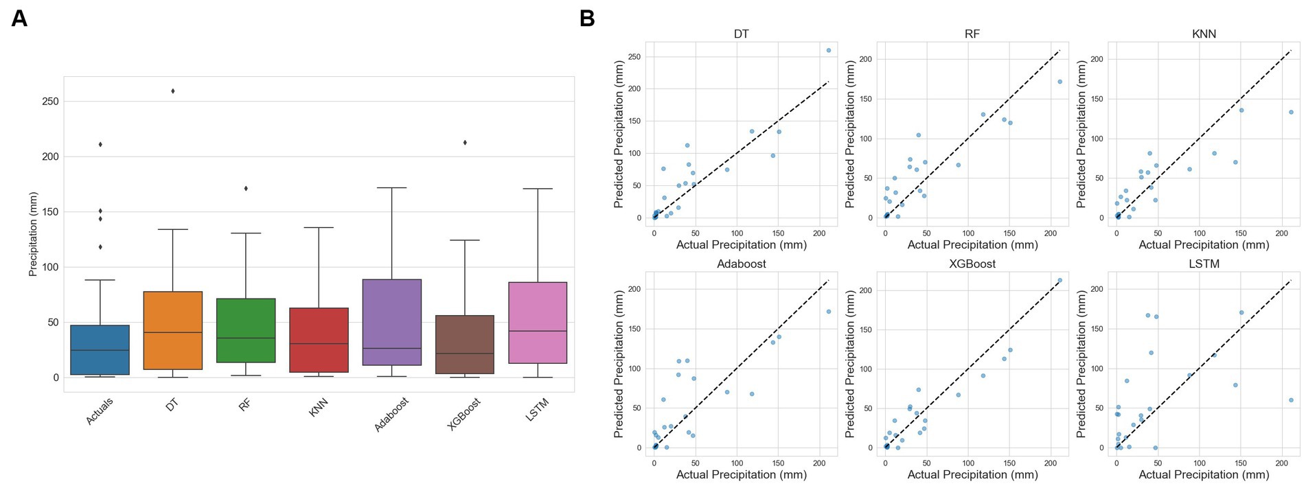
Figure 8. (A) Box Plot (B) Scatter Plot for DT, RF, KNN, Adaboost, Xgboost, and LSTM models using multi-view stacking learning approach based on mixed-base learners.
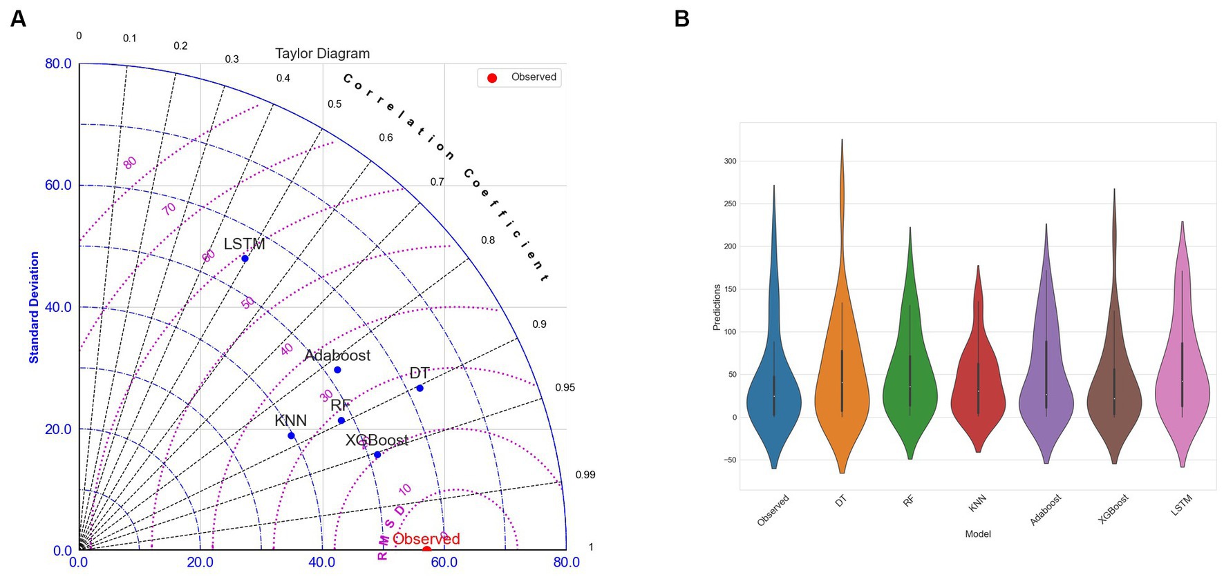
Figure 9. (A) Taylor Diagram (B) Violin Plot for DT, RF, KNN, Adaboost, Xgboost, and LSTM models using multi-view stacking learning approach based on mixed-base learners.
The findings of this study demonstrate the potential of multi-view stacking learning. By combining different perspectives on the data (multi-view) and leveraging the strengths of multiple models (stacking) at two levels, this approach significantly improves the accuracy of rainfall predictions, setting the stage for a deeper understanding of complex fields like climate data analysis.
4 Discussion
The results evoke the complex relationship between meteorological factors and intensities, a dynamic increasingly affected by climate change. These trends are driven by a mixture of distinct local weather conditions, such as temperature and sunshine, which are also influenced by changes in global climate dynamics. The superior performance of multi-view stacking learning techniques, particularly the combination of Decision Tree, LSTM, and XGBoost, can be explained by the complementary nature of these algorithms. As mentioned by Bamisile et al. (2022), each algorithm has different strengths. While decision trees provide understandable models and handle nonlinear data efficiently, LSTM captures sequential dependencies and recognizes time-dependent structures, and XGBoost incentivizes weak learners to develop a robust model. Their combination effectively captures both temporal patterns and nonlinear relationships with covariates. The results highlight the importance of preserving and combining algorithm performance across different dimensions of the dataset. Ignoring these unique perspectives could result in the loss of crucial information that can guide the model toward more accurate predictions. This technique contrasts with traditional methods, which may not account for the multidimensional nature of climate data, often leading to overfitting and poor generalization. The proposed multi-view stacking technique effectively addresses this challenge, particularly for the examined study, which is characterized by stays that will mainly take place from November to March with strong spatial and temporal variability.
Numerous studies have explored the prediction of monthly precipitation patterns, such as those conducted by Tharun et al. (2018), Chhetri et al. (2020), Chen et al. (2022), Gu et al. (2022) and Zandi et al., (2022). Typically, their focus was on using single-model approaches or ensemble methods. While these strategies can be effective in specific scenarios, they may encounter difficulties with the complex, multidimensional nature of climate data. The present study investigates the application of a multi-view learning strategy, which has not been thoroughly studied. A key aspect of the present work is the incorporation of lagged variables, which are essential in capturing the delayed effects of climatic factors on rainfall and predicting the intricate temporal dynamics inherent in meteorological data. This research is distinctive in its use of multiple base learners, including the LSTM network. The integration of meta-learners, particularly XGBoost and AdaBoost, to incorporate information from diverse sources further enriches the research. This work is among the few that centers its focus on Morocco, offering specific insights for the region and underscoring the potential impacts of climate change on localized precipitation patterns, which are essential for the development of local strategies.
5 Conclusion
This study investigated the application of machine learning models to monthly rainfall data in Rabat, Morocco, aiming to enhance forecast accuracy using a multi-view stacking learning technique. Historical weather data from Rabat was employed to assess the effectiveness of the forecast models. The evaluation process included multiple important steps: data preprocessing to handle missing values and normalize the data, selection of the most relevant variables using the cross-correlation function (CCF) to analyze lag effects, and hyperparameter grid search to optimize model performance. Five ML algorithms (DT, RF, KNN, AdaBoost, and XGBoost), as well as an LSTM network, were tested.
The optimal performance resulted from integrating the relevant variables (prec-12, TXMOYM, TXMOYM-11, TXMOYM-12, TNMOYM, TNMOYM-4, TNMOYM-11, TNMOYM-12, INSMEN, INSMEN-12) within a mixed meta-base that leveraged a combination of base learners (DT, KNN, LSTM). These results emphasized the critical importance of choosing appropriate core learners and combining relevant variables. The study also underscores the promising potential of XGBoost and AdaBoost as meta-learners to integrate and leverage information from multiple sources, resulting in predictive performance enhancement.
While multi-view stacking learning techniques have enhanced prediction accuracy, they have also introduced complexity into the model development and training processes. This complexity can increase the risk of overfitting. Despite employing techniques like cross-validation adapted for time series to mitigate this risk, achieving a balance between model complexity and generalization remains a challenging aspect that must be carefully managed. Furthermore, the capacity to generalize and adapt these models to other geographical regions and climatic types is still a potential area requiring further investigation, especially given the limitations of the dataset size used for training these models. More investigation is needed to examine the model’s effectiveness using larger and more diverse sources of datasets to improve its potential to generalize and capture future climate variability, particularly as climate change accelerates.
Focusing on the specific context of Morocco—a region that frequently experiences strong El Niño-Southern Oscillation (ENSO) events and, less frequently, La Niña episodes—underscores the complexity of its climate. This complexity, coupled with the critical need for precise precipitation forecasts, suggests that the Moroccan climate requires more in-depth investigation. The proposed approaches could be considered on a broader spatial scale beyond the scope of the present study. Further investigation of several Moroccan stations with varying meteorological characteristics and additional relevant factors would improve our understanding of the variability of precipitation patterns and climate change in the country. Additionally, further exploration of other promising ML models and techniques, including transformers, is crucial for a comprehensive understanding of regional precipitation patterns and the impacts of climate change.
Data availability statement
The datasets used in this study are not publicly available since they are the property of the Directorate of Meteorology in Morocco, but they may be made available upon reasonable request from the corresponding author.
Author contributions
MH: Conceptualization, Data curation, Formal analysis, Investigation, Methodology, Software, Validation, Writing – original draft, Writing – review & editing. KH: Investigation, Methodology, Supervision, Validation, Writing – review & editing. S-EA: Investigation, Visualization, Writing – review & editing.
Funding
The author(s) declare that no financial support was received for the research, authorship, and/or publication of this article.
Conflict of interest
The authors declare that the research was conducted in the absence of any commercial or financial relationships that could be construed as a potential conflict of interest.
Publisher’s note
All claims expressed in this article are solely those of the authors and do not necessarily represent those of their affiliated organizations, or those of the publisher, the editors and the reviewers. Any product that may be evaluated in this article, or claim that may be made by its manufacturer, is not guaranteed or endorsed by the publisher.
References
Abhishek, K., Kumar, A., Ranjan, R., and Kumar, S. (2012). “A rainfall prediction model using artificial neural network” in 2012 IEEE Control and System Graduate Research Colloquium (IEEE), 82–87. doi: 10.1109/ICSGRC.2012.6287140
Ahsan, S., Bhat, M. S., Alam, A., Farooq, H., and Shiekh, H. A. (2022). Evaluating the impact of climate change on extreme temperature and precipitation events over the Kashmir Himalaya. Clim. Dyn. 58, 1651–1669. doi: 10.1007/s00382-021-05984-6
Balan, M. S., Selvan, J. P., Bisht, H. R., Gadgil, Y. A., Khaladkar, I. R., and Lomte, V. M. (2019). Rainfall prediction using deep learning on highly non-linear data. Int. J. Res. Eng. Sci. Manage. 2, 590–592
Bamisile, O., Ejiyi, C. J., Osei-Mensah, E., Chikwendu, I. A., Li, J., and Huang, Q. (2022). “Long-term prediction of solar radiation using XGboost, LSTM, and machine learning algorithms” in 2022 4th Asia Energy and Electrical Engineering Symposium (AEEES) (IEEE), 214–218. doi: 10.1109/AEEES54426.2022.9759719
Baudhanwala, D., Mehta, D., and Kumar, V. (2024). Machine learning approaches for improving precipitation forecasting in the Ambica River basin of Navsari District, Gujarat. Water Pract. Technol. 19, 1315–1329. doi: 10.2166/wpt.2024.079
Blum, A., and Mitchell, T. (1998). “Combining labeled and unlabeled data with co-training” in Proceedings of the Eleventh Annual Conference on Computational Learning Theory, 92–100. doi: 10.1145/279943.279962
Bojang, P. O., Yang, T.-C., Pham, Q. B., and Yu, P.-S. (2020). Linking singular spectrum analysis and machine learning for monthly rainfall forecasting. Appl. Sci. 10:3224. doi: 10.3390/app10093224
Brahim, Y. A., Bouchaou, L., Sifeddine, A., Khodri, M., Reichert, B., and Cruz, F. W. (2016). Elucidating the climate and topographic controls on stable isotope composition of meteoric waters in Morocco, using station-based and spatially-interpolated data. J. Hydrol. 543, 305–315. doi: 10.1016/j.jhydrol.2016.10.001
Chen, T., and Guestrin, C. (2016). “Xgboost: a scalable tree boosting system” in Proceedings of the 22nd ACM SIGKDD International Conference on Knowledge Discovery and Data Mining, 785–794. doi: 10.1145/2939672.2939785
Chen, C., Zhang, Q., Kashani, M. H., Jun, C., Bateni, S. M., Band, S. S., et al. (2022). Forecast of rainfall distribution based on fixed sliding window long short-term memory. Eng. Appl. Comput. Fluid Mech. 16, 248–261. doi: 10.1080/19942060.2021.2009374
Chhetri, M., Kumar, S., Pratim Roy, P., and Kim, B.-G. (2020). Deep BLSTM-GRU model for monthly rainfall prediction: a case study of Simtokha, Bhutan. Remote Sens. 12:3174. doi: 10.3390/rs12193174
Danandeh Mehr, A., Nourani, V., Karimi Khosrowshahi, V., and Ghorbani, M. A. (2019). A hybrid support vector regression–firefly model for monthly rainfall forecasting. Int. J. Environ. Sci. Technol. 16, 335–346. doi: 10.1007/s13762-018-1674-2
Dash, Y., Mishra, S. K., and Panigrahi, B. K. (2018). Rainfall prediction for the Kerala state of India using artificial intelligence approaches. Comput. Electr. Eng. 70, 66–73. doi: 10.1016/j.compeleceng.2018.06.004
Driouech, F., Stafi, H., Khouakhi, A., Moutia, S., Badi, W., ElRhaz, K., et al. (2021). Recent observed country-wide climate trends in Morocco. Int. J. Climatol. 41, E855–E874. doi: 10.1002/joc.6734
El Hafyani, M., and El Himdi, K. (2022). “A comparative study of geometric and exponential Laws in modelling the distribution of daily precipitation durations” in IOP Conference Series: Earth and Environmental Science (IOP Publishing). doi: 10.1088/1755-1315/1006/1/012005
Esposito, F., Malerba, D., Semeraro, G., and Kay, J. (1997). A comparative analysis of methods for pruning decision trees. IEEE Trans. Pattern Anal. Mach. Intell. 19, 476–493. doi: 10.1109/34.589207
Freund, Y., and Schapire, R. E. (1997). A decision-theoretic generalization of on-line learning and an application to boosting. J. Comput. Syst. Sci. 55, 119–139. doi: 10.1006/jcss.1997.1504
Garcia-Ceja, E., Galván-Tejada, C. E., and Brena, R. (2018). Multi-view stacking for activity recognition with sound and accelerometer data. Inform Fusion 40, 45–56. doi: 10.1016/j.inffus.2017.06.004
Garg, A., and Pandey, H. (2019). Rainfall prediction using machine learning. Int. J. Innov. Sci. Res. Technol. 4, 56–58. doi: 10.13140/RG.2.2.26691.04648
Gnanasankaran, N., and Ramaraj, E. (2020). A multiple linear regression model to predict rainfall using Indian meteorological data. Int. J. Adv. Sci. Technol. 29, 746–758
Gohil, M., Mehta, D., and Shaikh, M. (2024). An integration of geospatial and fuzzy-logic techniques for multi-hazard mapping. Resul. Eng. 21:101758. doi: 10.1016/j.rineng.2024.101758
Gu, J., Liu, S., Zhou, Z., Chalov, S. R., and Zhuang, Q. (2022). A stacking ensemble learning model for monthly rainfall prediction in the Taihu Basin, China. Water 14:492. doi: 10.3390/w14030492
Hochreiter, S., and Schmidhuber, J. (1997). Long short-term memory. Neural Comput. 9, 1735–1780. doi: 10.1162/neco.1997.9.8.1735
Hung, N. Q., Babel, M. S., Weesakul, S., and Tripathi, N. K. (2009). An artificial neural network model for rainfall forecasting in Bangkok, Thailand. Hydrol. Earth Syst. Sci. 13, 1413–1425. doi: 10.5194/hess-13-1413-2009
Huntingford, C., Jeffers, E. S., Bonsall, M. B., Christensen, H. M., Lees, T., and Yang, H. (2019). Machine learning and artificial intelligence to aid climate change research and preparedness. Environ. Res. Lett. 14:124007. doi: 10.1088/1748-9326/ab4e55
Javan, K., and Movaghari, A. R. (2022). Assessment of climate change impacts on extreme precipitation events in Lake Urmia Basin, Iran. Desert 27, 13–33. doi: 10.22059/JDESERT.2022.88507
Krysanova, V., Vetter, T., Eisner, S., Huang, S., Pechlivanidis, I., Strauch, M., et al. (2017). Intercomparison of regional-scale hydrological models and climate change impacts projected for 12 large river basins worldwide—a synthesis. Environ. Res. Lett. 12:105002. doi: 10.1088/1748-9326/aa8359
Kumar, V., Kedam, N., Sharma, K. V., Mehta, D. J., and Caloiero, T. (2023). Advanced machine learning techniques to improve hydrological prediction: a comparative analysis of streamflow prediction models. Water 15:2572. doi: 10.3390/w15142572
Kumar, D., Singh, A., Samui, P., and Jha, R. K. (2019). Forecasting monthly precipitation using sequential modelling. Hydrol. Sci. J. 64, 690–700. doi: 10.1080/02626667.2019.1595624
Liu, J., Long, A., Deng, X., Yin, Z., Deng, M., An, Q., et al. (2022). The impact of climate change on hydrological processes of the Glacierized watershed and projections. Remote Sens. 14:1314. doi: 10.3390/rs14061314
Mehta, D., Dhabuwala, J., Yadav, S. M., Kumar, V., and Azamathulla, H. M. (2023). Improving flood forecasting in Narmada river basin using hierarchical clustering and hydrological modelling. Resul. Eng. 20:101571. doi: 10.1016/j.rineng.2023.101571
Näschen, K., Diekkrüger, B., Leemhuis, C., Seregina, L. S., and van der Linden, R. (2019). Impact of climate change on water resources in the Kilombero catchment in Tanzania. Water 11:859. doi: 10.3390/w11040859
Parmesan, C., Morecroft, M. D., and Trisurat, Y. (2022). Climate change 2022: impacts, adaptation, and vulnerability. GIEC.
Patel, A., Vyas, D., Chaudhari, N., Patel, R., Patel, K., and Mehta, D. (2024). Novel approach for the LULC change detection using GIS & Google Earth Engine through spatiotemporal analysis to evaluate the urbanization growth of Ahmedabad city. Resul. Eng. 21:101788. doi: 10.1016/j.rineng.2024.101788
Poornima, S., and Pushpalatha, M. (2019). Prediction of rainfall using intensified LSTM-based recurrent neural network with weighted linear units. Atmos 10:668. doi: 10.3390/atmos10110668
Singh, P., and Borah, B. (2013). Indian summer monsoon rainfall prediction using artificial neural network. Stoch. Env. Res. Risk A. 27, 1585–1599. doi: 10.1007/s00477-013-0695-0
Tharun, V. P., Prakash, R., and Devi, S. R. (2018). “Prediction of rainfall using data mining techniques” in 2018 Second International Conference on Inventive Communication and Computational Technologies (ICICCT) (IEEE), 1507–1512. doi: 10.1109/ICICCT.2018.8473177
Tramblay, Y., Villarini, G., El Khalki, E. M., Gründemann, G., and Hughes, D. (2021). Evaluation of the drivers responsible for flooding in Africa. Water Resour. Res. 57:e2021WR029595. doi: 10.1029/2021WR029595
Trenberth, K. E. (2011). Changes in precipitation with climate change. Clim. Res. 47, 123–138. doi: 10.3354/cr00953
van Loon, W., Fokkema, M., Szabo, B., and de Rooij, M. (2020). Stacked penalized logistic regression for selecting views in multi-view learning. Inform. Fusion 61, 113–123. doi: 10.1016/j.inffus.2020.03.007
Verma, S., Verma, M. K., Prasad, A. D., Mehta, D., Azamathulla, H. M., Muttil, N., et al. (2023). Simulating the hydrological processes under multiple land use/land cover and climate change scenarios in the mahanadi reservoir complex, Chhattisgarh, India. Water 15:3068. doi: 10.3390/w15173068
Wang, C., Jia, Z., Yin, Z., Liu, F., Lu, G., and Zheng, J. (2021). Improving the accuracy of subseasonal forecasting of China precipitation with a machine learning approach. Front. Earth Sci. 9:659310. doi: 10.3389/feart.2021.659310
Wolpert, D. H. (1992). Stacked generalization. Neural Netw. 5, 241–259. doi: 10.1016/S0893-6080(05)80023-1
Wunsch, A., Liesch, T., and Broda, S. (2022). Deep learning shows declining groundwater levels in Germany until 2100 due to climate change. Nat. Commun. 13:1221. doi: 10.1038/s41467-022-28770-2
Zandi, O., Zahraie, B., Nasseri, M., and Behrangi, A. (2022). Stacking machine learning models versus a locally weighted linear model to generate high-resolution monthly precipitation over a topographically complex area. Atmos. Res. 272:106159. doi: 10.1016/j.atmosres.2022.106159
Zhang, Z. (2016). Introduction to machine learning: k-nearest neighbors. Ann. Transl. Med 4:218. doi: 10.21037/atm.2016.03.37
Zhang, H., Zhang, L. L., Li, J., An, R. D., and Deng, Y. (2018). Climate and hydrological change characteristics and applicability of GLDAS data in the Yarlung Zangbo River basin, China. Water 10:254. doi: 10.3390/w10030254
Keywords: rainfall prediction, machine learning, multi-view learning, stacking learning, multivariate time series, Morocco, North Africa
Citation: El Hafyani M, El Himdi K and El Adlouni SE (2024) Improving monthly precipitation prediction accuracy using machine learning models: a multi-view stacking learning technique. Front. Water. 6:1378598. doi: 10.3389/frwa.2024.1378598
Edited by:
Evangelos Rozos, Institute for Environmental Research and Sustainable Development, GreeceReviewed by:
Wen-Ping Tsai, National Cheng Kung University, TaiwanJamshid Piri, Zabol University, Iran
Copyright © 2024 El Hafyani, El Himdi and El Adlouni. This is an open-access article distributed under the terms of the Creative Commons Attribution License (CC BY). The use, distribution or reproduction in other forums is permitted, provided the original author(s) and the copyright owner(s) are credited and that the original publication in this journal is cited, in accordance with accepted academic practice. No use, distribution or reproduction is permitted which does not comply with these terms.
*Correspondence: Mounia El Hafyani, bW91bmlhX2VsaGFmeWFuaUB1bTUuYWMubWE=
 Mounia El Hafyani
 Khalid El Himdi
 Salah-Eddine El Adlouni

