An active learning convolutional neural network for predicting river flow in a human impacted system

The South Platte river system contains a mixture of natural streams, reservoirs, and pipeline projects that redirect water to front range communities in Colorado. At many timepoints, a simple persistence model is the best predictor for flow from pipelines and reservoirs but at other times, flows change based on snowmelt and inputs such as reservoir fill rates, local weather, and anticipated demand. Here we find that a convolutional Long Short-Term Memory (LSTM) network is well suited to modeling flow in parts of this basin that are strongly impacted by water projects as well as ones that are relatively free from direct human modifications. Furthermore, it is found that including an active learning component in which separate Convolutional Neural Networks (CNNs) are used to classify and then select the data that is then used for training a convolutional LSTM network is advantageous. Models specific for each gauge are created by transfer of parameter from a base model and these gauge-specific models are then fine-tuned based a curated subset of training data. The result is accurate predictions for both natural flow and human influenced flow using only past river flow, reservoir capacity, and historical temperature data. In 14 of the 16 gauges modeled, the error in the prediction is reduced when using the combination of on-the-fly classification by CNN followed by analysis by either a persistence or convolutional LSTM model. The methods designed here could be applied broadly to other basins and to other situations where multiple models are needed to fit data at different times and locations.

1. Introduction

Machine learning methods for numerical prediction of streamflow have recently been utilized alongside traditional hydrological models. CNNs have been used to predict flow in rivers (Duan et al., 2020; Shu et al., 2021) and in urban areas prone to flooding (Chiacchiera et al., 2022). Recurrent Neural Networks (RNNs) have also been used to predict flow (van der Lugt and Feelders, 2020). These and other deep learning methods have been recently reviewed (Sit et al., 2020; Le et al., 2021) including the role of deep learning methods in predicting flow in urban areas (Fu et al., 2022). LSTM models are particularly well-suited to time-series forecasting (Sagheer and Kotb, 2019) as they retain time-dependent connections and a number of studies have shown that LSTM models incorporating hydrological inputs can successfully predict rainfall runoff (Kratzert et al., 2018; Poornima and Pushpalatha, 2019; Xiang et al., 2020) over both short and medium timescale (Granata and Di Nunno, 2023). However, the consensus is that innovation in deep learning models will be required to further improve forecasting over numerical models (Schultz et al., 2021).

The convolutional LSTM (Shi et al., 2015) is based on a fully connected LSTM but uses convolution outputs directly as part of reading input into the LSTM units. This approach is appealing to weather forecasting as it enables the patterns identified within past data, to be identified across time points in past data and projected forward in future predictions. Convolutional LSTMs have been used in applications as varied as predicting stock prices (Fang et al., 2021) and air cargo transport patterns (Anguita and Olariaga, 2023) and have recently been used for rainfall nowcasting (Liu et al., 2022) and flood forecasting (Moishin et al., 2021).

Here a river system that has a complicated combination of features many of which are highly impacted by human influence is modeled using both a CNN and a convolutional LSTM. Transfer learning, which has been successfully applied to benchmarked time series forecasting improving accuracy (Gikunda and Jouandeau, 2021), is used here to create gauge specific models after initial training on all gauges with a single model. This is combined with an active learning (Ren et al., 2021) approach to efficiently utilize the data available for training. Specifically, a CNN based classifier is used to select a subset of data most suitable for training the convolutional LSTM models and individual models for each predicted gauge are created through transfer learning from the base model. This same classification model is used to determine if a given set of input data is better modeled by a persistence model or the Convolutional LSTM for that gauge to provide on-the-fly model selection. This work uses a novel combination of transfer learning and active learning to account for the variability between the different streamflows being predicted. This combination improves the prediction accuracy of both the highly variable snowmelt driven gauges and the flows from water projects that have less variability over time. This method of combining classification and active learning approaches could be extended to combine other types of models.

2. Materials and methods

2.1. Model

The upper region of the South Platte river basin (Figure 1) serves as a water source for numerous communities. Colorado front range communities draw water from the South Platte and other nearby rivers to meet their water needs throughout the year. Data inputs were used from the major reservoirs (Stronita Springs, Cheesman, and Chatfield) along the South Platte, tunnels including ones that bring water across the Continental Divide (Roberts and Moffat tunnels) or move water within the drainage (homestake), and gauges representative of the many un-dammed streams (south fork of the South Platte, middle fork of Prince, and South Platte above Spinney), as well as gauges that are located below reservoirs (Eleven mile outflow, Antero outflow, below Brush creek, and Deckers), and the pipes (conduit 20 and 26) that send water from the reservoirs into Denver. Gauges were also included in the model that are outside of the South Platte drainage but are a part of the Denver Water system including South Boulder creek which supplies water to Denver and the Blue River below Dillon Reservoir which reflects releases of water into the Colorado that are therefore unavailable for transfer to the front range. Finally, gauges were included that do not directly supply water to the front range but that are connected indirectly because they are managed by Denver Water and governed by the Colorado River Compact of 1922 (MacDonnell, 2023) which sets the total amount of water that must be sent to downstream states. Transfers of water eastward across the Divide are often offset by releases into the Colorado River to comply with this compact.

FIGURE 1

Figure 1. Map showing region including location of the gauges examined in this study.

Gauges were selected for the final model by examining which gauges in this region showed strong correlations to each other within this river basin (Figure 2). Some strong correlations are due to close geography. For example, the majority of the flow out of Strontia Spring reservoir flows directly into Chatfield reservoir and these gauges have a 0.969203 Pearson correlation coefficient. In contrast, a correlation of −0.126896 is seen between the Roberts tunnel which brings water from Dillon reservoir across the continental divide to be used in Denver and the inflow to Cheesman reservoir, which feeds Denver from other sources east of the divide. When water is available east of the divide, water is not transported from west of the divide.

FIGURE 2

Figure 2. Correlation heatmap for raw data from all riverflow gauges using data from 1996 through 2021.

The homestake pipeline stands out as being negatively correlated with many of the other gauges. This project takes water from the South Platte basin and delivers it further south, to the city of Colorado Springs. Similarly, two other gauges that were geographically within this region but delivered water to the town of Aurora likewise had weaker correlations.

2.2. Data inputs

Data from 1996 through 2021 was collected using the Colorado Division of Water Resources (https://dwr.state.co.us/Rest/) Application Programming Interface. Outlier datapoints 2 times above the 95th percentile or below the 10th percentile in flow or capacity were removed. Historical weather data was obtained from the National Centers for Environmental Information (https://www.ncdc.noaa.gov/cdo-web/datasets) for the city of Lakewood, Colorado which is close to the region of study, receives water from this river system, and has a long and continuous set of temperature readings through the period of study. Training was performed on all days available where 21 prior days are included in the model and 7 future days are predicted.

2.3. Seasonality adjustments

While any river flow data is likely to have seasonal variation, the data used here presents unique challenges. In a river system heavily influenced by anthropogenic activity, not all gauges follow a similar pattern of seasonality. Some gauges on unmodified streams have seasonality expected for natural rivers with increased flow during spring snowmelt. Other gauges are inactive for long periods of time, and some have absolutely no variability for the majority of the year. Some of the gauges that are largely inactive become active during spring runoff, but others are countercyclical, changing little during the spring, but becoming more active at other times of year. For example, several tunnels bring water across the continental divide and are often most active in the fall when water demands in the front range cannot be met with natural flow from streams into reservoirs.

Winter data was removed because flow is negligible at most of the gauges, however, this creates a discontinuity in the data. While careful selection of start and end dates can avoid using data that crosses this discontinuity, it is desirable to have flexibility in data handling and training of the neural network. Ideal flexibility would allow for selecting gauges, past and future window lengths, and setting weights prior to editing out data that contains such discontinuities. Under these circumstances, a final step must be performed to remove data that crosses the discontinuity. Since there are no column labels on data used for training and validation, another method is needed for identifying data that crosses this discontinuity. For this reason, a unique identifier is created by multiplying two arbitrarily selected column values. This product acts as a unique identifier of discontinuities and it is used to identify datasets containing discontinuities to be removed immediately before training.

After combining all seasons, the data was split into three sets. The first set was used for training the neural networks. A second validation set used to periodically check the network against data that had not yet been seen by the model to protect against overfitting; when validation data did not improve the fit, fitting was stopped regardless of whether the training data was still improving the quality of fit. Finally, a third set of data was set aside and not used for training or validation but rather for testing the model. All evaluation reported here is based on how well the model handled this testing data that was not used for training or for validation. All the data was Z-score normalized and the mean and standard deviation for the training set was used to normalize the training, validation, and testing data sets to avoid risk of information creeping into the validation and testing set. A final practical consideration centered on what years to include in each set. Given that later years had more gauges available, setting aside only later years for validation and testing was not practical. Instead, the training set was constructed from a mixture of older data (1996–2012) and newer data (2017–2021), validation was based on 2013–2014 and testing was based on 2015–2016. The total training data contained 4,558 elements and the validation data contained 398 elements where each element corresponds to three prior weeks of data connected to labels composed of the actual data (flow, temperature, and reservoir capacity) for the following 7 days.

2.4. Simulated weather forecasts

Changes to water flow at some gauges are based on water managers and water users making predictions about their anticipated needs. For example, a farmer might place a water rights call when the forecast temperatures are high in upcoming days. For this reason, the forecast high temperatures for the next 4 days were included into the model. With the goal of forecasting based on current conditions, it is important to keep in mind that more accurate temperature forecasts are available now than in the past. And records of past forecasts are not available for as many regions with as many time points as are currently available. For these reasons, the past forecast data that was used was simulated. Specifically, the actual high temperatures recorded were used as a stand-in for what would have been an accurate prediction for those temperatures on previous days. With this method, any location that has accurate historical weather data can be used also as a source of simulated forecast data. This does not account for prior inaccurate forecasts that might have impacted changes to water use since these simulated forecasts are artificially perfect.

2.5. Neural network

The base and per-gauge neural networks were built using a tensorflow ConvLSTM2D with data inputs arranged into a two-dimensional grid. The gauge data was spread across the x and y axes normally used as image vectors, creating an artificial image of the data. Two ConvLSTM2D layers were used with a padded 3 by 3 kernel. The first layer encoded input data and the second layer included future predictions from the input labels. These were followed by a time-distributed Dense layer.

Optimization of the ConvLSTM2D base model and each per-gauge model was done with Root Mean Squared Propagation, a learning rate of 0.003, and a clip value of 1.0. Kernel regularizers, recurrent regularizers, bias regularizers, and activity regularizer were all set to 1x10-6. A dropout and a recurrent dropout of 0.3 was used.

The classifier was based on a simple 3D CNN using a padded kernel of 3 with sigmoidal activation. The categorization model used a glorot uniform kernel initializer, an orthogonal recurrent initializer, and a bias initializer of zeros. Kernel regularizers, recurrent regularizers, bias regularizers, and activity regularizer were all set to 1x10-6. The recurrent activation was hard sigmoid, and the model was optimized using adam while minimizing losses calculated with sparse categorical cross entropy.

Training was performed in multiple steps (Figure 3), starting with the base ConvLSTM2D using all available data. Next, this base model was used to evaluate the training data a second time with the goal of determining in which cases the base model performed better than a simple persistence model. The ratio of mean average error (MAE) for the LSTM model and the persistence model was recorded and then used as a label for training the classification model. The classification models for each gauge were also built with CNNs but with a final sigmoidal activation producing a single value between 0 and 1 to describe each data input rather than predicting the future flow. Using min-max normalization of the ratio of MAE values for each individual gauge, a label between 0 and 1 was produced for each input that conveys whether that data was best described using a persistence model or the base model. A separate classification model was made for each gauge of interest (Table 1). The final gauge-specific models were trained on only data that was rated by the classifier as being modeled better by the base (convolutional LSTM) model than a persistence model. Each gauge had its own LSTM model with its weights optimized during training.

FIGURE 3

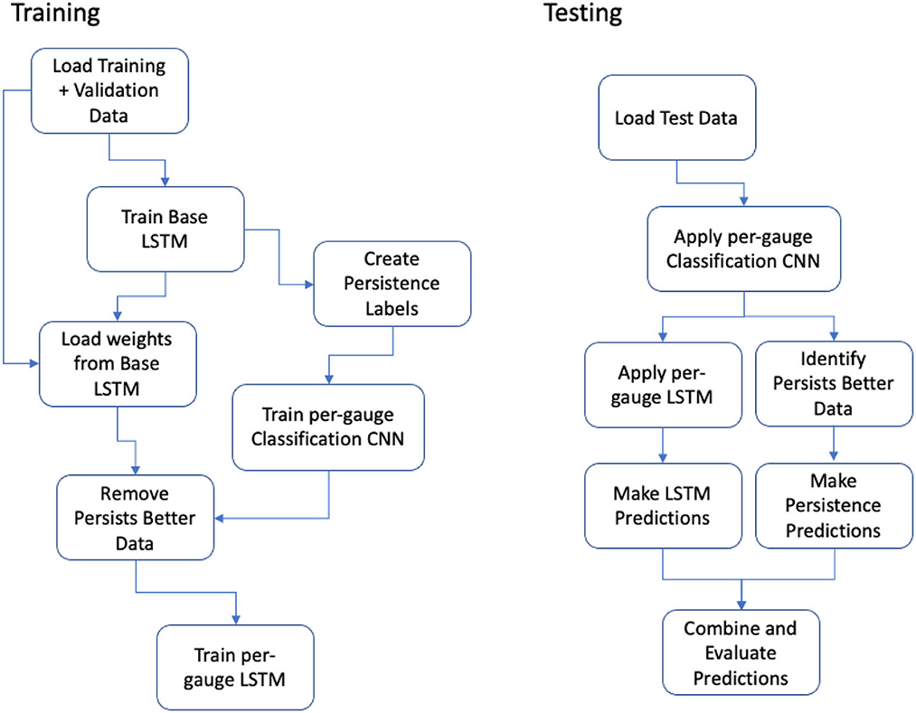
Figure 3. Sequence of model training and testing.

TABLE 1

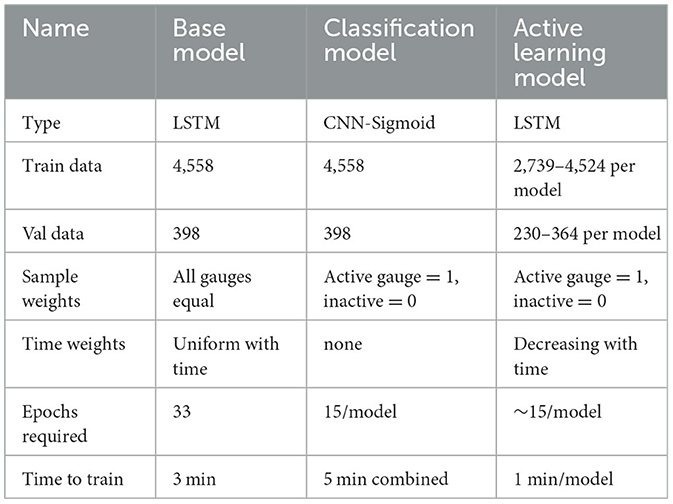
Table 1. Description of models used.

The slowest training step was creating the persistence labels which took 89 min. However, once created, these could be used for many different attempts at optimizing the per-gauge LSTM models.

3. Results

3.1. Model analysis

Various methods are commonly used to evaluate river flow forecast accuracy. Both the Nash and Sutcliffe (1970) method (Eq 1) and the dimensionless version of the Willmott et al. (2011) technique (Eq 2) were utilized here. The shortcomings of the most common methods including these two have been documented (Legates and McCabe, 1999; Jackson et al., 2019). One particular concern that has been raised before for the Willmott method is that it is benchmarked against the variance in past data. For the type of data examined here, this is especially problematic as the past variance can be zero for gauges near reservoirs and pipes. Unlike natural streams, reservoir levels, tunnel flows, and gauges directly connected to reservoir outflows can report zero past fluctuation for substantial periods of time. The Nash method suffers from lacking a lower bound and being strongly influenced by extreme outliers. While neural networks have used Nash as a minimization function, both Nash and Willmott were unsatisfying as loss functions for multiple reasons. MAE was found to be a more satisfying minimization and evaluation criteria although both Nash:

$\begin{array}{ll}E=1-\frac{{\displaystyle {\sum }_{i=1}^n{\left(P_i-O_i\right)}^2}}{{\displaystyle {\sum }_{i=1}^n{\left(O_i-\overline{O}\right)}^2}}& (1)\end{array}$

and Willmott error analysis:

$\begin{array}{l}1-\frac{{\displaystyle {\sum }_{i=1}^n\left|P_i-O_i\right|}}{c{\displaystyle {\sum }_{i=1}^n\left|O_i-\overline{O}\right|}}\text{ when}{\displaystyle {\sum }_{i=1}^n\left|P_i-O_i\right|}\le c{\displaystyle {\sum }_{i=1}^n\left|O_i-\overline{O}\right|} \\ \text{ and }\\ \frac{c{\displaystyle {\sum }_{i=1}^n\left|O_i-\overline{O}\right|}}{{\displaystyle {\sum }_{i=1}^n\left|P_i-O_i\right|}}-1\text{ when}{\displaystyle {\sum }_{i=1}^n\left|P_i-O_i\right|}>c{\displaystyle {\sum }_{i=1}^n\left|O_i-\overline{O}\right|}& (2)\end{array}$

MAE was found to be a more satisfying both Nash (Eq 1) and Willmott (Eq 2) analysis of the model using the set aside test data set are provided here. While the MAE is very direct and easily understandable, one drawback is that it is not scaled. As a result, gauges that have higher average flows tend to have predictions with larger MAE values. The impact of this scaling issue on using MAE for optimization is minimal. Most of the models described here are specific to a single gauge, so minimizing them based on errors on that gauge is not problematic. In the base model, all gauges are weighted equally, and higher flow gauges may disproportionately impact the gradient descent, but this base model is not used directly for predictions. Another consequence of using MAE is that when comparing predictions on the test data it can appear that gauges with higher average flow have larger errors. One common method to solve this is to scale errors using the mean absolute scaled error (MASE) (Hyndman and Koehler, 2006). However, the MASE would be infinite or undefined when recent historical observations are all equal in value, which is common for this type of data.

Each final LSTM model used a different number of days of data (out of a possible 4558) for training. While the initial training was performed on all 4,558 data sets, the classification allowed for curating the training set to contain only that data expected to help the most. The classification method when applied to selecting data used in the final model for each gauge ranged from 2,739 to 4,524 (Figure 4) out of the possible 4,558 days available. The gauges nearer water projects used the persistence model more frequently than the natural streams.

FIGURE 4

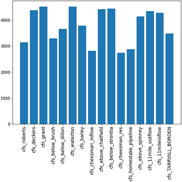
Figure 4. Number of days used in training final LSTM models.

When a 7-day prediction was run on 210 days of test data, the prediction 1 day into the future was close to that of the persistence model (Figure 5). In cases where there were rapid changes in flow, typically a rise, the convolutional LSTM model often was slower to show the increase. The convolutional LSTM models had mixed results when reservoirs or pipelines had long periods without any change. In some cases, such as below Dillon reservoir, this model was very similar to the persistence model. In other cases, such as homestake pipeline and cheesman reservoir, the convolutional LSTM model predicted flow at large sections of time when there was no flow recorded. Natural undammed streams such as below brush were reasonably accurate although the convolutional LSTM model was slower to respond to rapid changes. When run on the test data, the number of weeks labeled as being better modeled with persistence ranged from 98 to 133 out of the 210 days evaluated (yellow points in Figure 5).

FIGURE 5

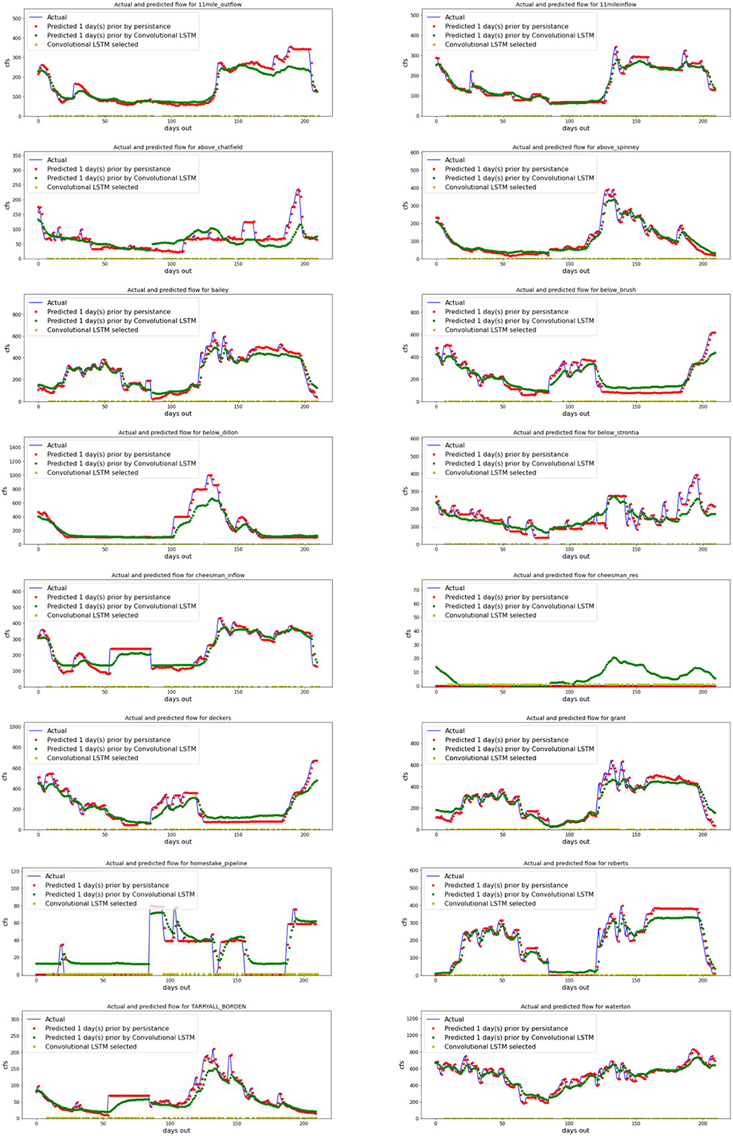
Figure 5. Two hundred and ten days of testing data where each gauge is modeled one day ahead using a persistence model and a gauge-specific convolutional LSTM for 2015 and 2016. A yellow square on the baseline indicates that the CNN classifier identified the convolutional LSTM as the better model based on the input past data. Blue line represents actual data, red the persistence model prediction, and green the convolutional LSTM prediction.

In the same 7-day prediction, the prediction 7 days into the future was not unexpectedly, less accurate than 1 day into the future (Figure 6). Again, when changes in flow were rapid, the convolutional LSTM model often was slower and did not rise as high as the actual flow (blue) or the persistence prediction (red). The convolutional LSTM models again overestimated flow at times when reservoirs or pipelines had long periods without any change such as in homestake, underestimated at other times as in Roberts tunnel, and identified small peaks below cheesman reservoir when the actual data had no such spike. Although the reservoir was undergoing repairs during this time period that may have caused it to deviate from the model prediction.

FIGURE 6

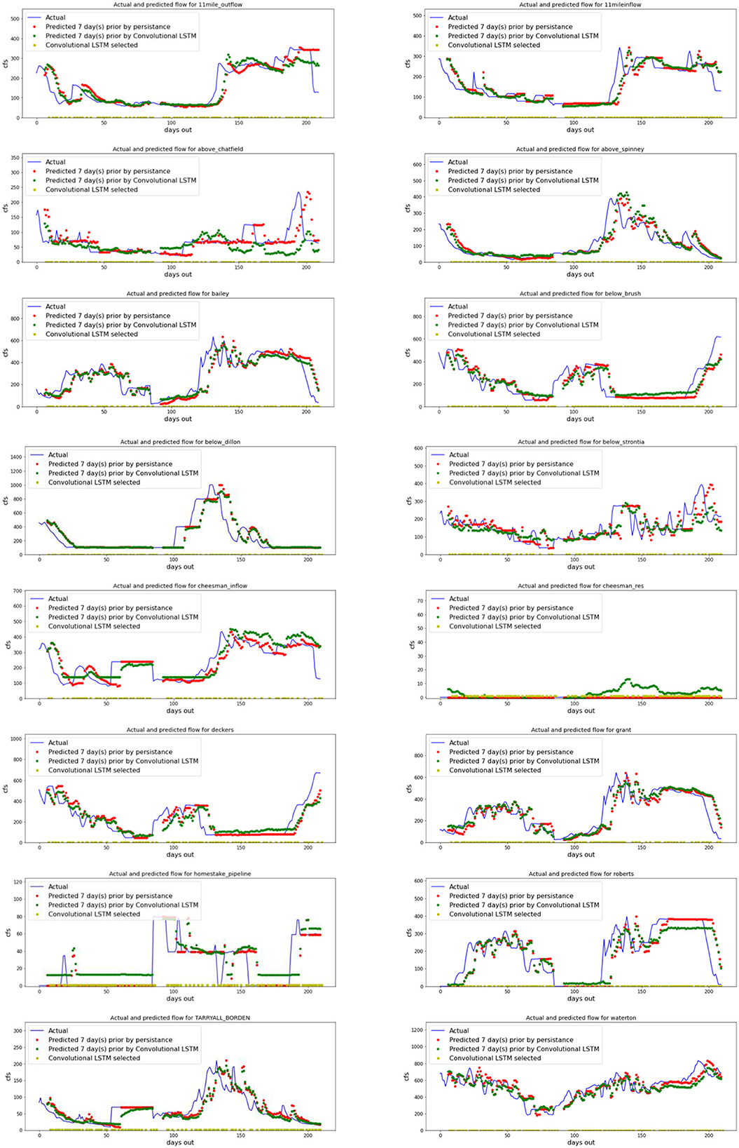
Figure 6. Two hundred and ten days of testing data where each gauge is modeled seven days ahead using a persistence model and a gauge-specific Convolutional LSTM for 2015 and 2016. A yellow square on the baseline indicates that the CNN classifier identified the Convolutional LSTM as the better model based on the input past data. Blue line represents actual data, red the persistence model prediction, and green the convolutional LSTM prediction.

The fully trained gauge specific models utilized approximately half of the available data provided from the classifier. These models trained on smaller datasets performed well at predicting flow from all the gauges. The median total error (sum of the absolute value of the difference between true value and predicted value for 7 future days combined) ranged from 0 cfs to as high as 413.7 cfs (Figure 7). The models with the higher flow gauges showed larger errors, as expected.

FIGURE 7

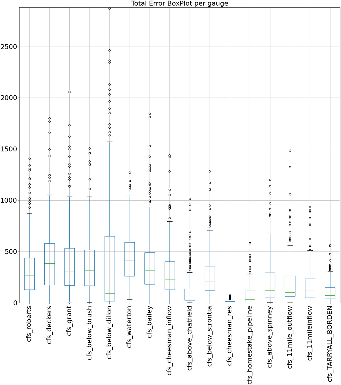
Figure 7. Combined absolute value of difference between predicted and actual values (in cfs) from 2015 and 2016 for 7 days of forecast combined.

When analyzing the test data (Figure 3, right) using this combination of classification CNN and convolutional LSTM predictor, the median Willmott values for all gauges ranged from 0.801 to 1.0 (Figure 8). Here the lowest values were for pipeline and reservoir gauges rather than natural river and stream flows.

FIGURE 8

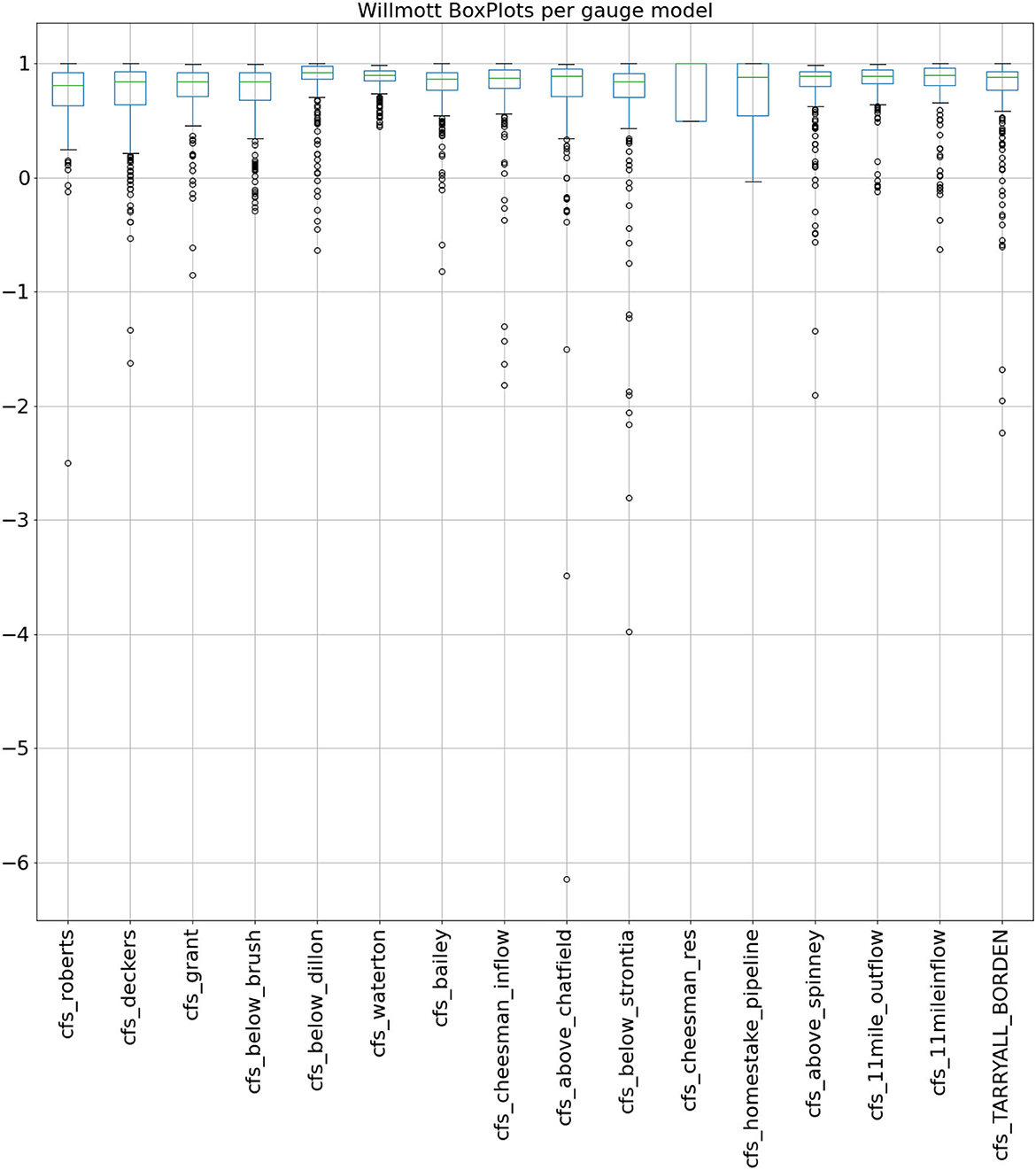
Figure 8. Error analysis on test data predictions from 2015 and 2016 using Willmott analysis.

The median Nash values for each gauge ranged from 0.65 to −5.39 with gauges close to reservoirs showing worse performance. Here the Nash values are graphed as a boxplot after removing outliers one standard deviation beyond the IQR (Figure 9).

FIGURE 9

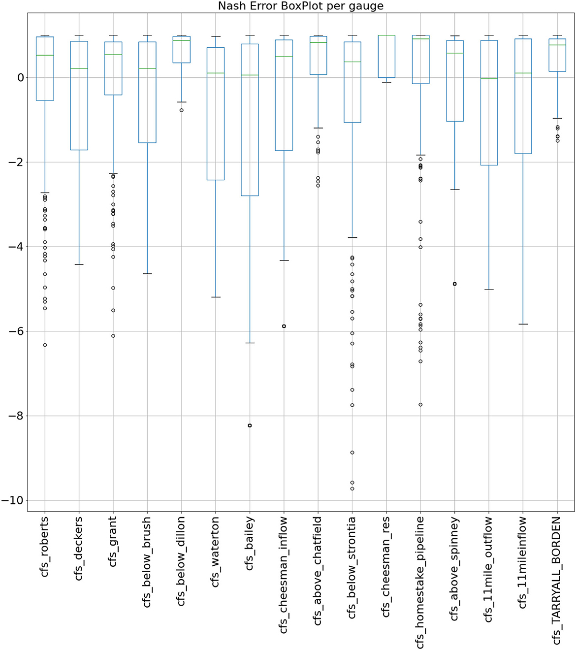
Figure 9. Nash-Sutcliffe analysis of test data predictions from 2015 and 2016.

Predictions were also made using the base model to allow for an analysis of the benefit of including the active learning and transfer learning into the overall model. In almost all cases, the final model performed better than the base model (Table 2) despite both being based on convolutional LSTM architecture, demonstrating that this approach does add to the forecast accuracy. The total error (over 7 days) was 11 to 196 cubic feet per second (cfs) better for the final model, all but two gauges had a better Willmott score, and all but 5 had a better Nash-Sutcliffe score. The propensity of Nash-Sutcliffe to overweight outliers likely impacted this result.

TABLE 2

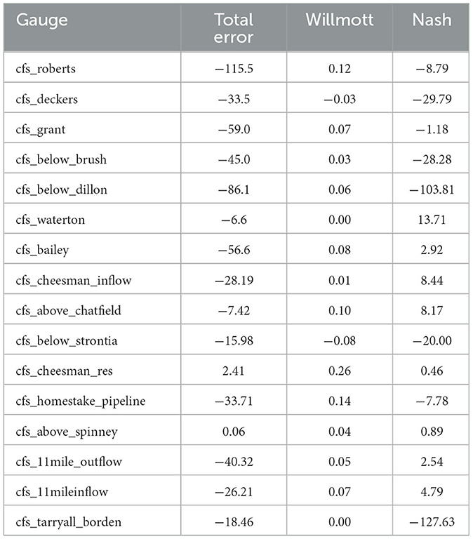
Table 2. Average difference between LSTM base and final models in three metrics for all testing data.

4. Discussion

A novel combination of neural networks was employed and in combination they provided more accurate predictions than a single convolutional LSTM model in isolation. The convolutional LSTM structure was a useful way to aggregate data from multiple inputs and to find patterns within those data sources while retaining time-based correlations within the data. The addition of a CNN based classifier to select data fed into the convolutional LSTM model training improved the accuracy of the predictions.

Unlike past ensemble methods, this is an on-the-fly approach where each dataset is examined to determine whether the characteristics of that dataset suggest the best method to fit the data. Two options are available although more could be added. Either the data is fit to a very simple persistence model or the data is fit to a convolutional LSTM. Yellow boxes in Figures 5, 6 reveal the granularity of this approach with model selection sometimes varying day by day and gauge by gauge.

Selection of an optimal model from among multiple models has long been performed using cross-validation (van der Laan et al., 2007). A more recent approach, the super ensemble method (Tyralis et al., 2021), combines multiple machine learning (ML) methods and applies a weighting to each method. This is computationally expensive as each ML method must be run even if it is determined that it merits an insignificant weighting. Also, this is not an on-the-fly method that adapts to different data inputs. If certain input data being used for a prediction is better suited to one of the aggregated ML methods than another, the weightings are not updated. Furthermore, hybrid methods have been developed (Di Nunno et al., 2023; Granata and Di Nunno, 2023) that combine both machine learning and deep learning methods to forecast streamflow. These also do not adapt to data on the fly.

The approach described here is a unique ensemble method although the selection is simply between two possible models (persistence or convolutional LSTM). Here only one of the two models is selected as opposed to the super ensemble approach which might be more suitable for combining multiple machine learning approaches. Here, if conditions are expected to result in no flow changes, a simple persistence model is the best possible predictor, so mixing in other methods might reduce the performance.

This approach is unique in that CNN convolutions of the data in the two dimensions the data is assembled and in the third dimension (time) are used to classify and thereby select a model to fit the data. This captures the same variability in data that is used in the LSTM based forecast. Unlike past ensemble methods, this is an on-the-fly approach where each analyzed dataset is examined to determine whether the characteristics of that dataset suggest the best method to fit the data with. Two options are available although more could be added. Local neighbors within the past states of the data determine the future states. In isolation, a CNN may seem like a heavy-handed method for characterizing data and selecting a model, however, the work of arranging the data into the structure necessary for analyzing by a CNN is already completed in preparation for analysis by the convolutional LSTM. We have not directly compared this classifies to other ensemble methods, which would be a worthwhile comparison, however, a more standard dataset may be more suitable to that analysis.

These models provide accurate predictions of flow both upriver and downriver of reservoirs and pipelines. These predictions could be useful to water users and water managers in modeling how individual decisions in one area effect other areas. Models of reservoir impacted streamflow have been proposed as a guide to support reservoir operations (Zhao and Cai, 2020) and have been modeled using machine learning (Huang et al., 2021). In addition to predicting flows, this method could be useful for modeling how to make changes to reservoir operations to account for climate change and other factors.

Other combinations could be used where a classifier selected data to be used in training later models in an active learning step. LSTM is one of many neural networks that can be used to predict future flows and classifier could be used to select between many different models.

5. Conclusions

The approach described here could be most suitable to forecasting in circumstances with large variation in inputs, such as extreme weather events. Combining multiple models that work under different circumstances allows monitoring for large changes while still using the best model available for more normal circumstances.

Predicting flow in rivers where human decision making is involved can only succeed when similar decisions were included in the training data. Singular events, such as repairs to a tunnel, or draw down of a reservoir for repairs may occur too infrequently to be modeled within the training data. One missing variable, in particular, are water calls made by downstream users. These calls may be made based on weather conditions far outside the river basin and add to uncertainty in these predictions.

The approach used here improves prediction accuracy but does so with an increase in complexity. Many different neural networks are used, and the process of transfer learning increases this complexity. Making changes to the data processing in this format can be challenging. It is not possible for example to drop a single gauge part way through the process, although weights can be used to minimize the influence of that gauge.

Optimizing a combination of neural networks such as this is complicated. Relatively minimal effort has been made to fully optimize all the possible hyperparameters because of this. Specifically, a few different regularization values and batch sizes were explored in the base LSTM model. Once selected, these values were used throughout with all subsequent models. Methods are available to systematically explore hyperparameters (Dumont et al., 2021), however, it would take significant adaptation to use these approaches and to allow the hyperparameters to vary between models.

This approach could be employed recursively by creating a new classifier not from the base LSTM but from the active-learning improved LSTMs. In turn, these LSTMs could again be used to create new classifiers to better select training data to be used in another round of training in a recursive manner.

Data availability statement

Publicly available datasets were analyzed in this study. This data can be found here: https://dwr.state.co.us/Rest/GET/Help and details on the specific data used in this study can be found here: https://github.com/scottmreed/Active-Learning-CNN-for-Predicting-River-Flow.

Author contributions

SR: Conceptualization, Methodology, Software, Visualization, Writing.

Funding

The author(s) declare that no financial support was received for the research, authorship, and/or publication of this article.

Conflict of interest

The author declares that the research was conducted in the absence of any commercial or financial relationships that could be construed as a potential conflict of interest.

Publisher's note

All claims expressed in this article are solely those of the authors and do not necessarily represent those of their affiliated organizations, or those of the publisher, the editors and the reviewers. Any product that may be evaluated in this article, or claim that may be made by its manufacturer, is not guaranteed or endorsed by the publisher.

References

Anguita, J. G. M., and Olariaga, O. D. (2023). Air cargo transport demand forecasting using ConvLSTM2D, an artificial neural network architecture approach. Case Stud. Transp. Policy 12, 101009. doi: 10.1016/j.cstp.2023.101009

CrossRef Full Text | Google Scholar

Chiacchiera, A., Sai, F., Salvetti, A., and Guariso, G. (2022). Neural Structures to Predict River Stages in Heavily Urbanized Catchments. Water, 14, 2330. doi: 10.3390/w14152330

CrossRef Full Text | Google Scholar

Di Nunno, F., de Marinis, G., and Granata, F. (2023). Short-term forecasts of streamflow in the UK based on a novel hybrid artificial intelligence algorithm. Sci. Rep. 13, 7036. doi: 10.1038/s41598-023-34316-3

PubMed Abstract | CrossRef Full Text | Google Scholar

Duan, S., Ullrich, P., and Shu, L. (2020). Using convolutional neural networks for streamflow projection in California. Front. Water 2, 28. doi: 10.3389/frwa.2020.00028

CrossRef Full Text | Google Scholar

Dumont, V., Garner, C., Trivedi, A., Jones, C., Ganapati, V., Mueller, J., et al. (2021). HYPPO: a surrogate-based multi-level parallelism tool for hyperparameter optimization. In: IEEE/ACM Workshop on Machine Learning in High Performance Computing Environments (MLHPC), St. Louis, MO, 81–93.

Google Scholar

Fang, Z., Xie, J., Peng, R., and Wang, S. (2021). Climate finance: mapping air pollution and finance market in time series. Econometrics 9, 43. doi: 10.3390/econometrics9040043

CrossRef Full Text | Google Scholar

Fu, G., Jin, Y., Sun, S., Yuan, Z., and Butler, D. (2022). The role of deep learning in urban water management: a critical review. Water Res. 223, 118973. doi: 10.1016/j.watres.2022.118973

CrossRef Full Text | Google Scholar

Gikunda, P., and Jouandeau, N. (2021). Homogeneous transfer active learning for time series classification. In: 2021 20th IEEE International Conference on Machine Learning and Applications (ICMLA), Pasadena, CA, 778–784.

Google Scholar

Granata, F., and Di Nunno, F. (2023). Neuroforecasting of daily streamflows in the UK for short- and medium-term horizons: a novel insight. J. Hydrol. 624, 129888. doi: 10.1016/j.jhydrol.2023.129888

CrossRef Full Text | Google Scholar

Huang, R., Ma, C., Ma, J., Huangfu, X., and He, Q. (2021). Machine learning in natural and engineered water systems. Water Res. 205, 117666. doi: 10.1016/j.watres.2021.117666

PubMed Abstract | CrossRef Full Text | Google Scholar

Hyndman, R. J., and Koehler, A. B. (2006). Another look at measures of forecast accuracy. Int. J. Forecast. 22, 679–688. doi: 10.1016/j.ijforecast.2006.03.001

CrossRef Full Text | Google Scholar

Jackson, E. K., Roberts, W., Nelsen, B., Williams, G. P., Nelson, E. J., and Ames, D. P. (2019). Introductory overview: error metrics for hydrologic modelling A review of common practices and an open source library to facilitate use and adoption. Environ. Model. Software 119, 32–48. doi: 10.1016/j.envsoft.2019.05.001

CrossRef Full Text | Google Scholar

Kratzert, F., Klotz, D., Brenner, C., Schulz, K., and Herrnegger, M. (2018). Rainfallrunoff modelling using Long Short-Term Memory (LSTM) networks. Hydrol. Earth Syst. Sci. 22, 6005–6022. doi: 10.5194/hess-22-6005-2018

CrossRef Full Text | Google Scholar

Le, X. -H., Nguyen, D. -H., Jung, S., Yeon, M, and Lee, G. (2021). Comparison of deep learning techniques for river streamflow Forecasting. IEEE Access 9, 71805–71820. doi: 10.1109/ACCESS.2021.3077703

CrossRef Full Text | Google Scholar

Legates, D. R., and McCabe, G. J. (1999). Evaluating the use of goodness-of-fit measures in hydrologic and hydroclimatic model validation. Water Res. Res. 35, 233–241. doi: 10.1029/1998WR900018

CrossRef Full Text | Google Scholar

Liu, W., Wang, Y., Zhong, D., Xie, S., and Xu, J. (2022). ConvLSTM network-based rainfall nowcasting method with combined reflectance and radar-retrieved wind field as inputs. Atmosphere 13, 411. doi: 10.3390/atmos13030411

CrossRef Full Text | Google Scholar

MacDonnell, L. (2023). The 1922 Colorado River Compact at 100. Western Legal History. p. 33. Available online at: https://ssrn.com/abstract=4526135 (accessed August 2, 2023).

Google Scholar

Moishin, M., Deo, R. C., Prasad, R., Raj, N., and Abdulla, S. (2021). Designing deep-based learning flood forecast model with ConvLSTM hybrid algorithm. IEEE 9, 50982–50993. doi: 10.1109/ACCESS.2021.3065939

CrossRef Full Text | Google Scholar

Nash, J. E., and Sutcliffe, J. V. (1970). River flow forecasting through conceptual models part I A discussion of principles. J. Hydrol. 10, 282–290. doi: 10.1016/0022-1694(70)90255-6

CrossRef Full Text | Google Scholar

Poornima, S., and Pushpalatha, M. (2019). Prediction of rainfall using intensified LSTM based recurrent neural network with weighted linear units. Atmosphere 10, 668. doi: 10.3390/atmos10110668

CrossRef Full Text | Google Scholar

Ren, P., Xiao, Y., Chang, X., Huang, P.-Y., Li, Z., Gupta, B. B., et al. (2021). A survey of deep active learning. ACM Comput. Surv. 54, 1–40. doi: 10.1145/3472291

CrossRef Full Text | Google Scholar

Sagheer, A., and Kotb, M. (2019). Unsupervised pre-training of a deep LSTM-based stacked autoencoder for multivariate time series forecasting problems. Sci. Rep. 9, 19038. doi: 10.1038/s41598-019-55320-6

PubMed Abstract | CrossRef Full Text | Google Scholar

Schultz, M. G., Betancourt, C., Gong, B., Kleinert, F., Langguth, M., Leufen, L. H., et al. (2021). Can deep learning beat numerical weather prediction? Philos. Trans. A Math. Phy. Eng. Sci. 379, 20200097. doi: 10.1098/rsta.2020.0097

PubMed Abstract | CrossRef Full Text | Google Scholar

Shi, X., Chen, Z., Wang, H., Yeung, D. Y., Wong, W. K., and andWoo, W. C. (2015). Convolutional LSTM network: a machine learning approach for precipitation nowcasting. Adv. Neural Inform. Proc. Syst. 28, 802–810.

Google Scholar

Shu, X., Ding, W., Peng, Y., Wang, Z., Wu, J., and Li, M. (2021). Monthly streamflow forecasting using convolutional neural network. Water Resour. Manage. 35, 5089–5104 doi: 10.1007/s11269-021-02961-w

CrossRef Full Text | Google Scholar

Sit, M., Demiray, B. Z., Xiang, Z., Ewing, G. J., Sermet, Y., and Demir, I. (2020). A comprehensive review of deep learning applications in hydrology and water resources. Water Sci. Technol. 82, 2635–2670. doi: 10.2166/wst.2020.369

PubMed Abstract | CrossRef Full Text | Google Scholar

Tyralis, H., Papacharalampous, G., and Langousis, A. (2021). Super ensemble learning for daily streamflow forecasting: large-scale demonstration and comparison with multiple machine learning algorithms. Neural Comput. Appl. 33, 3053–3068. doi: 10.1007/s00521-020-05172-3

CrossRef Full Text | Google Scholar

van der Laan, M. J., Polley, E. C., and Hubbard, A. E. (2007). Super learner. Stat. Appl. Genet. Mol. Biol. 6, 25. doi: 10.2202/1544-6115.1309

CrossRef Full Text | Google Scholar

van der Lugt, B. J., and Feelders, A. J. (2020). “Conditional forecasting of water level time series with RNNs” in Advanced Analytics and Learning on Temporal Data, (Berlin: Springer International Publishing), 55–71.

Google Scholar

Willmott, C. J., Robeson, S. M., and Matsuura, K. (2011). A refined index of model performance. Int. J. Climatol. 32, 2088–2094. doi: 10.1002/joc.2419

CrossRef Full Text | Google Scholar

Xiang, Z., Yan, J., and Demir, I. (2020). A rainfall-runoff model with LSTM-based sequence-to-sequence learning. Water Res. Res. 56, e2019WR025326. doi: 10.1029/2019WR025326

CrossRef Full Text | Google Scholar

Zhao, Q., and Cai, X. (2020). Deriving representative reservoir operation rules using a hidden Markov-decision tree model. Adv. Water Res. 146, 103753. doi: 10.1016/j.advwatres.2020.103753

CrossRef Full Text | Google Scholar