Rainfall Patterns From Multiscale Sample Entropy Analysis

Precipitation is a manifestation of many interacting complex processes. How to grasp its temporal pattern that would reveal underlain dominant contributing factors is the key objective of the study. For this, we explored the application of multiscale sample entropy (MSE) in describing the long-term daily precipitation. Sample entropy (SE) adds similarity measure over the conventional information entropy, and it has been used in quantifying changing complexity in chaotic dynamic systems. With the further incorporation of multiscale consideration, the MSE analysis gives the trend of SE changes with scale, and provides a rich description of participating factors. The daily precipitation time series studied were taken from 665 weather stations across China that have been recorded for about 50–61 years. The SE estimates are a function of the length of time series (n), the dimension of similarity (m), and the match threshold (r). These parameters are problem-dependent, and through simulation, this study has determined that m = 2, r = 0.15, and n ≈ 20,000 would be appropriate for estimating SE up to the 30-day scale. Three general patterns of MSE for precipitation time series are identified: (1) Pattern A, SE increases with scale; (2) Pattern B, SE increases then decreases and followed by increase; and (3) Pattern C, SE increases then decreases. The MSE is found capable of detecting differences in characteristics among precipitation time series. Matching MSE thus could serve as a metric to evaluate the adequacy of simulated precipitation time series. Using this metric, we have shown that to embody seasonal changes one needs to use different monthly two-parameter gamma distribution functions in generating simulated precipitation time series. Moreover, for dry seasons, one also needs to consider interannual fluctuations: it is inadequate to use just one single function for simulating multi-year precipitation data. Finally, for the study region, MSE patterns show coherence over the distance in that stations that are close, which range from 40 to 80 km, exhibit similar MSE trends. The MSE patterns obtained are also found to be reflective of the regional precipitation patterns—this has important implications on water resources management.

Introduction

Precipitation is a manifestation of many interacting complex processes. It is one of the most volatile and unpredictable climate variables in most parts of the world. The high variability of precipitation, both in time and space, has tremendous impacts on agriculture, food security, and the management of water resources. To improve our understanding of the characteristics of the precipitation over different regions of the world, it is critically important to investigate the precipitation variability and its associated temporal and spatial trends and patterns. Traditionally, the probability functions are used in describing the characteristics of the precipitation for locations where the precipitation time series are often deemed stationary. For example, the statistical distributions are used for the daily rainfall to study the rainfall regimes in Europe (Burgueno et al., 2010) and in Western Orissa (Mangaraj and Sahoo, 2010). Ghosh (2010) used the copula distribution to study the bivariate rainfall distribution. However, due to the complexity involved in the precipitation, there are no explicit conditions under which the typically known statistical distributions would always perform well at all locations. Moreover, there are no sets of formulations with which the precipitation can be perfectly described, especially with the changing climate where the stationary assumptions are invalid (Quintero et al., 2018; Lawrence, 2020; Silva et al., 2021; Slater et al., 2021). Thus, various approximations and assumptions have to be made, such as independence among precipitation data in nearby stations within study regions.

Entropy, in contrast, is a good measure of variability when the probability distribution of a variable is not symmetric (e.g., Singh, 1997; Avseth et al., 2005). It has also been shown that entropy may be related to higher order moments of a distribution and thus it offers a closer characterization of a distribution (e.g., Ebrahimi, 1999). As entropy is useful in quantifying randomness of processes, there are a large number of studies where entropy was employed to study the rainfall characteristics including temporal and spatial patterns. For example, Kawachi et al. (2001) used the average of annual entropies and median of annual rainfalls to categorize the rainfall stations in Japan and constructed a water availability map. Maruyama et al. (2005) used the intensity entropy and apportionment entropy to understand the monthly rainfall variability around the world. Using entropy to measure the rainfall variability of different timescales (monthly, seasonal, yearly, and decadal), Mishra et al. (2009) concluded that the increasing trends of drought in some regions may continue in Texas, USA. Brunsell (2010) employed entropy to investigate the spatial and temporal variability of daily precipitation over the continental U.S. Brunsell's results show a breakpoint in the central plains due to the presence of the Rocky Mountains, demonstrating the benefits of using entropy to identify features that are not readily identifiable from the time series data. Hasan and Dunn (2011) used entropy to quantify the rainfall variability in Australia in which the long-term average of rainfall amounts across the months of the year is used. Extending the original use of entropy by Amorocho and Espidora (1973), Liu et al. (2013) constructed an entropy model to analyze the large-scale rainfall distribution in the Pearl River Basin in China based on monthly rainfall data from 1959 to 2009 over 62 stations. In the aforementioned studies, the conventional information entropy is employed and applied to one timescale in each application, either to daily, monthly, seasonal, or yearly; a few have repeated the calculation to monthly, seasonal, yearly, and decadal scales (Mishra et al., 2009).

The concept of sample entropy (SE) has been shown promising in identifying changes in complexity (Richman and Moorman, 2000) of a chaotic dynamic system. It has been applied to study spatial and temporal patterns and trends of precipitation and runoff (e.g., Khan et al., 2016; Li et al., 2017; Xavier et al., 2019; Zhang et al., 2020). Zhang et al. (2019) investigated the spatiotemporal differences of monthly precipitation complexity in Heilongjiang Province, China and found that the SE is more suitable for analyzing precipitation complexity than the fuzzy entropy, wavelet entropy, and permutation entropy as the SE provided more stable and reliable results. The SE differs from the conventional information entropy for it has taken into account the dimensional similarity. Of particular interests is the evidence showing that the multiscale sample entropy (MSE) can consistently identify the loss of complexity in a biological time series (Costa et al., 2005). This finding is the main impetus of the present study. Li and Zhang (2008) applied MSE to investigate the possible change in complexity of the Mississippi River due to human activities such as the practices in land use and land cover. They showed that there was a loss in complexity in the Mississippi River flow around 1940. However, the application of MSE to study the spatiotemporal patterns of precipitation has been quite limited. Chou (2011) applied MSE to help determine the number of resolution levels used in wavelet decomposition analysis. Chou (2014) did a preliminary study of applying MSE to both the rainfall and streamflow time series in Taiwan where Chou found that the complexity of rainfall is different from that of the streamflow. Chou also found that the daily and annual data in the analysis showed low complexity and high predictability and thus recommended to use MSE to identify the temporal scales with low complexity. Alves Xavier et al. (2021) have found that the MSE can distinguish rainfall regimes between the inland semiarid and the coastal, tropical humid regions based on 69 meteorological stations from Brazil. The MSE is also shown capable of revealing the complexity of precipitation time series that varies spatially in an urban setting (Liu et al., 2018).

So far, the application of MSE to study precipitation data are mostly based on monthly records and over small regions; there is a knowledge gap in the fundamental understanding of whether MSE of precipitation is related to the underlain factors which impact its shape and behavior. Conversely, a systematic and comprehensive study of MSE from a large set of precipitation records allows us to address a long-standing challenging question, “Could precipitation temporal patterns reveal underlain dominant contributing factors?”

To the best of our knowledge, this study is the first of its kind to present a framework to extract essential characteristics contained in the observed precipitation time series to systematically generate complex non-stationary daily precipitation time series, guided by MSE, that considers interannual variability using precipitation statistical distributions. This study addresses the following fundamental and critical questions: First, are there precipitation patterns one can readily identify in terms of MSE and associate them with climates? Second, if there are clear precipitation MSE patterns, what are the dominate factors leading to such patterns? Third, would the use of MSE complement the common use of the two-parameter gamma distribution in providing better ways to describe precipitation and its simulation?

To address the preceding questions, the selection of appropriate parameters for determining MSE is tackled first as they are problem-dependent and needs to be resolved. Following that, this study investigates a large set of precipitation data that have collected over a large area and over a long period of time, and look for the patterns in MSE and their spatial variation. Then the focus is on if the MSE could discern the characteristics embedded in long-term precipitation data, and on if MSE could serve as a useful measure that allows one to identify the dominating factors among all the interacting complex processes that shape the precipitation characteristics as observed.

MSE

SE in a Nutshell

The SE, as presented by Richman and Moorman (2000), is an improvement over the approximate entropy (Pincus, 1991) that was developed to quantify changing complexity in chaotic systems. In a nutshell, SE introduces a correlation or similarity dimension into the entropy computation in determining the “orderliness” contained in a time series. The core of SE is the conditional probability that two sequences that are similar for m consecutive points remain similar when each sequence is extended by one additional point. The SE is defined as the negative natural logarithm of this conditional probability. The estimation of SE thus depends on the following three factors: The length of a time series (n); the length of the data sequence to be compared (m); and the tolerance (r) for accepting matches. This r parameter sets the tolerance of match as r × SD_X, known as r-matched, where SD_X is the standard deviation of the time series, X. In a multiscale case, the scale one standard deviation is used for all scales. A brief description of the procedure for computing the SE is given below.

From a precipitation time series of length n, X_o = [x₁, x₂, …, x_n], a new time series is constructed by taking continuous m-point samples. Denoting a consecutive m-point sample starts at x_i as a vector X_i, namely, X_i = [x_i, x_i+1, …, x_i+m−1], the resulting new time series, X, can be expressed as follows:

$\begin{array}{ll}X=\left[X_1,X_2,\dots ,X_{n-m+1}\right]& (1)\end{array}$

Two vectors X_i and X_j are considered r-matched if the maximum differences between their corresponding elements are smaller than the r tolerance. That is, X_i and X_j are r-matched if max|X_i − X_j| ≤ r × SD_Xo. For computing the conditional probability of SE, the probability that two vectors of same length are r-matched is estimated first. For that, the number of X_j vectors, with j ≠ i, that are r-matched with X_i, is counted and divided by n – m, the number of pairs compared. This is denoted as ${B_i}^m(r)$. This count is repeated for every X_i, and the probability that any two vectors of length, m, would match is estimated as a normalized sum, denoted as B^m(r), which equals $1/(n-m+1){\displaystyle \sum _{i=1}^{n-m+1}}{B}_i^m$. In a similar fashion, B^m+1(r) is obtained for vectors of length, m + 1. The conditional probability of two m-length vectors that match remain matched when one additional point is added to each vector thus equals B^m+1(r)/B^m(r). From these terms, the SE is defined per m and r as follows:

$\begin{array}{ll}SE(m,r)={\displaystyle \underset{n\to \infty }{lim}}-ln\frac{B^{m+1}(r)}{B^m(r)}& (2)\end{array}$

In applications to a time series of a finite length, an estimate SE(m, r) is obtained without taking the limit and is written as SE(m, r, n). The length n that is needed to give a reasonable estimate of SE depends on the nature of the time series and the level of r adopted. This is investigated first for the study of precipitation data.

MSE Essentials

In processing physical and physiologic time series, Lake et al. (2002) have found that the impact of certain processes underlying a time series could only be discovered when SE estimates were viewed simultaneously across a wide range of scales. An upscaling represents an averaging process or a coarsened view of the original time series. For the scale k, the time series is averaged within a non-overlapping contiguous windows of width k, and has its length reduced to n/k in contrast to the original length of n at scale 1. Each element in the k-scale time series is obtained as

$\begin{array}{ll}{y}_i^k=1/k{\displaystyle \sum _{j=i}^{i+k-1}}{x}_j,& (3)\end{array}$

The fact that a multiscale SE, or MSE, representation of a time series could be useful in revealing the underlying processes involved is illustrated in Figure 1. In Figure 1A, time series generated by three well-known stochastic processes are presented: They are a fractional Brownian noise, a 1/f noise and a white noise. Here, each of the time series at scale one consists of 20,000 points. Figure 1B presents the MSE obtained for them, which was computed using m = 2, r = 0.15. For the white noise, its SE exhibits a monotonic decrease with scale as expected since the averaging process reduces the randomness and increases its orderliness. The 1/f noise is self-similar, or fractal, and by its nature possesses the same characteristics at different scales. That is clearly reflected in its SE not changing with scale. The fractional Brownian noise is self-affine. For the fractional Brownian noise, when Hurst index, H, is <0.5, the Brownian noise contains short range dependence, whereas when H is >0.5 it has long-range dependence, or long-term memory. Here, it is used to illustrate the point that that memory or dependence range in a time series affects its trend of the SE with scale. This can be observed from Figure 1C in which an example of the MSE of fractional Brownian noises with H varies from 0.1 to 0.9 are presented.

FIGURE 1

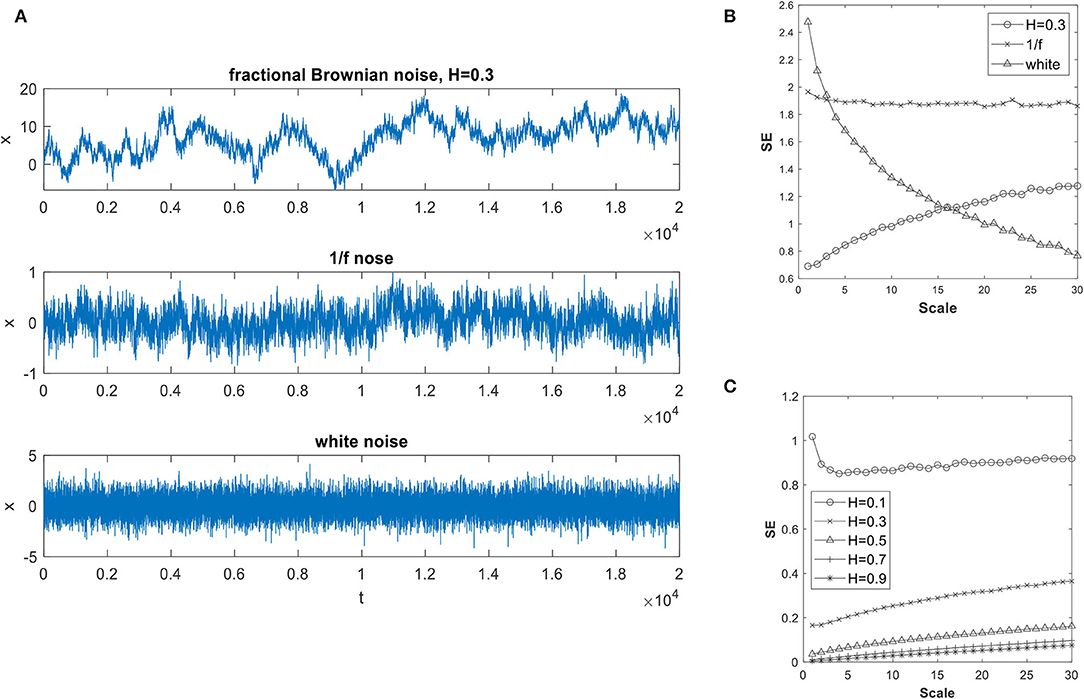
Figure 1. (A) Sample time series generated with Fractional Brownian noise, 1/f noise and white noise; (B) Variation of sample entropy with scales of the three time series; and (C) How the Hurst index of a fractional Brownian noise affects sample entry.

The fact that the MSE could be used in distinguishing time series from the different processes as shown in Figure 1 is one of the impetuses for investigating its use in analyzing the precipitation data. We start the study by first investigating the parameters to be used for the SE computation.

Parameter Selection for Computation of SE

As per its definition, the SE estimates are affected by the three parameters m, r, and n as discussed. The appropriate values for these parameters are problem-dependent. Since there is no baseline information existed for computing SE for the precipitation time series, a detailed numerical study is conducted. The m, r, and n parameter values to be adopted should result in small errors in the SE estimates. As the first step, we first determine the precipitation probability distribution functions using recorded data from weather stations. We then generated simulated precipitation time series based on the derived probability distribution function and its parameters. Then the variances of SE are computed over a range of m, r, and n values.

Characterization of the Precipitation Data

In this study, the daily precipitation data were obtained from the Chinese Scientific Data Sharing Network. The long data time series from 665 weather stations and the corresponding spatial distribution are shown in Figure 2. The precipitation time series used are at least 50 years long. Among them, we have used 61 years of records from 252 stations; 55–60 years of records from 327 stations; and 50–55 years of records from 86 stations. These data were acquired by recording the 24-h accumulated precipitation at 8 pm each day with an accuracy of ±0.1 mm.

FIGURE 2

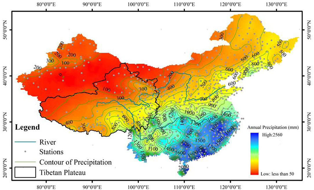
Figure 2. Map covers only the study area where weather stations are located with contours of average annual precipitation in mm.

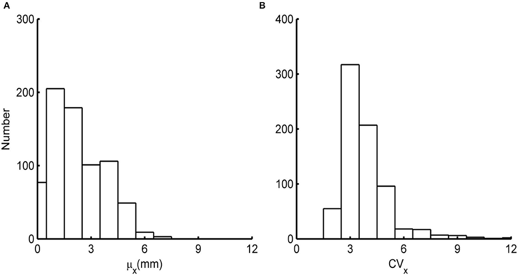
As the first step, we evaluate the goodness of fit of various probability distribution functions for the whole available length of daily precipitation data from each station. Among all the probability distribution functions evaluated, including but not limited to lognormal, three-parameter gamma, and generalized Pareto distributions, the two-parameter gamma distribution fits the data set best of all according to L-moment statistics as illustrated by the L-Kurtosis vs. L-Skewness plot of Figure 3 (Martinez-Villalobos and Neelin, 2019). The histograms of the means, μ_X, and the coefficients of variation, CV_X, from all the data are presented in Figure 4. It can be observed that the daily mean precipitation varies over a wide range reflecting the large area over which the stations span.

FIGURE 3

Figure 3. L-statistics of fitted gamma distribution for all 665 records used.

FIGURE 4

Figure 4. Histogram for daily (A) μ_X and (B) CV_X of 665 precipitation records studied.

The characteristics reflected in the two-parameter gamma distribution are used in generating data for quantifying variability of MSE estimates caused by differences in controlling parameters. Specifically, simulated precipitation time series are generated with daily mean, μ_X, varying from 1 to 11 mm and with CV_X varying from 0.5 to 8.

Determining m and r

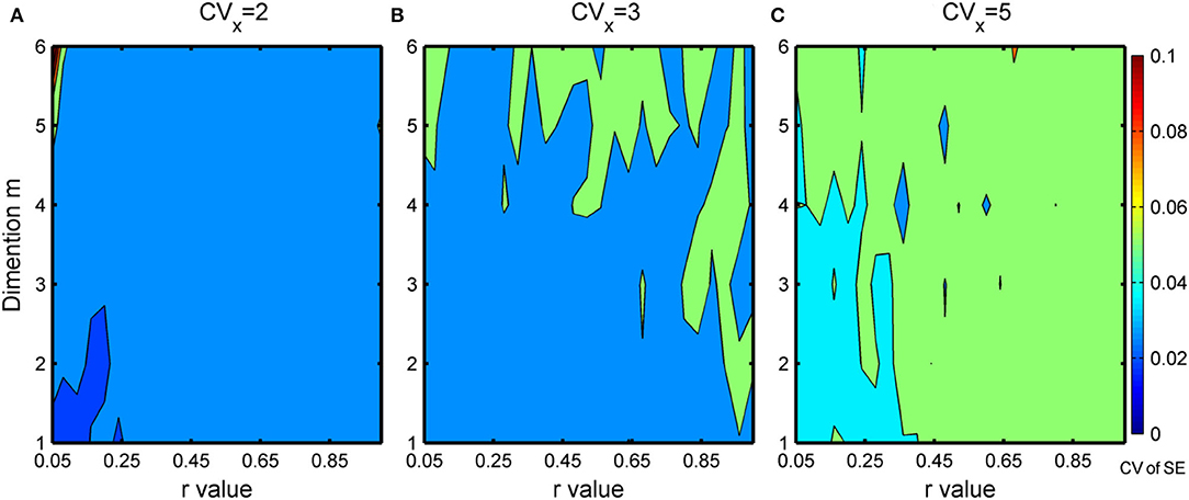
For each set of μ_X and CV_X, 50 simulated gamma-distributed time series are generated with each having a length, n = 20,000. The SE are then computed by varying m from 1 to 6 and r from 0.05 to 0.95. The acceptable m and r values are those that lead to small CV in SE estimates. In this study, this threshold CV is set to be 5%. In general, as illustrated in Figure 5, the higher the values of m and r are, the larger the CV of SE. From the figure, we found that the commonly used m of 2 and r of 0.15 (Costa et al., 2005; Chou, 2012, 2014) to be satisfactory for estimating SE from precipitation time series. This is consistent with recent findings (e.g., Li et al., 2017; Liu et al., 2018; Zhang et al., 2020) which show that stable and/or optimal results were obtained when m = 2 and r is between 0.1 and 0.25 times of the standard deviation.

FIGURE 5

Figure 5. (A–C) Variation of CV of SE with respect to r and m under different CV_X levels.

Determining the Minimum Length of Time Series

Our results further show that with a given CV_X, the CV of SE reduces as expected when the length n increases but stabilizes when n is sufficiently large as shown in Figure 6. Conversely, n has to be increased to maintain the same CV of SE if CV_X of the time series increases.

FIGURE 6

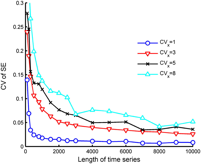
Figure 6. Variation of CV of SE with respect to length and CV_X of the time series (m = 2, r = 0.15).

As per the requirement, the length, n, needs to be sufficiently long so that CV of SE is limited to 5%, we found a linear relationship between n and CV_X based on Figure 6 as follows:

$\begin{array}{ll}n=1010·C{V}_X-810for1\le C{V}_X\le 10& (4)\end{array}$

For a gamma time series with CV_X = 8, a reasonable estimate of SE requires it to have a length of at least 7,270. However, to estimate the minimum length required of a time series at a higher scale, one needs to consider the reduction of the CV_X with scale which can be written readily as $C{V}_X^{Scale}=C{V}_X/\sqrt{scale}$. From this, at the scale 30, CV_X would decrease from 8 to $8/\sqrt{30}=1.46$, and the length of points required at that scale is around 665. To satisfy this, the number of data at scale 30 would require the time series at scale 1 to be about 665 × 30, or close to 20,000 points. This has an important bearing for the study as discussed in the following: As the precipitation data we are studying have CV_X mostly below 8, it follows that we could estimate SE reasonably well up to a scale 30 from 50 or more years of recorded daily precipitation data.

MSE of Gamma-Distributed Precipitation

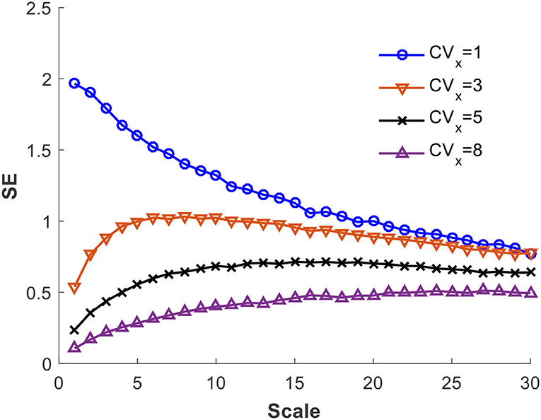
We computed MSE of simulated precipitation time series: each has n = 20,000 points and is generated using the gamma distribution function with a set of daily μ_X and CV_X. Using m = 2 and r = 0.15, we found that the MSE is sensitive to CV_X but not to μ_X. This point is illustrated in Figure 7 in which μ_X = 3 mm/day. From the figure, it can readily be observed that when CV_X is small, the SE variation with scale is similar to that of the white noise. On the other hand, when CV_X is high, the trend resembles that of a long memory fractional Brownian noise. The time series with intermediate CV_X give MSE with trends that lie in-between the preceding two. This demonstrates that the gamma-distributed time series exhibits rich behavior and explains why it is versatile in fitting precipitation time series. The discussion that follows further sheds light on the application of gamma distribution in describing recorded data.

FIGURE 7

Figure 7. MSE patterns versus CV_X of simulated gamma distributed time series with μ_X = 3.

MSE Patterns of Precipitation Time Series

The daily precipitation MSE is computed for each of the long records from the 665 weather stations used. Despite individual variations, three distinct MSE patterns, denoted as Pattern A, Pattern B, and Pattern C, are identified as shown, respectively, in Figures 8A–C. The SE variation with scales exhibits the following characteristics: (1) Pattern A shows a steady increasing trend throughout the scales with the rate of increase gradually reduces after the initial fast pace of change and becomes either flat or with a small upward trend at the end; (2) Pattern B shows a steady increasing trend which is interrupted by a reduction over several scales before returned to rise again; and (3) Pattern C first shows a steady increase trend that is followed by a steady decrease trend. From this figure, it can also be observed that all these three patterns show an initial increase in the SE up to about the scale of 5-day. This rising phase could be shorter and has been observed for as short as the 1-day scale. This initial rising phase of SE can readily be explained: Each of the daily precipitation time series is populated with days of mostly small to no precipitation, and, as such, they are initially similar. The similarity, however, is destroyed when more days are combined together in a coarsened view, which explained the rise in the SE as the orderliness of no rain in the initial scales is gradually decreased.

FIGURE 8

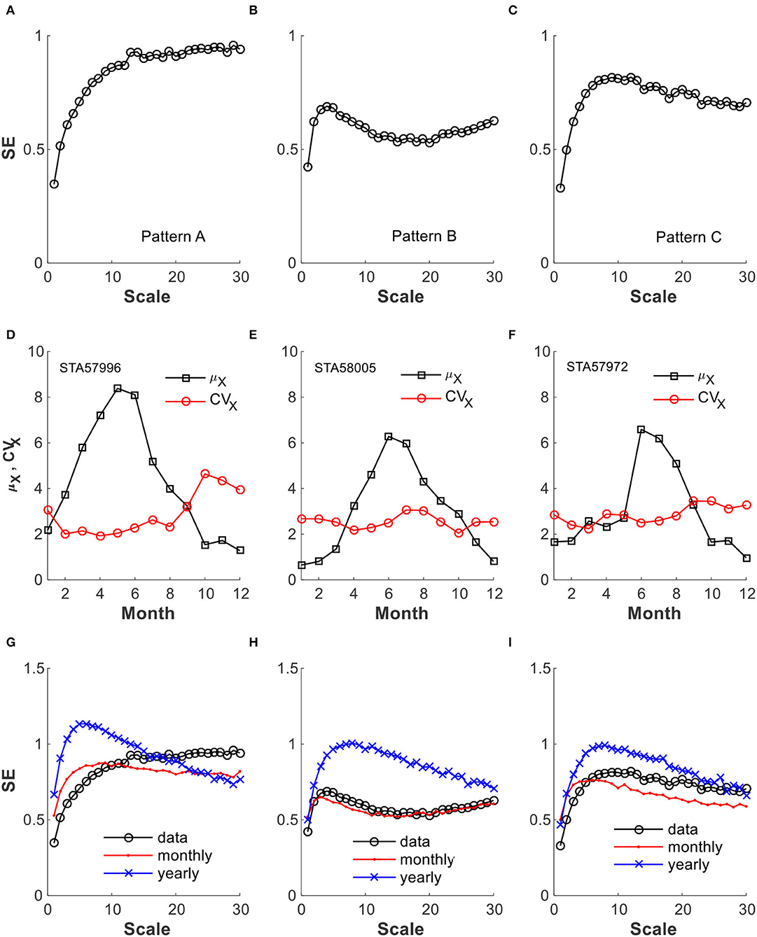
Figure 8. Typical MSE patterns and a comparison with those from simulated precipitation: (A–C) represent MSE patterns A, B, and C; (D–F) are the monthly μ_X and CV_X of the time series where these patterns were obtained; and (G–I) include MSE from time series generated in two different ways.

These three representative patterns plotted in Figure 8 are obtained on records from stations STA57996, STA58005, and STA 57972, respectively. It turns out that the preceding simulation results using gamma distribution summarized in Figure 7 are not good bases for interpreting the MSE from the actual records. First of all, all these three sets of data have CV_X lie within a narrow range, and according to Figure 7, they should all exhibit a similar MSE because of the narrow range of CV_X they encompass as discussed in the following: STA57996 record (Pattern A) has μ_X = 4.28 mm/day, CV_X=2.65; STA58005 record (Pattern B) has μ_X =2.98 mm/day, CV_X = 3.12; and STA57972 record (Pattern C) has μ_X = 2.95 mm/day, CV_X = 3.3. For this range of CV_X, from 2.65 to 3.3, the simulated gamma-distributed precipitation per Figure 7 would give Pattern C MSE. However, the results show that in comparison with the simulated results, Pattern A is similar to the one with high CV_X (e.g., CVX = 5 and CVX = 8) and exhibits a higher rate of change at small scales; Pattern C is similar to the one with low CV_X (e.g., CV_X = 3 or smaller), while Pattern B has no corresponding correspondence. It is clear that the precipitation characteristics as contained in the multiscale is not captured by a single gamma distribution fit of a long-term record.

A question thus arises: Why the simulated gamma-distributed time series do not capture MSE of real precipitation data? We think it is because the time series so generated do not contain the seasonal change information contained in the real precipitation record. The fact that the real data do show seasonal precipitation characteristics change is illustrated in Figures 8D–F, where the monthly μ_X and CV_X of each of the three records are computed by lumping monthly data together over all the recorded years. They clearly show that the precipitation undergoes changes between rainy seasons and dry seasons. To circumvent this drawback of simulating a precipitation time series based on a single gamma distribution function, we further generate simulated time series with monthly variation introduced.

Improved Simulated Time Series by Incorporating Seasonal Changes

To address the effects of the seasonal changes in precipitation, we simulate precipitation for each month of the year using its corresponding μ_X and CV_X of the base record and generate gamma-distributed daily precipitations for the number of days of that month. This is carried for each month of the year in the calendar order until the number of years targeted is reached. We denote the present procedure as “monthly” based, and the single gamma distribution as “yearly” based. Comparisons of MSE from these monthly-based simulated time series as well as those from the recorded data, denoted as “data,” are given in Figures 8G–I for Patterns A, B, and C, respectively. These monthly-based times series give MSEs that match reasonably well with those computed from the recorded data. The most dramatic improvement is for the case with Pattern B, in which the “monthly” simulated data resulted in an excellent MSE match with that from the “data,” while the “yearly” simulated data perform rather poorly. As for Pattern A, the trend is also preserved better with the “monthly” simulated precipitation, whereas for Pattern C both the “monthly” and the “yearly” simulated precipitation perform about the same with similar levels of deviation from the real records.

On further investigation, we found that the slight mismatch of MSE of “monthly” simulated data with real data (see Figure 8G) is due to the highly year-to-year variation of the precipitation of STA57996 record in the dry seasons from October to December. Figure 9A depicts the total number of days without rain for these 3 months over the 61 years of records. The data clearly show that there is high variability of dry days from year-to-year. In contrast, the simulated data using the same monthly distribution for each year give a small fluctuation as shown in Figure 9B. The overall statistics of the no-rain days in the dry season gives some indication of the differences observed here: The data give a mean of 71.4 days, with a standard deviation of 7.5 days, while the simulation gives a mean of 67.4 days and a standard deviation of 4 days. The data give about twice as much of the standard deviation. What this implies is that the year-to-year dry season characteristics, i.e., inter-annual variability, needs to be incorporated in studying the orderliness in the precipitation time series. Indeed, this is the case. A new simulation is thus carried out considering inter-annual variation of the precipitation in dry season, in which the precipitation of the 3 months of dry season is simulated using the monthly means and standard deviations for each individual month of each year, while the other months of the wet season still use the individual monthly distribution for all years without considering any inter-annual variability. Figure 10 demonstrates the improvement of such an undertaking. Specifically, without considering the year-to-year changes, the MSE starts to drop with scale, albeit slightly, after about the 6-day scale. However, by just considering the dry season's year-to-year (i.e., inter-annual) variability, the MSE so obtained agrees rather well with the raw data after initial phase.

FIGURE 9

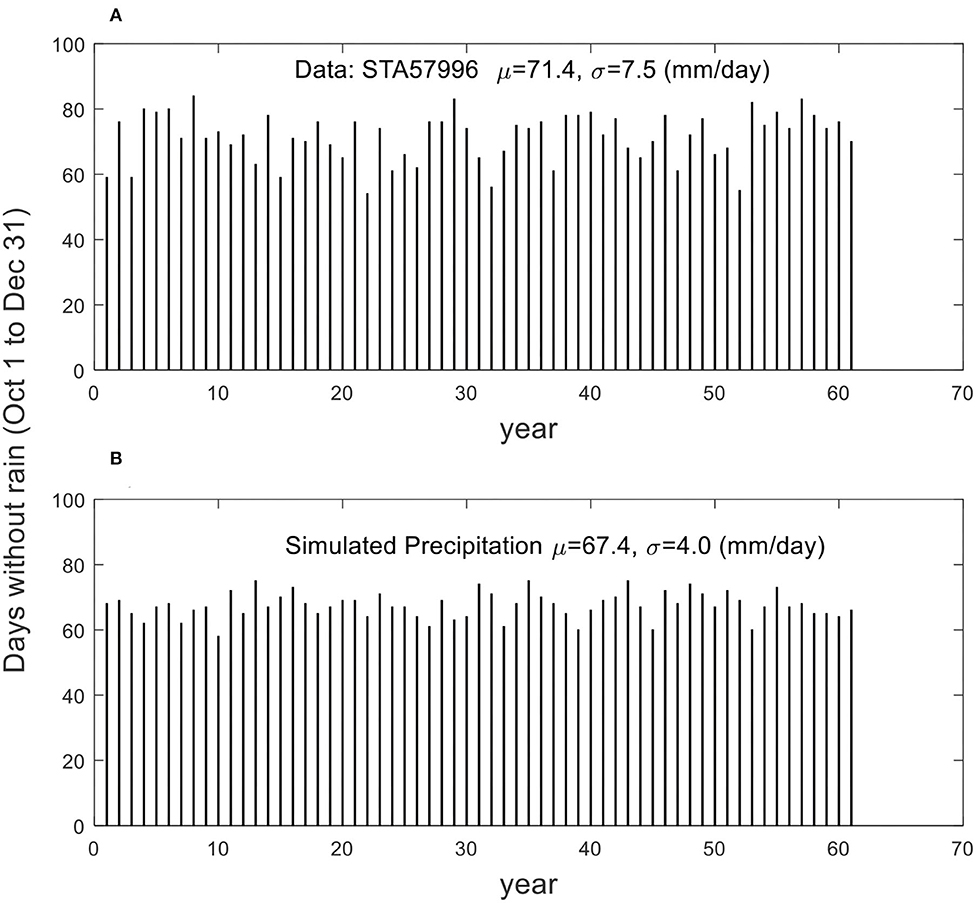
Figure 9. The days without rain of the dry seasons over 61 years (A) from STA57996 records, (B) from simulated data using monthly gamma distribution shown in Figure 8D.

FIGURE 10

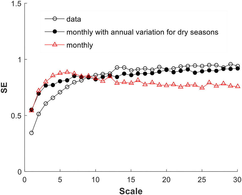
Figure 10. Real data MSE is better matched after introducing into simulation inter-annual variation of the precipitation in dry season.

Thus, it can be concluded that the MSE reveals the orderliness information in the precipitation that is not possible to grasp by simply fitting monthly or yearly probability distribution function to a time series without accounting for inter-annual variability, and the MSE could be valuable in guiding how simulated data should be generated. This is especially important for generating precipitation for a given designed level by considering non-stationary impacts due to climate change, as pointed out by researchers (e.g., Serinaldi and Kilsby, 2015; Serinaldi et al., 2018; Lawrence, 2020; Marra et al., 2020, and Slater et al., 2021).

Factors That Affect MSE Patterns

A further investigation of the MSE trend is conducted by varying the combination of monthly μ_x and CV_X. For this purpose, we define three climate patterns, they are, “wet,” “semi-arid,” and “arid.” For the wet climate, we consider it to have an annual precipitation of 1,470 mm, have two heavy rainy months, and that the precipitation increases gradually from dry season to reach its peak. The “semi-arid” climate is set to have less than half of the precipitation of its wet counterpart with annual precipitation reaching 621 mm. The “arid” climate is set to have relatively uniformly low precipitation throughout a year, and its rainy season is only slightly wetter resulting in an annual precipitation of 330 mm. The daily μ_x of each month in mm/day of these three climates is summarized in Table 1.

TABLE 1

Table 1. Monthly daily μ_x (mm/day) for different climates.

For further studying the impact of CV_X, we set out three scenarios as to how CV_X changes monthly (see Figure 11). Case 1 considers constant monthly CV_X of 3 (asterisk) for all three climates. Case 2 follows case 1 but increases in CV_X from 3 to 6 for dry months (square). As for case 3, it was set to reflect that the higher the precipitation, in general, the smaller the CV_X. As such, monthly daily CV_X is set inversely proportional to its monthly daily μ_x, and is scaled to lie between 1 and 6 (circular). A 61 years of simulated time series are generated for each scenario with inter-annual variability accounted, and as such the particular month in which a rainy season starts is irrelevant. The results obtained are summarized in Figure 11.

FIGURE 11

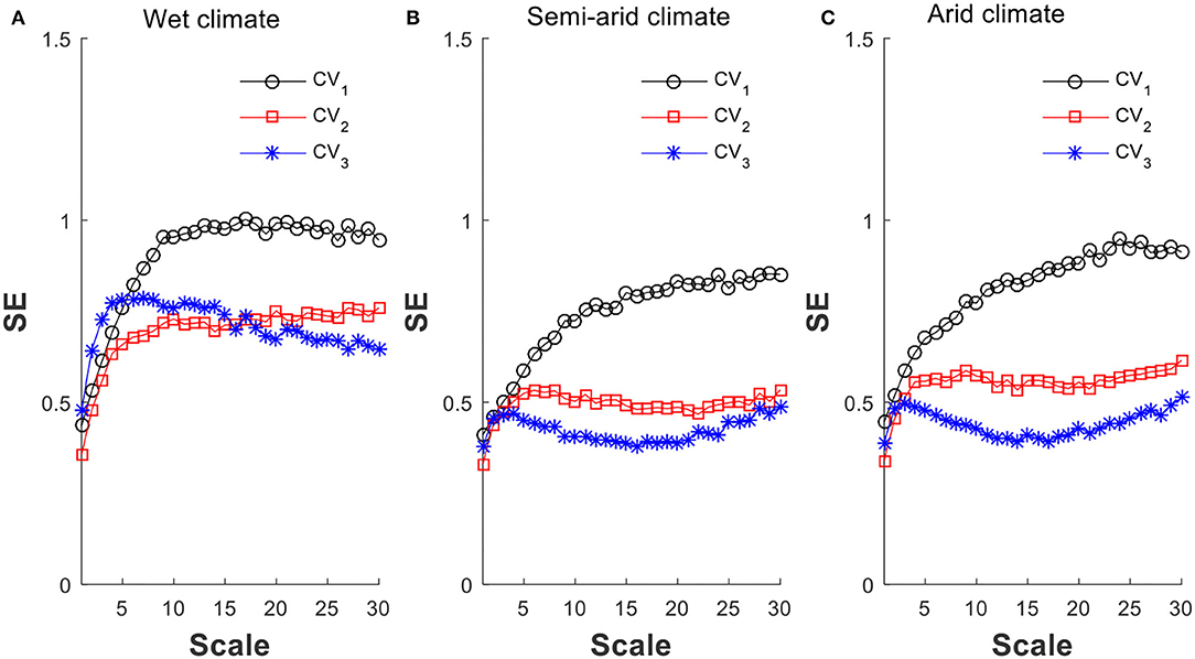
Figure 11. The shift of MSE patterns per the variation of μ_X and CV_X: (A) wet climate, (B) semi-arid climate, and (C) arid climate. Three cases of variation in daily CV_X: Case 1, asterisk, constant CV_X = 3; Case 2, square, CV_X = 6 for dry season and 3 for the rest; Case 3, circle, linear CV_X = 1 to 6, inversely proportional to monthly μ_X.

On examining the results as summarized in Figure 11, some observations can be made. For wet climate, Figure 11A shows that if CV_X stays constant (asterisk), i.e., case 1, the MSE follows Pattern C. However, as the CV_X is increased for dry season (square), i.e., case 2, the MSE moves toward Pattern A, and the larger contrast in CV_X per case 3 (circular) only increases the MSE in magnitude without altering its pattern. Figures 11B,C show that the semi-arid and arid climates give similar MSE trends. For cases 1 and 2, they exhibit Pattern B MSE, and for case 3, Pattern A. Neither case exhibits Pattern C MSE. These results also demonstrate that using strong contrast in CV_X as in case 3, the dry season precipitation variability is also amplified, and that is how it leads to Pattern A MSE. This is consistent with the observation made in the preceding section that additional variability is needed to produce Pattern A MSE when using monthly distribution in generating long-term precipitation time series.

Spatial Distribution of MSE Patterns

It turns out that the simple construct of Figure 11 explains the MSE patterns from the stations well. The MSE computed for each of the stations are presented in Figure 12 according to its location in the study area within China. It can readily be observed that the MSE of the same patterns appear in spatial clusters. To understand the underlying reasons of how these clusters are formed, the characteristics of the precipitation of the study region are examined. In addition to the annual precipitation over the study area presented in Figure 2, the spatial distributions of the monthly daily μ_x and CV_X are examined. For this, the drier winter months, i.e., from October to February, and the rest of the year, i.e., from March to September are plotted separately.

FIGURE 12

Figure 12. The spatial distribution of precipitation MSE patterns over the studied area (A) the spatial patterns; (B,C) are the daily μ_X and CV_X, respectively, from October to February; (D,E) are the daily μ_X and CV_X, respectively, for the period from March to September. Maps cover only the study area.

The stations with Pattern A MSE are located mainly in in the northwestern region and the areas close to the southern coastal region. The former includes the western Inner Magnolia as well as the southwestern and northern Tibetan Plateau. In the winter months, this northwestern region has μ_x mainly in the range of 0.01–0.66 mm/day and has the value of CV_X from 2 to >10. For the rest of the year, its μ_x values mainly vary between 0.05 and 2.67 with CV_X remaining highly variable to be in the range between 1.57 and 11.14. This reflects that the region is of arid climate, and with highly varying CV_X throughout the year. It is not surprising that the stations from this region exhibits primarily the Pattern A MSE. For the southern coastal region, in the winter months, it has μ_x in the range of 1.21–1.89 mm/day, while its CV_X value lies between 3.01 and 8. For the rest of the year, the southern region has μ_x between 4.11 and 10.83 mm/day, corresponding CV_X mainly ranging from 1.57 to 3.35. The high variation of CV_X from the winter months to other months, as demonstrated by Figure 11, is the reason why the precipitation of this region also exhibits Pattern A MSE.

The stations that exhibit Pattern B MSE dominate the studied area and span spatially from northeast toward southwest which covers the Northeastern region, North Plateau, Sichuan Basin, East and mid-east of Tibetan Plateau. Generally, these are semi-arid and semi-humid regions. The precipitation characteristics of these regions can also be roughly divided into two parts, an upper part and a lower part. The upper part of these regions has low winter precipitation, with μ_x in the range of 0.01–0.27 mm/day as denoted by the dark green dots in Figure 12B, with corresponding CV_X mainly lying within the range of 3–8. For the rest of the year, μ_x are in the range mostly between 1.31 and 2.67 mm/day with CV_X scattering within the range of 2.57–4.51. The lower part of the region is wetter as per the specifications given as follows: Its winter precipitation μ_x are in the range between 0.28 and 1.20 mm/day, and its CV_X lie in the range between 3 and 8. For the rest of the year, μ_x are in the range mostly between 1.31 and 5.68 mm/day and have CV_X scattering between 1.57 and 4.51. As Figures 11B,C demonstrate that for arid and semi-arid climates, when the variability in CV_X is not particularly high, the precipitation would exhibit Pattern B MSE. This not only explains the trend observed but also explains why it is the dominant pattern observed among all the stations studied.

The stations with Pattern C MSE are located in the middle and downstream regions of the Yangtze River. This region has very high winter precipitation, and the variability in the precipitation remains more or less constant all year round. Its μ_x mainly lie in the range of 1.90–5.55 mm/day, and its CV_X are in the range of 2.04–5. For the rest of the year, μ_x are in the range of 4.11–10.83 mm/day, and the corresponding CV_X are in the range of 1.57–3.35. The region is typical of wet climate with more or less uniform variability throughout the year, and as Figure 11A attests, the precipitation of the region exhibits Pattern C MSE.

It is clear that the spatial distribution of MSE patterns reflects the nature of precipitation in terms of monthly daily μ_x and CV_X distribution as discussed here. Moreover, not only that the MSE patterns for precipitation are similar for the stations that are close but also their magnitudes often lie within a narrow band. Figure 12 gives examples showing the similarity among the MSE patterns for the stations that are close; that is, the stations which are within 40 to 80 km distance apart. Such coherence over the distance may have important implication in water resource management planning.

Conclusions

MSE, through the introduction of scales and with the incorporation of similarity measures, shown in this study is capable of manifesting the changing complexity and it could serve as a useful tool for studying precipitation time series. This study has carried out basic groundwork in applying MSE to analyze complex precipitation time series. In this respect, we have confirmed the adequacy of using 2 for the dimensionality parameter, m, and 0.15 for the matching criterion, r. An equation is also presented for determining the required length, n, of the precipitation time series in terms of the desired scale. For obtaining the MSE up to a scale of 30-days, which is the case of this study, daily precipitation data of about 20,000-point long are needed.

The study has found that MSE can capture essential characteristics contained in a precipitation time series that are otherwise hard to detect. Above all, MSE is found sensitive to the interplay of the mean and CV_X, the seasonal cycle, and year-to-year changes (i.e., interannual variability) in arid climates. As a result, the MSE can be an effective tool for detecting differences associated with complex time series and for exploring factors affecting these differences. This capability is profoundly important especially with the gradual but continuously changing climates where the parameters (e.g., mean and standard deviation) associated with the underlying probability distributions are constantly changing. With the analysis framework presented in this study using the MSE, one can identify whether a stationary or a non-stationary time series would be a good candidate for the precipitation of the study region and how to best represent its non-stationary changing nature by adjusting the parameter values of its probability distribution. In our effort to generate the simulated precipitation time series, we also find that the MSE with those obtained from the actual recorded precipitation could serve as a powerful metric of evaluating the simulated results. It is shown that the conventional method, in which one distribution is used to generate a multi-year precipitation time series or even with one different distribution per calendar month is inadequate, because seasonal change can be important and such change may also have high interannual variability. We look into high interannual variability in dry season precipitation and find that MSE is able to discern the failure of a simulation procedure that incorporates different monthly gamma functions. We also find that such shortcomings can be amended by adopting different monthly gamma functions annually (i.e., considering interannual variability) for the dry seasons as illustrated by Figure 11. By making these changes, the two-parameter gamma distribution model is shown to work very well in terms of yielding the same MSE for the precipitation dataset studied.

Three main MSE patterns are identified based upon the precipitation data taken from 665 stations across China that have been continuously recorded for at least 50 years. In Pattern A, the SE increases with scale; in Pattern B, the SE increases initially with scale which after an interruption by a reduction continues to increase; and in Pattern C, the SE increases then reduces. Moreover, the spatial distribution of the MSE patterns over the studied area is found to reflect the spatial characteristics of precipitation. By partitioning the precipitation into dry winter season and the rest of the year, we found that the MSE patterns obtained can be interpreted properly. The MSE patterns also show coherence over distance in that stations that are close, which range 40–80 km, exhibit similar MSE trends. This could have important implications in using MSE for water resources management and planning.

Data Availability Statement

The original contributions presented in the study are included in the article, further inquiries can be directed to the corresponding author.

Author Contributions

XZ implemented the research ideas, processed all the precipitation data, performed the data simulation experiments, prepared most of the figures, and contributed to the manuscript writing at the beginning. J-SL and XL designed the simulation experiments, analyzed, and synthesized the results and co-wrote the manuscript. XL conceived the research ideas, supervised the investigation, and finalized the manuscript. All authors contributed to the discussions of the work. All authors approved the submitted version.

Conflict of Interest

The authors declare that the research was conducted in the absence of any commercial or financial relationships that could be construed as a potential conflict of interest.

Publisher's Note

All claims expressed in this article are solely those of the authors and do not necessarily represent those of their affiliated organizations, or those of the publisher, the editors and the reviewers. Any product that may be evaluated in this article, or claim that may be made by its manufacturer, is not guaranteed or endorsed by the publisher.

Acknowledgments

XZ would like to thank the China Scholarship Council for supporting his 2-year study at the University of Pittsburgh, and the partial support by the National Natural Science Foundation of China [Grant No. 51969006] and by the Science and Technology Funding of Guizhou Province [Grant Nos. (2019)2875 and (2018)5781-45]. XL would like to acknowledge the support from the William Kepler Whiteford Professorship from the University of Pittsburgh.

References

Amorocho, J., and Espidora, B. (1973). Entropy in the assessment of uncertainty in hydrologic systems and models. Water Resour. Res. 9, 1511–1522. doi: 10.1029/WR009i006p01511

CrossRef Full Text | Google Scholar

Avseth, P., Mukerji, T., and Mavko, G. (2005). Quantitative seismic interpretation. Episodes 3, 236–237. doi: 10.1017/CBO9780511600074

CrossRef Full Text | Google Scholar

Brunsell, N. A. (2010). A multiscale information theory approach to assess spatial-temporal variability of daily precipitation. J. Hydrol. 385, 165–172. doi: 10.1016/j.jhydrol.2010.02.016

CrossRef Full Text | Google Scholar

Burgueno, A., Martinez, M. D., Serra, C., and Lana, X. (2010). Statistical distributions of daily rainfall regime in Europe for the period 1951-2000. Theor. Appl. Climatol. 102, 213–226. doi: 10.1007/s00704-010-0251-5

CrossRef Full Text | Google Scholar

Chou, C. M. (2011). Wavelet-based multi-scale entropy analysis of complex rainfall time series. Entropy 13, 241–253. doi: 10.3390/e13010241

CrossRef Full Text | Google Scholar

Chou, C. M. (2012). Applying multiscale entropy to the complexity analysis of rainfall-runoff relationships. Entropy 14, 945–957. doi: 10.3390/e14050945

CrossRef Full Text | Google Scholar

Chou, C. M. (2014). Complexity analysis of rainfall and runoff time series based on sample entropy in different temporal scales. Stoch. Environ. Res. Risk. Assess. 28:1401–1408 doi: 10.1007/s00477-014-0859-6

CrossRef Full Text | Google Scholar

Costa, M., Goldberger, A. L., and Peng, C.-K. (2005). Multiscale entropy analysis of biological signals. Phy. Rev. E. 71, 021906. doi: 10.1103/PhysRevE.71.021906

PubMed Abstract | CrossRef Full Text | Google Scholar

Ebrahimi, N. (1999). Stochastic properties of a cumulative damage threshold crossing model. J. Appl. Probab. 36, 720–732. doi: 10.1239/jap/1032374629

CrossRef Full Text | Google Scholar

Ghosh, S. (2010). Modelling bivariate rainfall distribution and generating bivariate correlated rainfall data in neighbouring meteorological subdivisions using copula. Hydrol. Process 24, 3558–3567. doi: 10.1002/hyp.7785

CrossRef Full Text | Google Scholar

Hasan, M. M., and Dunn, P. K. (2011). Entropy consistency in rainfall distribution and potential water resource availability in Australia. J. Hydrol. Process. 25, 2613–2622. doi: 10.1002/hyp.8038

CrossRef Full Text | Google Scholar

Alves Xavier, S. F., Xavier, É. F. M., Jale, J. S., Stosic, T., and Santos, C. A. C. (2021). Multiscale entropy analysis of monthly rainfall time series in Paraíba, Brazil. Chaos, Solit. Fract. 151, 111296. doi: 10.1016/j.chaos.2021.111296

CrossRef Full Text | Google Scholar

Kawachi, T., Maruyama, T., and Singh, V. P. (2001). Rainfall entropy for delineation of water resources zones in Japan. J. Hydrol. 246, 36–34. doi: 10.1016/S0022-1694(01)00355-9

CrossRef Full Text | Google Scholar

Khan, M. I., Liu, D., Fu, Q., Azmat, M., Luo, M., Hu, Y., et al. (2016). Precipitation variability assessment of northeast China: Songhua River basin. J. Earth Syst. Sci. 125, 957–968. doi: 10.1007/s12040-016-0715-9

CrossRef Full Text | Google Scholar

Lake, D. E., Richman, J. S., Griffin, M. P., and Moorman, J. R. (2002). Sample entropy analysis of neonatal heart rate variability. Am. J. Physiol. Regul. Integr. Comp. Physiol. 283, R789–R797. doi: 10.1152/ajpregu.00069.2002

PubMed Abstract | CrossRef Full Text | Google Scholar

Lawrence, D. (2020). Uncertainty introduced by flood frequency analysis in projections for changes in flood magnitudes under a future climate in Norway. J. Hydrol. Reg. Stud. 28, 100675. doi: 10.1016/j.ejrh.2020.100675

CrossRef Full Text | Google Scholar

Li, X., Wei, N., and Wei, X. (2017). Complexity analysis of precipitation-runoff series based on a new parameter-optimization method of entropy. J. Hydrol. Eng. 22, 04017029. doi: 10.1061/(ASCE)HE.1943-5584.0001554

CrossRef Full Text | Google Scholar

Li, Z., and Zhang, Y. K. (2008). Multi-scale entropy analysis of Mississippi River flow. Stoch. Environ. Res. Risk Assess. 22, 507–512. doi: 10.1007/s00477-007-0161-y

CrossRef Full Text | Google Scholar

Liu, B., Chen, X., Lian, Y., and Wu, L. (2013). Entropy-based assessment and zoning of rainfall distribution. J. Hrdorl. 490, 32–40. doi: 10.1016/j.jhydrol.2013.03.020

CrossRef Full Text | Google Scholar

Liu, D., Cheng, C., Fu, Q., Zhang, Y., Hu, Y., Zhao, D., et al. (2018). Complexity measurement of precipitation series in urban areas based on particle swarm optimized multiscale entropy. Arab. J. Geosci. 11, 1–10. doi: 10.1007/s12517-018-3437-2

CrossRef Full Text | Google Scholar

Mangaraj, A. K., and Sahoo, L. N. (2010). A study on the probability distribution of daily rainfall amounts in western Orissa. Int. J. Agric. Stat. Sci. 6, 53–60.

Marra, F., Borga, M., and Morin, E. (2020). A unified framework for extreme subdaily precipitation frequency analyses based on ordinary events. Geophy. Res. Lett. 47, e2020GL090209. doi: 10.1029/2020GL090209

CrossRef Full Text | Google Scholar

Martinez-Villalobos, C., and Neelin, J. D. (2019). Why do precipitation intensities tend to follow Gamma distributins? J. Atmosp. Sci. 32, 3611–3631. doi: 10.1175/JAS-D-18-0343.1

CrossRef Full Text | Google Scholar

Maruyama, T., Kawachi, T., and Singh, V. P. (2005). Entropy-based assessment and clustering of potential water resources availability. J. Hydrol. 309, 104–113. doi: 10.1016/j.jhydrol.2004.11.020

CrossRef Full Text | Google Scholar

Mishra, A. K., Özgera, M., and Singh V, P. (2009). An entropy-based investigation into the variability of precipitation. J. Hydrol. 370, 139–154. doi: 10.1016/j.jhydrol.2009.03.006

CrossRef Full Text | Google Scholar

Pincus, S. M. (1991). Approximate entropy as a measure of system complexity. Proc. Natl. Acad. Sci. U.S.A. 88, 2297–2301. doi: 10.1073/pnas.88.6.2297

PubMed Abstract | CrossRef Full Text | Google Scholar

Quintero, F., Mantilla, R., Anderson, C., Claman, D., and Krajewski, W. (2018). Assessment of changes in flood frequency due to the effects of climate change: implications for engineering design. Hydrology 5, 19. doi: 10.3390/hydrology5010019

CrossRef Full Text | Google Scholar

Richman, J. S., and Moorman, J. R. (2000). Physiological time series analysis using approximate entropy and sample entropy. Am. J. Physil. 278, 2039–2049. doi: 10.1152/ajpheart.2000.278.6.H2039

PubMed Abstract | CrossRef Full Text | Google Scholar

Serinaldi, F., and Kilsby, C. G. (2015). Stationarity is undead: uncertainty dominates the distribution of extremes. Adv. Water Resourc. 77, 17–36. doi: 10.1016/j.advwatres.2014.12.013

CrossRef Full Text | Google Scholar

Serinaldi, F., Kilsby, C. G., and Federico Lombardo, F. (2018). Untenable nonstationarity: an assessment of the fitness for purpose of trend tests in hydrology. Adv. Water Resourc. 111, 132–155. doi: 10.1016/j.advwatres.2017.10.015

CrossRef Full Text | Google Scholar

Silva, D. F., Simonovic, S. P., Schardong, A., and Goldenfum, J. A. (2021). Introducing non-stationarity into the development of intensity-duration-frequency curves under a changing climate. Water. 13, 1008. doi: 10.3390/w13081008

CrossRef Full Text | Google Scholar

Singh, V. P. (1997). The use of entropy in hydrology and water resources. J. Hydrol. Process. 11, 587–626. doi: 10.1002/(SICI)1099-1085(199705)11:6<587::AID-HYP479>3.0.CO;2-P

CrossRef Full Text | Google Scholar

Slater, L. J., Anderson, B., Buechel, M., Dadson, S., Han, S., Harrigan, S., et al. (2021). Nonstationary weather and water extremes: a review of methods for their detection, attribution, and management. Hydrol. Earth Syst. Sci. 25, 3897–3935. doi: 10.5194/hess-25-3897-2021

CrossRef Full Text | Google Scholar

Xavier, S. F. A., da Silva Jale, J., Stosic, T., Costa dos Santos, C. A., and Singh, V. P. (2019). An application of sample entropy to precipitation in Paraíba State, Brazil. Theor. Appl. Climatol. 136, 429–440. doi: 10.1007/s00704-018-2496-3

CrossRef Full Text | Google Scholar

Zhang, L., Li, H., Liu, D., Fu, Q., Li, M., Faiz, M. A., et al. (2019). Identification and application of the most suitable entropy model for precipitation complexity measurement. Atmosph. Res. 221, 88–97. doi: 10.1016/j.atmosres.2019.02.002

CrossRef Full Text | Google Scholar

Zhang, L., Li, T., Liu, D., Fu, Q., Li, M., Faiz, M. A., et al. (2020). Spatial variability and possible cause analysis of regional precipitation complexity based on optimized sample entropy. Q. J. R. Meteorol. Soc. 146, 3384–3398. doi: 10.1002/qj.3851

CrossRef Full Text | Google Scholar