 Marwa Salayma
94% of researchers rate our articles as excellent or good
Learn more about the work of our research integrity team to safeguard the quality of each article we publish.
Find out more
ORIGINAL RESEARCH article
Front. Internet Things, 30 May 2024
Sec. Security, Privacy and Authentication
Volume 3 - 2024 | https://doi.org/10.3389/friot.2024.1306465
This article is part of the Research TopicSocio-technical Cybersecurity and Resilience in the Internet of ThingsView all 8 articles
This work presents a threat modelling approach to represent changes to the attack paths through an Internet of Things (IoT) environment when the environment changes dynamically, that is, when new devices are added or removed from the system or when whole sub-systems join or leave. The proposed approach investigates the propagation of threats using attack graphs, a popular attack modelling method. However, traditional attack-graph approaches have been applied in static environments that do not continuously change, such as enterprise networks, leading to static and usually very large attack graphs. In contrast, IoT environments are often characterised by dynamic change and interconnections; different topologies for different systems may interconnect with each other dynamically and outside the operator’s control. Such new interconnections lead to changes in the reachability amongst devices according to which their corresponding attack graphs change. This requires dynamic topology and attack graphs for threat and risk analysis. This article introduces an example scenario based on healthcare systems to motivate the work and illustrate the proposed approach. The proposed approach is implemented using a graph database management tool (GDBM), Neo4j, which is a popular tool for mapping, visualising, and querying the graphs of highly connected data. It is efficient in providing a rapid threat modelling mechanism, making it suitable for capturing security changes in the dynamic IoT environment. Our results show that our developed threat modelling approach copes with dynamic system changes that may occur in IoT environments and enables identifying attack paths, whilst allowing for system dynamics. The developed dynamic topology and attack graphs can cope with the changes in the IoT environment efficiently and rapidly by maintaining their associated graphs.
We live in a time where most aspects of life are becoming digital, relying on devices that connect with each other and to the Internet, leading to the so-called Internet of Things (IoT). Critical systems rely on the IoT, such as in healthcare (Saravanan et al., 2022; Sorri et al., 2022). It is assumed that control over the installation, integration, and usage of IoT devices lies with the user. In contrast to the traditional computers or cloud servers securely hosted in offices or contained within secure physical locations, IoT devices have dynamic aspects and are deployed in a physical environment that can be subjected to direct connections and both physical and cyberattacks. In many cases, systems are composed of several devices that join and leave a network dynamically or that may be intermittently connected. Such devices are often mobile, either because they are mobile themselves, such as autonomous vehicles or drones, or because they are instrumenting physically mobile objects, such as body sensor networks for healthcare. The diverse and advanced capabilities deployed by IoT devices, including the short-range communication protocols, enable IoT devices not only to interconnect with each other but also with other enterprise networks in the same environment, allowing a device or a whole network to join or leave other networks on-the-fly in an ad hoc manner (Agmon et al., 2019). When devices move location, they become exposed to new threats and cyberattacks that were not considered before, even if they had previously been thought to be secure.
Therefore, understanding how to maintain the operation of a system when it has been partially compromised is of critical importance. The key to achieving this is to find ways to enable a dynamic system to cope and respond to changes, which is a significant challenge and has not been addressed in the literature. Attack graphs are one way to model threats and propagation of attacks in an IoT environment. An attack graph is an attack modelling technique that depicts the attack paths followed by an attacker across the network to compromise a target, taking into account the vulnerabilities present in each device/host in the network and other reachable devices/hosts. Attack graphs show us the multistage of attacks and also help us decide on appropriate countermeasures to mitigate the effect of the system compromise (Jha et al., 2002). Legacy approaches of attack-graph modelling use static algorithms that do not adapt to changes in network devices and host configurations, their underlying topology, and/or security objectives (Noel et al., 2010). Calculating the attack graph when the system topology changes dynamically requires calculating the transitive closure, that is, reachability over the graph on the topology, to determine the reachable nodes. Although several algorithms exist to handle such changes in large graphs (Jin et al., 2012; Veloso et al., 2014), the problem does not have known solutions for dynamic graphs. Having gained privileges on a particular device, an attack can either exploit another vulnerability to elevate privileges on the same device or exploit a vulnerability on any other reachable host. It is, therefore, necessary to calculate the reachability to all other hosts from a particular one.
Interactive modelling and analysis of an attack graph are crucial to cope with changes in the network topology (we use topology as a synonym for a system), such as when a new device/host is added or removed from the system or when the configurations of host/devices change along with the network security objectives. The need for interactive modelling of rich and highly interconnected topologies, which are prone to continuous updates and are typically associated with large attack graphs, led us to consider the use of a graph database. A graph database models information by storing the data in nodes and connecting them through edges in a graph database, which is, as opposed to the relational database that is strict in terms of data modelling, more suitable to model, update, and query large, rich, and highly connected data. Hence, a graph database is an efficient methodology to model both the highly dynamic and interconnected topologies such as IoT networks and their large associated attack graphs (Barik and Mazumdar, 2014; Barik et al., 2016a).
Neo4j is a graph database management (GDBM) system that provides optimised and native graph storage and processing capabilities in which relationships attached to a node directly connect that node to other related nodes, allowing an easy way to traverse the graph and query graph paths and nodes. Neo4j adopts Cypher, a Neo4j built-in graph database query language that is specifically designed for graph-based reasoning. For example, Cypher can query graph paths traversing the graph without the need to use the index for joining data used in SQL relational database query language, which is slower than the graph database by many orders of magnitude (Chen et al., 2016). This is because the relational database requires expensive Cartesian products (join operations) with a complexity of O (nd) for traversing a graph of n nodes and of depth d (Noel et al., 2014). In Neo4j, however, one can traverse the graph through the direct edges that connect a node to other nodes, which means graph traversal complexity will depend only on the size of the resulted sub-graph and is not related to the total graph (Yuan et al., 2020). Using Cypher, one can query a graph database implemented in Neo4j to look for data matching a specific pattern. Neo4j has rich support for querying graph paths, allowing easy security analysis of attack graphs.
In addition to modelling the network topology graph existing in the environment using Neo4j, in this work, we have developed seven algorithms (implemented as Cypher queries) to investigate the propagation of attacks when the IoT environment changes using dynamic topology and attack graphs. These algorithms are developed to (i) generate the reachability graph automatically from a network-modelled topology graph, (ii) generate the attack graph from the reachability graph, (iii) merge two topology graphs when an existing network joins another one, which can be extended for multiple networks join each other, (iv) update the reachability graph only for the updated parts of the network, (v) merge two attack graphs when an existing network joins another one, (vi) de-merge the merged topology graphs when a network leaves, and (vii) de-merge the merged attack graphs when a network leaves. Furthermore, we developed queries to assess risk and attack propagation that allow us to re-evaluate the risk of compromise to different parts of the system when the environment changes.
This article is structured as follows: Section 2 discusses the few works in the literature related to the proposed approach to model threats in a dynamic IoT environment. We explain our proposed use case scenario drawn from healthcare systems in Section 3, followed by identifying and modelling our graphs, that is, the network topology, reachability, and attack graphs and their implementation using Neo4j in Section 4. The proposed approach for maintaining the dynamic graphs through the merging process is presented in Section 5; de-merging is presented in Section 6. We illustrate the application to our use case in Section 7 by running the queries for different scenarios related to our use case, while Section 8 shows how attack-graph-based metrics can be implemented to analyse the risk of compromise in the dynamic IoT environment. Finally, we discuss our conclusions in Section 9.
Different ways of representing attack graphs have been adopted in the literature. Attack graphs were first defined as a state-based approach where each node in the graph represents the state of the system (Swiler et al., 1998; Barik et al., 2016b). This approach was shown not to scale and is particularly unsuitable in IoT environments as every change to the network topology, such as adding a device, requires changing all the states in the model. In contrast, we adopt the so-called logical attack graph representation where nodes in the graph represent pre- and post-conditions and exploits that can be performed by the attacker leveraging known vulnerabilities (it is, in its strict sense, a bi-partite graph) (Jajodia et al., 2005; Jajodia and Noel, 2009). This formulation is also compatible with the application of Bayesian techniques as described in Muñoz-González et al. (2017) and also with a number of tools for attack-graph generation, such as Mulval (Ou et al., 2006). Pre- and post-conditions, in this case, correspond to expressions over the privileges required to exploit the vulnerability and privileges obtained after the vulnerability exploit, respectively. In their review article, Barik et al. (2016b) discuss the attack-graph generation and analysis techniques proposed in the literature. A more recent review on attack-graph generation is presented in Konsta et al. (2024), which discusses three methods for automatically generating both attack trees and attack graphs: model-driven, analysis-driven, and vulnerability-driven approaches. The review in Lagraa et al. (2024) addresses the advantages of using graph-based methods in network security and discusses a comprehensive quantitative and qualitative graph-based approach applied in network traffic analysis and botnet detection in particular. The survey also discusses the potential of using graph database tools in network security, such as Neo4j, and concludes that the benefits of using a graph database in network security applications are not well-harnessed yet. Several attempts that adopt attack graphs for risk and vulnerability assessment in IoT environments have been proposed in the literature. For instance, the work of Wang et al. (2018) uses an attack graph for vulnerability assessment in industrial IoT to achieve attack path finding and quantification. Although the proposed approach achieves a fast attack path finding and avoids repeat calculation, the work does not consider how the proposed approach performs in a dynamic IoT context. Almazrouei et al. (2023) discuss the state of the art of using attack graphs for vulnerability assessment in IoT networks and highlight modelling approaches for IoT vulnerability assessment, such as Markov decision processes and K-means clustering, in addition to other techniques that consider genetic algorithms, such as advanced reinforcement-learning algorithms. The survey emphasises that the dynamicity and continuous changes in the IoT typologies impose a main challenge in using the current attack graph methodologies for vulnerability assessment, which is the challenge that this article addresses.
Despite their usefulness in modelling and querying highly connected and scalable data, very few works have considered using GDBM systems to store and retrieve data related to network systems and/or attack propagation. However, information related to the network topology physical and logical components, the services installed on those components, the vulnerabilities of these services, the conditions to exploit the vulnerabilities, and the propagation of the attack are all data that can be stored and represented using graph database systems, one of which is Neo4j.
An early work that used Neo4j to model attack propagation in enterprise network topologies is presented in Barik and Mazumdar (2014). The work exploits dependency graph representation and assumes two types of nodes: entity nodes that represent the main component of an enterprise network, such as hosts, services, and their vulnerabilities, and fact nodes that represent interactions among entity nodes. However, the modelling of the network graph is troublesome due to the numerous types of fact nodes and edges between them, and many of the edges and nodes are not used or needed in the graph generation. This is because the work does not harness a feature of edge properties supported by Neo4j, which can help reduce the number of nodes and edges necessary to model the graph. The work assumes static reachability between hosts and between software services, whilst many details related to attack-graph generation, such as vulnerabilities, pre-, and post-conditions, are omitted. As a result, the generated attack graphs do not completely capture the full semantics of the network topology needed to analyse the attack paths, which leads to unrealistic graph modelling and query results.
Barik et al. (2016a) present an attempt to improve Barik and Mazumdar (2014) by introducing constraints that network topologies must enforce to represent the network access controls between machines necessary for the generation of the attack graphs. The work proposes a graph constraint language (GCON) as an extension over the standard property graph model, the model that Neo4j is built upon. The work adopts the exploit dependency graph representation. However, the constraint mechanisms are not clear, especially when it comes to the firewall rules queries and their impact on the reachability between hosts and their software services (firewall rules seem to allow traffic in both directions). As a result, the attack path was not a one-way directed path from the initial node to the target node, which makes it difficult to query and visualise the possible attack paths. Although information associated with vulnerabilities such as pre- and post-conditions is mentioned, they are not used in the attack-graph generation queries, and the work does not explicitly model the accessibility information between hosts in the attack-graph generation. As a result, the graph generation process is complex, especially when the network scales. How the firewall rules queries impact the reachability between hosts and how the reachability is calculated and queried are not clear in this work, which is similar to Barik and Mazumdar (2014).
Although they did not use Neo4j itself to generate the attack graph, Noel et al. (2014) used Neo4j Cypher queries to analyse an attack graph generated using the TVA/Cauldron tool. This tool was designed by George Mason University to generate and analyse attack graphs leveraging host vulnerability scans and firewall configurations, according to which it determines the reachability between machines in different domains. The work proposes a shared environment model with data ingested from other sources, such as the MongoDB database, and Apache Spark for network events, in addition to sources for network flows, IDS alerts, anti-virus logs, and so on. This shared environment is used as a database input to create a graph in Neo4j, which is then visualised, queried, and analysed to determine the security state of a network and how attackers can incrementally proceed with their attack. In Noel et al. (2016), the same authors developed an extended version of the shared environment—the CyGraph—to improve network security.
CyGraph leverages existing tools and data sources to build a knowledge graph. Similar to Noel et al. (2014), CyGraph uses the TVA/Cauldron tool to generate the attack graph for a network that considers firewall rules, host configurations, and vulnerabilities. CyGraph uses Neo4j to store the graph data (nodes, relationships, and properties) as its backend database. Graph pattern-matching queries are either expressed in Neo4j Cypher query language or using the domain-specific CyGraph Query Language (CyQL), complied by CyGraph to native Cypher. However, both Noel et al. (2014) and Noel et al. (2016) must import data from many sources to create the agnostic model. Some of those sources are commercial tools such as the Cauldron tool, which is used to generate the attack graphs, whilst Neo4j itself can be used to generate the attack graph associated with the network topology if it is provided with the means to consider the actual firewall rules and routing paths in the network. CyGraph is geared towards enterprise environments and does not consider IoT environments and their dynamic nature. Getting data from various data sources can be troublesome if the data related to network topologies are dynamic and continuously changing. CyGraph would need to update the data in all those input resources when the environment changes, making the proposed shared environment inconvenient for threat modelling in the dynamic IoT environment.
Yuan et al. (2020) use Neo4j to store information related to network machines along with their vulnerabilities. The work uses simple Cypher queries to investigate the directed attack paths initiated by exploiting a vulnerability in an initial node towards exploiting a vulnerability in the target machine. The attack graph is similar to those in Barik and Mazumdar (2014) and Barik et al. (2016a) and is generated over the topology graph. However, the way firewall rules are implemented, adding a node for each accessible port and adding edges between the nodes that can access each other, is not practical, especially if the network size or the firewall configurations change.
In all the studies discussed above, the graphs and queries implemented to generate or analyse the topology and the attack graphs consider static networks and do not account for what happens when the network environment changes; that is, new nodes are added or removed from the network or the network configurations and firewall rules change. Additionally, all the presented efforts that use Neo4j to generate the attack graph do so by creating an attack graph over the network graph itself ending in one graph, which makes it difficult to analyse and visualise both the topology and its associated attack graph or query them. This also makes it difficult to consider that multiple network graphs exist in the environment along with their corresponding attack graphs. Separate attack graphs and network topology graphs are required for this purpose and for better visualisation, investigation, query, and analysis. Most importantly, although few works considered traffic configuration polices, such as the firewall rules in their implemented static network topology, none of the work presented above shows how such packet filtering policies impact the reachability between hosts and how the attack graph is affected accordingly. How reachability between devices and hosts is calculated or how it changes when the environment changes is a major issue to consider when generating attack graphs in order to get sound query results.
In essence, reachable nodes in a graph mean there is a directed path between them, and this is typically computed by taking the transitive closure (the reachability matrix) of the graph computed, such as through the Floyd–Warshall algorithm, which states that there is a path between any two nodes in a graph if and only if there is an edge between the two nodes or there is a path between the two nodes going through any number of hops (nodes) (Weisstein, 2008). Xie et al. (2005) provided static modelling and representation for the reachability between routers in a TCP/IP network as a graph where the graph nodes represent the set of routers and the graph edges represent the connectivity between the routers. The work provided an attempt to compute reachability in a TCP/IP network that includes packet filters implemented in the routers to control the traffic between the routers. The work describes reachability between two routers as a subset of packets that the network will carry between the two routers, which can be computed using a set of union and intersection operations to reduce complex operations of computing the transitive closure. The work differentiates between instantaneous reachability in a network at a single instant in time, the upper bound reachability referring to the largest set of packets the network will ever deliver between two points, and the lower bound reachability referring to the largest set of packets the network will always deliver between two points. The work then provided approximations to the reachability bounds.
In this work, we are using Neo4j to query the reachability between devices/machines in our proposed topology graph by considering packet filtering rules implemented in routers. In contrast to Xie et al. (2005), our reachability queries can be considered instantaneous, assuming that the forwarding state is known at a specific instant, which requires knowing the configuration state of each router. However, not only can our reachability query run with a low time complexity, but it also can run only for the updated parts of the network whenever the network is updated or configuration changes by harnessing the Neo4j graph database features, as will be explained in Section 4.2.
As an example, we consider the scenario of a patient wearing a body sensor network (BSN), including sensors and a gateway (typically a mobile phone), visiting a clinic. This allows reasoning about the patient’s devices connecting to the clinic and thus acquiring reachability across the clinic’s system to other services and devices. For example, health apps on the patient’s device may need to connect to the services inside the clinic to upload monitoring data and download prescriptions for diagnostic tests or medication. The clinic may trigger re-calibration of the sensors on the patient. The important point to model is that the devices and services inside the clinic can become reachable from the patient’s devices and vice versa, thus creating new possible attack paths. Considering that the patient’s body sensor network comprises several devices and that the mobile phone acts as a routing gateway allows us to also consider the body sensor network as a ‘system’ and thus investigate what happens to the attack paths when systems become interconnected in a ‘systems-of-systems’ approach.
We have considered in detail the topologies of the two networks for the patient and for the clinic, as shown in Figure 1. For the clinic, we have considered different points of access to the network and access to a database and other network servers. We have also considered the internal segmentation of the clinic’s network in sub-networks, traffic filtering, and specific vulnerabilities on the devices drawn from NVD (Booth et al., 2013). Thus, we can model the attack paths originating from the patient’s devices that may lead to the database using attack graphs (Noel et al., 2010). We have also considered that the clinic has a connection to the Internet to consider the propagation of external attack paths across the combined systems. Similarly, we have considered vulnerabilities in the devices part of the patient’s body sensor network to consider attack paths from a clinic’s devices across the two systems that may lead to a target device on the patient (a Smartwatch). It is important to note that in contrast to the method adopted in the literature of generating an attack graph over the topology graph, we consider that the attack graphs for the two systems, that is, the patient’s BSN and the clinic, are computed independently and independent from their associated topology graphs. This approach allows us to consider merging and de-merging the attack graphs when topologies interconnect and dis-connect, in addition to allowing us to analyse the security characteristics of networks in the environment in a more efficient and easier manner.
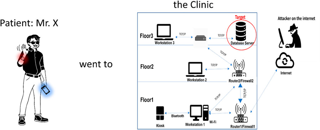
Figure 1. Example of our use case drawn from healthcare systems (patient and clinic).
Two types of attacks can be conducted in our patient–clinic use case scenario: (i) An external attack (the attacker is on the Internet) that attacks clinic systems remotely, and (ii) an internal attack that targets Bluetooth-enabled devices, and this attack is initiated internally while the attacker in close vicinity to any Bluetooth-enabled device, after which the attack can proceed remotely using the Internet. In this work, we are investigating the propagation of threats across both networks. To reason about that, we are considering different attackers with different targets: (1) one attack target, the Database Server, is located in the clinic topology, and the attacker attempts to get a root privilege over the Database Server; (2) the other attack target is located in the patient topology, the Smartwatch, to get a user privilege on the patient’s Smartwatch.
In our network topology, we have end devices such as IoT devices and workstations, as well as other network devices such as routers and switches. Each router can have different interfaces, allowing it to attach to different subnets. The routers are connected to each other, allowing communication between different routers associated with the different subnets. For example, in the clinic, all routers will be connected to Router1 (the aggregator), which connects the clinic to the Internet. Router 1 also has an interface that connects it to Subnet 1. We also have Router 2 that connects Subnet 1, Subnet 2, and Subnet 3 together, and Router 2 is connected to Router 1. Other routers can be created in the same way, and direct edges can be created between the routers and any end device if there is a direct physical connection between them. We consider that all routers can implement packet filtering rules that can deny access by default and only allow traffic flows that are explicitly allowed. End devices located in the same subnet are logically connected through the router. Hence, there is no direct edge between them. End devices that are not equipped with IP addresses can still communicate with each other, for example, through direct wireless links such as Bluetooth if they are within communication range. In such cases, we create a direct physical connection between the end devices to reflect this direct connectivity. This topology design leads to either direct connections between end devices and routers (or switches) or direct connections between end devices. All connection links between devices can also have additional attributes, such as the type of protocol that the connection allows (e.g., TCP, UDP, Bluetooth, and ZigBee). Without loss of generality, in our use case, we have only considered communication via TCP connections or direct communication via Bluetooth.
With this topology design and configuration, two assumptions for the possible routes populated in the routers’ routing table hold:
• Each router implements a routing table only for the routes associated with the networks to which the router is directly attached (directly connected). As a result, all the end devices, whether they are in the same subnet or in an adjacent subnet connected to the same router, can communicate with each other. In the latter case, they can communicate if and only if there is a firewall rule that allows the reachability between those two end devices, and this firewall rule can be implemented in the router that connects the different subnets directly.
• Each router in its routing table accounts for every single network in the network topology. This includes routes for the networks to which the router is directly attached (directly connected), as well as routes for the indirectly connected networks that can be either populated statically by the network administrator or shared dynamically between the adjacent routers through one of the networking protocols (Buchanan, 1999; Xie et al., 2005). For example, we can assume that each router in the clinic knows about the route for its directly connected subnets and the routes for indirectly connected subnets that are connected to the adjacent router and so on. As a result, the end devices in adjacent subnets connected to the same router or nonadjacent subnets connected through multi-hop routes can communicate with each other if and only if there is a firewall rule that allows the reachability between those two end devices and firewall rules are implemented in any router1.
In this work, we adopt the second assumption: that is, each router in its routing table accounts for every single network in the network topology through static or dynamic routing. As mentioned in Section 3, we have considered end-device vulnerabilities for both the clinic and the patient. In the clinic’s Floor 1/Subnet 1, Workstation 1 machine uses Windows OS and runs a vulnerable version of a web browser, which has CVE-2017-6753 vulnerability that allows an unauthenticated remote attacker to execute an arbitrary code and gain user privileges on that machine. Workstation 1 is also equipped with a Bluetooth adapter that has CVE-2017-8628 vulnerability in Microsoft’s implementation of the Bluetooth stack, allowing the attacker to obtain access to higher-level services and profiles and eventually obtain overall control. A kiosk end device is also located in the clinic on Floor 1; we assume it communicates and is managed directly by Workstation 1 through Bluetooth. The kiosk runs Linux OS and, like Workstation 2, has the Linux kernel stack overflow vulnerability CVE-2017-1000251 in its Bluetooth adapter. Workstation 2 in clinic Floor 2/Subnet 2 uses Linux OS and provides an FTP service that has CVE-2021-41635 vulnerability, allowing an attacker to abuse the machine configurations and obtain access to the entire machine. Workstation 2 is also equipped with a Bluetooth adapter, which has CVE-2017-1000251 vulnerability, that provides an attacker with a full and reliable kernel-level exploit for any Bluetooth-enabled device running Linux. Workstation 3 in clinic Floor 3/Subnet 3 also runs Linux and provides an SSH service with CVE-2022-30318 vulnerability, allowing an attacker to obtain overall control. The Database Server, also located in Floor 3/Subnet 3, runs Linux with kernel v.2.6 with MySQL RDBMS v.5, which has CVE-2009-2446 vulnerability that enables an attacker to gain user privileges on the Database Server.
For this example, we consider the Database Server as the end goal of an external attacker accessing from the Internet. The firewall implemented in Router 1 allows only HTTP traffic from the Internet to devices/machines in Subnet 1, that is, Workstation 1 and blocks all other traffic. The firewall implemented in Router 2 allows FTP and SSH traffic to Workstation 2 and to Workstation 3, respectively, as well as access to the Database Server from Workstation 2 and Workstation 3 and blocks all other traffic. The firewall rules for Firewall 1 and Firewall 2 are listed in Tables 1, 2, respectively.

Table 1. Firewall 1 rule set.
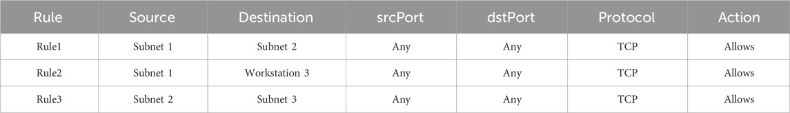
Table 2. Firewall 2 rule set.
For simplicity, we refer to the devices by their names rather than their IP addresses. Such topology examples, along with their physical components, packet filtering configurations, software vulnerability exploits, and associated pre- and post-conditions, which we will explain in detail in the following sections, are expected to provide an external attacker whose machine is on the Internet with two paths to access the target, the Database Server: either by exploiting the vulnerability in Workstation 1 from where the attacker can launch an attack on Workstation 2, which eventually leads the attacker to the database server, or the attacker can exploit the vulnerability in Workstation 3 from Workstation 1, which leads the attacker to exploit a vulnerability on the Database Server.
Our patient is wearing a Smartwatch that can connect to the patient’s Smartphone and any other Bluetooth-enabled device in its vicinity using a Bluetooth connection. The Smartwatch deploys sensors that sense critical physiological information, such as the patient's heart rate, making it a target for another attacker who wants to re-calibrate the sensors on the patient’s Smartwatch and manipulate the sensed data. The Smartwatch runs a Bluetooth stack in the Linux Kernel (BlueZ), which has CVE-2017-1000251 vulnerability, a stack overflow vulnerability that provides an attacker with a full and reliable kernel-level exploit. The patient also carries a Smartphone with an IP address that allows it to create a TCP/IP connection with any router around it. The Smartphone also has a Bluetooth connection, which allows it to connect with other Bluetooth devices in its vicinity. The patient’s Smartphone runs Android OS, which has a Bluetooth Android information leak CVE-2017-0785 vulnerability, allowing the attacker to access the whole phone filesystem, gain full control of a device, and use the victim’s Bluetooth interface to attack other devices in its proximity. In the following section, we show how we can model the network topologies of both the patient and the clinic.
We can model the network topology of any network using a graph GN = {V, E, A, C}, where V is the set of all the nodes in the graph, E is the set of all the edges in the graph, A is a set of attributes associated with nodes and edges, and C is a set of categories in which nodes and edges can be grouped. We discuss each of these graph elements in detail below.
• Graph nodes V = {Vd, Vv, Vr}, where Vd = {Ve, Vn} represents a set of all the devices in the network, which can be end devices Ve, such as IoT devices or workstations, or any other network devices Vn, such as routers and switches. Vv is the set of vulnerabilities that may exist in devices’ software services. Vr is a set of firewall rules implemented in the routers.
• Graph edges E = {Ed, Ev, Ef} where Ed is the set of all physical point-to-point connectivity links. This could be a direct connection between an end device and a router or switch (ve, vn), a direct connection between a router and a switch
• Attributes A = {Av, Ae} represent properties of the graph nodes and edges, where Av = {Ad, Avul, Ar} is a set of attributes that annotate the graph nodes representing the network devices, device vulnerabilities, and firewall rules, respectively. Ae, on the other hand, is a set of attributes that annotates the graph edges. For example, in our clinic topology graph, Ad = {name, Subnet, floor, accessibility, privilege}. Apart from the accessibility attribute, each of the attributes has a single value. An accessibility list ae is a set of features that allow an end device to access other devices. For example, Workstation 1 has an IP address and software services that allow access to other machines, such as the FTP and the SSH servers. Note that although there would typically be multiple user privileges on one device (e.g., for all the different users or for accounts with superuser privileges), for simplicity, in this work we assume that there is only one privilege on each device, either a user or a superuser privilege. Hence, the privilege attribute has a single value. Generally, we say ∀vd ∈ Vd ∃ad ∈ Ad. Another example, Avul = {preConditions, postConditions}, represents lists of pre-conditions required to exploit vulnerabilities and post-conditions that result from successful vulnerability exploits. Generally, we say ∀vv ∈ Vv ∃avul ∈ Avul. On the other hand Ae = {via} is the set of attributes that annotates the graph edges. The via attribute adds additional information about the connection between two devices, for example, specifying the protocol used, such as TCP/IP or Bluetooth. Attribute values, including the lists, are stored as strings.
• Categories C = {Cv, Ce} represent the sets of labels/types that help us filter the query results, where Cv is a set of labels that can be used to filter our query results for the graph nodes, such as by providing a name for the network topology graph to which the device belongs or by providing the type of the device whether it is an end device or a router or a switch and so on. Ce is used to filter query results for the edges. For example, it may indicate whether the edge represents a point-to-point connection between two devices
To create a node in the network, we must first specify its categories. For example, to create a node representing a device, we must specify to which network topology it belongs, the type of the device, that is, whether it is an end device or a network device, and to which subnet it belongs. In addition, we must specify its attributes: its name, which floor it is located in, and the accessibility features that allow it access other devices in the network, such as whether the device has an IP address and what other software services it supports (HTTP, FTP, SSH, MYSQL, and so on). The topology graphs for the systems in our use case scenario that refer to the clinic and the patient are represented in Figures 2, 3, respectively.
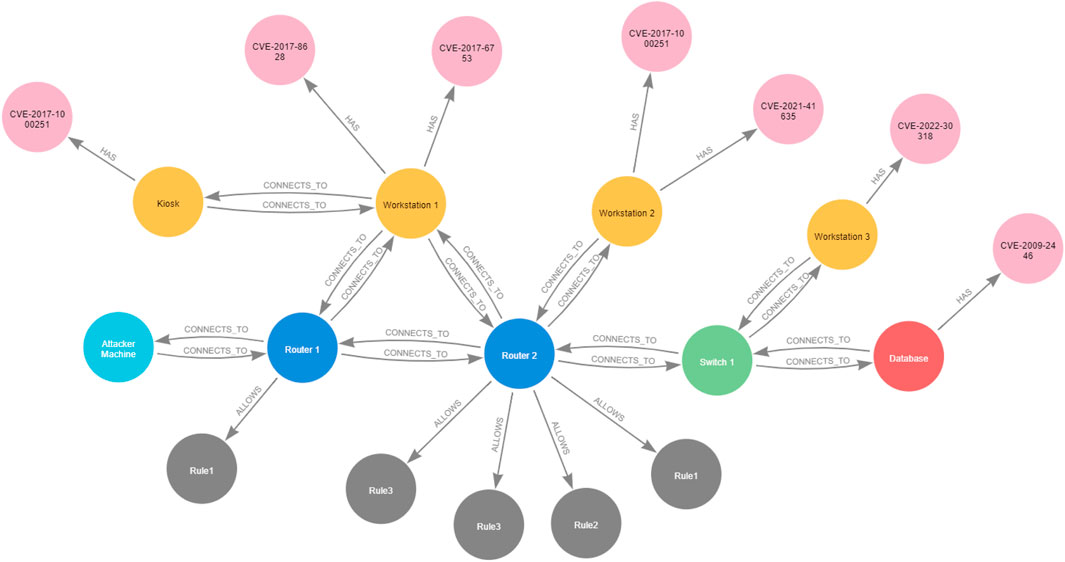
Figure 2. Clinic topology graph.
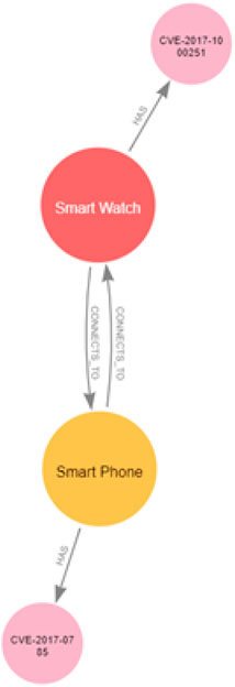
Figure 3. Patient topology graph.
The following are examples of how we are using Cypher queries to create nodes and edges in a graph to model the network topology of the clinic depicted in Figure 2.
Creating topology devices: we are referring to the clinic network topology graph
CREATE(n:ClinicTopology{name: ‘Workstation 1’, subnet: ‘Subnet 1’, floor: ‘floor 1’})
We can further specify that Workstation 1 is an end device by adding the appropriate category to Workstation 1 as follows:
MATCH(n:ClinicTopology) WHERE n.name= ‘Workstation 1’ SET n:EndDevice
In this way, we are adding the node n, which refers to Workstation 1, to the category/label cv = EndDevice, which also means that we are adding Workstation 1 to the set of end devices Ve in the set of devices Vd in
MATCH(n:ClinicTopology:EndDevice) WHERE n.name =‘Workstation 1’ SET n.accessibility =[‘IP’, ‘FTP’, ‘SSH’, ‘Bluetooth’]
Representing vulnerabilities in the graph: Workstation 1 is found to have two vulnerabilities. We can create a node representing one of those vulnerabilities as follows:
CREATE(v:ClinicTopology:Vulnerability {name:‘CVE-2017-8628’})
In the above query, we are adding the node v that we created to the set of vulnerabilities Vv that exist in the Workstation 1 software services by creating a new category called Vulnerability, and we set the name attribute of this vulnerability to CVE-2017-8628. A set of pre-conditions must be satisfied to exploit this vulnerability. Those conditions can be specified through the attribute preConditions associated with the vulnerability node. For example:
MATCH(v:ClinicTopology:Vulnerability {name:‘CVE-2017-8628}’}) SET v.preConditions =[‘User’,‘HTTP’]
By setting the attribute preConditions for the vulnerability node v, we represent that in order to exploit the vulnerability v, the attacker must be a user on the device from where they are launching the attack, and that device should support the HTTP protocol, that is, the attacker device should have the HTTP protocol in its accessibility list. A successful exploit of the vulnerability can lead to post-conditions, and those can also be specified through the vulnerability attribute postConditions. For example:
MATCH(v:ClinicTopology:Vulnerability {name:‘CVE-2017-8628’}) SET v.postConditions =[‘User’]
By setting the attribute postConditions for the vulnerability v, we state that after successfully exploiting the vulnerability v, the attacker will acquire the privileges of a user on the device that has vulnerability v. Then, in order to associate this vulnerability with Workstation 1, we can create an edge of type (category) ‘HAS’, which also means we are adding a new edge to the set Ev, as follows:
MATCH(n:ClinicTopology:EndDevice)
MATCH(v:Vulnerability)
WHERE n.name =‘Workstation1’ AND v.name =‘CVE-2017-8628’
CREATE(n)-[:HAS]->(v)
If we want to add a router to the topology graph, we can create a category/label called Router, to which we can add all routers that exist in the topology, which also means that we are adding a router with the name Router 1 to the set of network devices Vn in the set of devices Vd.
CREATE(r:ClinicTopology:Router{name:‘Router 1’}
Creating firewall rules: our firewall rules are implemented in the routers and control communication between devices in different subnets and with the Internet, and each router has its own firewall rules. Therefore, in order to write queries to state the firewall rules implemented in each router, we must first retrieve each router individually in addition to retrieving all devices in all subnets using the categories associated with them, as follows:
MATCH(i:ClinicTopology:Internet)
MATCH(s1:ClinicTopology:Subnet1)
MATCH(s2:ClinicTopology:Subnet2)
MATCH(s3:ClinicTopology:Subnet3)
MATCH(r1:ClinicTopology:Router{name:‘Router 1’})
MATCH(r2:ClinicTopology:Router{name:‘Router 2’})
We then can write the firewall rules listed in Tables 1, 2 using Cypher queries:
MERGE(f1:ClinicTopology:Firewall{name:‘Rule1’, source: i.name,
destination: s1.name, srcPort:‘any’, dstPort:‘any’, protocol:‘TCP’})
In the above query, we are making each rule in the rules set in a router firewall as a node belonging to the category Firewall with attributes corresponding to each item in the firewall tuples presented in Tables 1, 2 in Section 4.13. Rule 1 in the rule set of Firewall 1 states that any host on the Internet can communicate with any host in Subnet 1. Another way to do it is by creating rules associated with each end device in Subnet 1 one by one, but in this case, each rule requires a separate Cypher query. In this way, we are creating a node of variable f1 with a category called Firewall that will include all the firewall rules we have in the clinic topology, and we are adding f1 to the set of firewall rules Vr that are implemented in Router 1. Note that because there is only Workstation 1 in Subnet 1, one node representing the firewall rule will be generated, and if there are other end devices in Subnet 1, more than one firewall rule will be generated at the same time. The name of the firewall rule is Rule 1, and it addresses communication between devices located on the Internet and devices located in Subnet 1 in the clinic topology. As this rule allows devices on the Internet to reach devices in clinic Subnet 1, we create an edge of type ALLOWS that associates this firewall rule with the firewall implemented in Router 1, as follows:
MERGE(r1)-[:ALLOWS]->(f1)
Thus, we are presenting the action ALLOWS in each rule as an edge between the router that implements the firewall rule set, which also means we are adding a new edge to the set Er. We can do the same for the rest of the firewall rule sets and create directional edges of category ALLOWS between the routers and their rules. Although our network settings state that all traffic is denied by default, we can also implement less strict traffic restrictions by providing a mixture of both allows and denies rules. Similar to creating ALLOWS edges, we can easily add DENIES edges to our firewall rules queries. For example, we can explicitly state that the firewall implemented in Router 2 denies access between end devices in Subnet 1 and the database in Subnet 3 by adding the following Cypher query to the firewall rule set:
MERGE(f2:ClinicTopology:Firewall{name:‘Rule2’, source: s1.name, destination:‘Database’, srcPort:‘any’, dstPort:‘any’, protocol:‘TCP’})
MERGE(r2)-[:DENIES]->(f2)
Creating connection links (edges): we can see from the network topology in Figure 2 that Workstation 1 has a direct physical connection with Router 1. In the topology graph, we can represent this connection by creating bidirectional edges with category/type CONNECTS_TO between Workstation 1 and Router 1, as follows:
MATCH(n:ClinicTopology:EndDevice)
MATCH(m:ClinicTopology:Router)
WHERE n.name =‘Workstation 1’ AND m.name =‘Router 1’
CREATE(n)-[:CONNECTS_TO]->(m)
CREATE(n)<-[:CONNECTS_TO]-(m)
In this way, we are adding connectivity edges in both directions to the set of edges Ed that groups the physical point-to-point links between both Workstation 1 and Router 1. We can provide additional information related to these links by specifying an attribute that states the protocol used for this connection:
MATCH(n:ClinicTopology:EndDevice{name:‘Workstation1’})-[r]->
(m:ClinicTopology:Router{name:‘Router 1’}) SET r.via = ‘TCP’
The above query enables different types of CONNECTS_TO edges. For example, if the devices communicate through other protocols, such as the UDP, we can write the same query but setting r. via = ‘UDP’. Because several different protocols can be available over a connection, we can depict different types of traffic communication protocols by using different categories/types of connection edges, which eliminates the need to use the attribute via. For example, we can write the following Cypher query to create edges that represent a connection between two devices that exchange traffic through a TCP protocol:
MATCH(n:ClinicTopology:EndDevice)
MATCH(m:ClinicTopology:Router)
WHERE n.name= ‘Workstation 1’ AND m.name= ‘Router 1’
CREATE(n)-[:CONNECTS_VIA_TCP]->(m)
CREATE(n)<-[:CONNECTS_VIA_TCP]-(m)
We can write the following Cypher query to create edges that represent a connection between two devices that exchange traffic through the UDP protocol:
MATCH(n:ClinicTopology:EndDevice)
MATCH (m:ClinicTopology:Router)
WHERE n.name =‘Workstation 2’ AND m.name =‘Router 1’
CREATE(n)-[:CONNECTS_VIA_UDP]->(m)
CREATE(n)<-[:CONNECTS_VIA_UDP]-(m)
Without loss of generality, in our use case patient–clinic scenario, we are assuming one protocol for exchanging traffic between IP-enabled devices, which is the TCP protocol.
Firewall rules determine reachability between devices, and reachability is also controlled according to the construction of the routing table on each router. A router uses a specific network address to determine which out-link to use to reach a subnet. Conceptually, this is called a route. Hence, routing can be considered a kind of dynamic traffic filtering, which is why we are jointly considering traffic packet filtering and routing to determine reachability between end devices in our network topology graphs. As stated in Section 4.1, a router can infer about a route in multiple ways: (i) local routes that allow the router to reach all directly connected subnets, (ii) through static routes specified manually to map one or more router interfaces to a destination subnet, or (iii) routes shared dynamically between routers using a routing protocol, such as OSPF (Xie et al., 2005). Accordingly, two devices can reach each other if one or more of the following options apply:
• The two devices are in the same subnet.
• The two devices connect with each other directly, for example, through a short-range communication protocol such as Bluetooth.
• The two devices are indirectly connected through one or several routers (if they have IP addresses) if and only if the firewall rules allow. In this case, the devices can be in different subnets directly connected to a router or in different subnets connected to different routers that share the routes statically or manually.
After modelling our network topology using a graph, we can generate the reachability graph from the topology graph. This is described in the following section.
Let GR = {Ve, Er} represent our reachability graph. As is explained in Section 4.1.1, Ve represents the set of end devices, such as IoT devices or workstations, and Er describes the edges between end devices that are reachable from each other. A device can either have an IP address, which allows it to connect directly or indirectly with other devices in the network if the firewall rules allow, or it may not have an IP address if only direct communication is supported. However, not having an IP address will not hinder the end device from connecting and directly reaching other devices in the network using its unique MAC address or any other identifier, depending on the device’s communication technology. We can generate the reachability graph from the topology graph by considering that two end devices can reach each other if i) the two end devices are in the same subnet, ii) the two end devices have a direct point-to-point connection, or iii) the two end devices have an indirect connection. Hence, we can say that two end devices
Our reachability graph includes only the end devices from the topology graph and involves only one new category/type of edges Er, that is, REACHES. We say that nodes in a graph are reachable if there is a path between them, and this is typically computed by taking the transitive closure (the reachability matrix) of the graph, such as through the Floyd–Warshall algorithm, which states that there is a path between any two nodes in a graph if and only if there is a direct edge between them or there is a path between the two nodes going through any number of hops (nodes) between the two nodes (Weisstein, 2008). We can compute the reachability and generate the reachability graph between devices by using the Cypher query language in Neo4j.
Calculating the reachability from our network topology graph requires looking at the edges between end devices in our topology graph, as we assume our reachability graph includes only the end devices. Nevertheless, as explained in Section 4.2.1, one reason for reachability between end devices is that the two end devices are located in the same subnet. However, as long as we do not create and edge between nodes in one subnet in our topology modelling, we need only to check the subnet property of the two end devices in our network graph. Note that although the firewall rules presented in Table 1 and Table 2 explicitly state what devices can reach each other, we do not explicitly specify that devices in the same subnet can reach each other as they do so by default. This is why we must add this case as an individual case for reachability between end devices. Moreover, after running different experiments, we realised that considering nodes in the same subnet reach each other as an individual reachability case helps reduce the number of database hits4 as well the query response time compared to removing this case and adding the firewall rule to show explicit access between end devices in the same subnet.
Calculating the reachability for the rest of the cases presented above is very similar to the way we calculate the transitive closure following the Floyd–Warshall algorithm. As stated in Section 4.2.1, having a direct edge between two end devices means those devices are reachable through point-to-point connections, a case that can happen between IoT devices. Another case is that a path between two end devices through one hop can exist if the two end devices are connected directly to a router; that is, they are located in two different subnets to which a router is directly connected or connected indirectly through any number of routers (hops).
In Neo4j, a path between two nodes can be expressed using the asterisk (*). For example, (n)-[*2]- >(m) denotes exactly two relationships and one hop between nodes n and m. [*] without specifying bounds describes a path of at least one hop but of any positive length, that is, any/infinite number of hops, allowing us to query the existence of any indirect path between any two nodes. However, due to the firewall rules that constrain traffic flows, the existence of a path does not necessarily mean that those devices are reachable. It is also important to check that the firewall rules allow the respective traffic flows. Thus, finding the indirect path through the * should be accompanied by checking that a firewall exists in any router (by default, end devices are not allowed to communicate with each other unless explicitly stated otherwise by the firewall rules). Having said that, the reachability graph can be generated from our network topology graph using the following Cypher query:
MATCH(n:EndDevice)
MATCH(m:EndDevice)
WHERE n.name <> m.name AND (n.subnet=m.subnet
OR EXISTS((n)-[:CONNECTS_TO]->(m))
OR EXISTS((n)-[:CONNECTS_TO*{via:‘TCP’}]->(m))
AND EXISTS((:Router)-[:ALLOWS]->(:Firewall
{source:n.name, destination:m.name})))
MERGE(n)-[:REACHES]->(m)
The query above finds all the end devices in all the networks, and for any two different end devices n and m, creates an edge of category/type REACHES between them if any of the following conditions apply: 1. Two devices are in the same subnet; 2. The two devices are connected directly, for example, via a point-to-point link; 3. The two end devices are connected to each other indirectly (e.g., they can communicate through TCP/IP), and there is a firewall rule implemented in any router that allows communication between n and m. The * operator means that starting from node n and ending in node m, the graph is traversed to look for edges with the required protocol attributes, in this case via = ′TCP′. According to the reachability query results, we can add a new edge REACHES to the set Er. We can also add a query to check the existence of a path associated with a UDP protocol between any two devices; that is, we can add the following query to the above reachability query:
OR EXISTS((n)-[:CONNECTS_TO*{via:‘UDP’}]->(m))
However, if we created different types of CONNECTS_TO edges, for example, CONNECTS_VIA_TCP, CONNECTS_VIA_UDP, we can write the following query that allows us to traverse the graph for all types of edges associated with the traffic protocols we are interested in all at once. For example, we can add the following:
OR EXISTS((n)-[:CONNECTS_VIA_TCP | CONNECTS_VIA_UDP*]->(m))
The above reachability query allows us to generate the reachability graph between any two end devices across all the network topology graphs that exist in the environment at once, as we are not filtering the query to find end devices from a specific network graph or with a specific category (we can filter as we discussed in Section 1.1). However, this may slow the query outcome when the graph in the environment is large. For example, running the above reachability query for all the end devices in all the networks used in our use case requires 272 ms with 201,529 database hits in the Cypher query run time. Most of those hits lie in finding the path comprising CONNECTS_TO edges. We can limit the query by specifying which topology graph we are interested in. For example, we can query the clinic topology graph alone by providing the label ClinicTopology in the query as follows:
MATCH(n:ClinicTopology:EndDevice)
MATCH(m:ClinicTopology:EndDevice)
Focussing on the clinic topology alone, the query takes 191 ms, with 49,598 database hits. We conducted an additional experiment by gradually adding five more routers to the clinic topology, each with one subnet and one machine connected with each other over a chain of TCP connections. We ran the reachability query for the clinic and checked the query performance, which was almost the same in terms of the query running time and the number of database hits as the original clinic topology. By specifying the end devices in the patient topology alone, we achieved the query result in 300 ms, with 87 database hits, because the patient topology does not involve TCP connections. Although the pattern (n)-[*]- >(m) allows us to query paths between two nodes connected indirectly through several routers, the performance of a query involving this pattern could be reduced as the network size scales. We can harness filtering by specifying categories, and we can filter using appropriate attributes. For instance, one does not need to query the whole network graph to compute the reachability whenever the network changes, especially if the network administrators know where the update/change occurs, such as on a specific floor in the clinic. To find the reachability between end devices located on Floor 1 in the clinic topology, one can modify the first two lines of the reachability query by specifying the floor attribute:
MATCH(n:ClinicTopology:EndDevice{floor:’floor1’})
MATCH(m:ClinicTopology:EndDevice{floor:’floor1’})
By specifying that we wanted to find reachability for end devices located on Floor 1, we achieved the results in 10 ms, with only 204 database hits. We can also find the reachability between end devices located on different floors, for example, Floor 1 and Floor 3, by specifying the floors we are interested in as follows:
MATCH(n:ClinicTopology:EndDevice{floor:’floor1’})
MATCH(m:ClinicTopology:EndDevice{floor:’floor3’})
Our experiment to find the reachability between end devices located on Floor 1 and Floor 3 took only 6 ms to run and 369 database hits. This is a significant improvement in the reachability query performance compared to running the query for the whole network. In fact, the reachability query is the only query that traverses the graph searching for TCP connections as well as checking the firewall rules, making the processing time of the other queries used in this work negligible when compared to the reachability query, as the other queries require only checking directly connected nodes, and none try to find out paths with indirect nodes. If one wants to consider a mixture of ALLOWS and DENIES firewall rules, then one can run a reachability query that considers a firewall implemented in a router with a firewall rule that denies access between two end devices. To do so, the reachability query presented above can be easily amended by adding one more condition that checks whether a firewall connected to a router with an edge of category type DENIES exists, as follows:
MATCH(n:EndDevice)
MATCH(m:EndDevice)
WHERE n.name <> m.name AND (n.subnet=m.subnet
OR EXISTS((n)-[:CONNECTS_TO]->(m))
OR EXISTS((n)-[:CONNECTS_TO*{via:‘TCP’}]->(m))
AND EXISTS((:Router)-[:ALLOWS]->(:Firewall{source:n.name, destination:m.name})) AND NOT EXISTS((:Router)-[:DENIES]->(:Firewall {source:n.name,destination:m.name})))
MERGE(n)-[:REACHES]->(m)
The reachability graphs that correspond to the clinic and the patient topology graphs are represented in Figures 4, 5, which show the output that matches the reachability described through the firewall rules listed in Tables 1, 2.
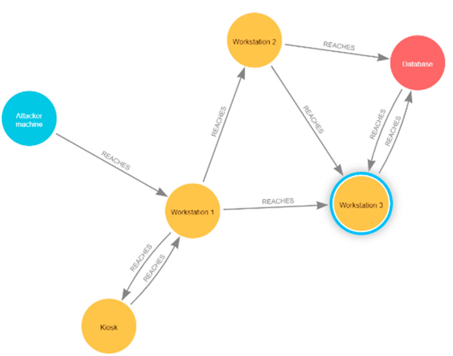
Figure 4. Clinic reachability graph.
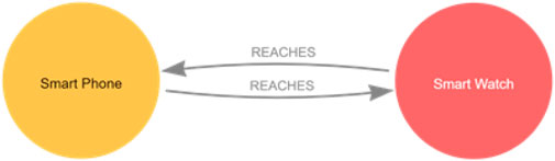
Figure 5. Patient reachability graph.
How an attack propagates in a certain topology can be modelled through an attack graph, which is a representation of all possible attack paths an attacker may follow to compromise critical resources. It uses the knowledge base of known vulnerabilities and attack techniques on a network and then finds the different sequences of exploits and attack paths starting from the attacker’s initial state, leading to the compromise of critical network assets (Agmon et al., 2019). To generate the attack graph for a system, in this instance, the clinic and the patient, it is necessary to first consider the topologies of the respective networks, which are represented in Figures 2, 3, respectively, in order to generate their associated reachability graphs. Next, from the reachability graph, we can generate the attack graph by considering the vulnerabilities present in each of the reachable devices, the pre-conditions necessary to exploit each vulnerability, and the privileges (i.e., post-conditions) obtained after the vulnerabilities are exploited. In short, we must know the following information to generate a network attack:
• The topology of the network.
• The devices in the topology.
• The vulnerabilities that may exist on those devices.
• The preconditions that must be satisfied in order to successfully exploit those vulnerabilities and whatever post-conditions result as an outcome of the successful vulnerability exploit.
• Traffic-limiting configurations, such as firewall rules that control the reachability between the devices in the topology.
As mentioned in Section 2, we adopt the exploit dependency graph representation (Barik et al., 2016b), and our approach to generating the attack graph for a specific network topology follows similar steps as those discussed in Barik et al. (2016a). However, in addition to all the information considered in Barik et al. (2016a) to generate an attack graph, in our work, we consider the information associated with vulnerabilities, such as pre- and post-conditions that are missing from Barik et al. (2016a), which only considers attacker gained privileges. In addition, we explicitly model the accessibility information between hosts in the attack-graph generation. Moreover, in contrast to the work in Barik et al. (2016a), which creates an attack graph merged with a topology graph in one graph, our approach must read information from the reachability graph and generate an attack graph separate from the topology and the reachability graphs, which makes it easier to query and analyse. Our attack graph can be defined as GA = (V, E), where V is the set of nodes in the attack graph and E is the set of edges that connect the nodes in GA. The attack graph involves two types of nodes, such that V = {Vc, Ve}, where Vc = {Vpre, Vpost} is a set of condition nodes that can either be pre-conditions required to exploit the device or post-conditions resulting from a successful exploit, whereas Ve is a set of vulnerability exploit nodes that represent an exploit of a vulnerability on software on a device. The attack graphs for the clinic and the patient are shown in Figures 6, 7 respectively. The pink nodes represent the conditions (either pre- or post-conditions), whilst the brown nodes represent vulnerability exploits.
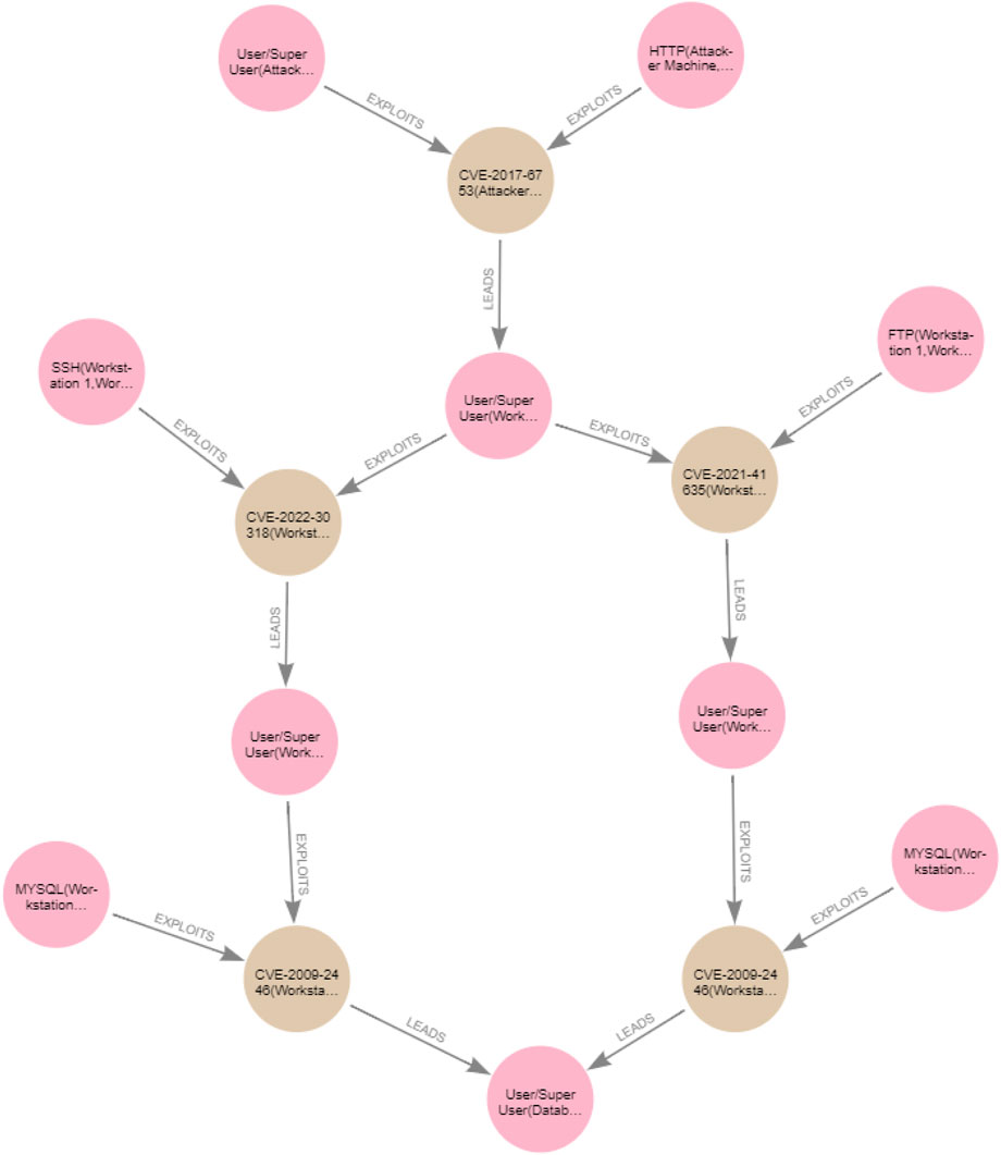
Figure 6. Clinic attack graph.
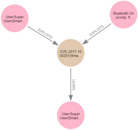
Figure 7. Patient attack graph.
Generally, in our attack graph, we say ∀vv ∈ Vv ∃vpr ∈ Vpre AND ∃vpo ∈ Vpost. Nodes representing pre- and post-conditions will be automatically generated when generating an attack graph. We assume that all the preconditions must be met to exploit a vulnerability. When it comes to vulnerability exploit nodes, any ve ∈ Ve has a name,
For example, to exploit the vulnerability CVE-2017-8628 in the Internet browser of Workstation 1, the attacker’s machine must use the HTTP protocol to connect to Workstation 1, which is a pre-condition required to successfully exploit CVE-2017-8628. If the attack is conducted successfully, then the attacker will become a user on Workstation 1, as this is the post-condition of the vulnerability. Hence, HTTP should be included in the attacker’s machine accessibility list, as well as in the pre-condition list associated with the CVE-2017-8628 vulnerability. Having user privileges on Workstation 1 is one pre-condition required to exploit the FTP vulnerability CVE-2021-41635 on Workstation 2, which is reachable from Workstation 1. The other pre-condition is that the attacker must use the FTP protocol to access Workstation 2; hence, Workstation 1 must support such protocol, that is, FTP should be included in the Workstation 1 accessibility list as well as in the pre-conditions list associated with vulnerability CVE-2021-41635. Only then can the CVE-2021-41635 vulnerability be exploited to give the attacker user privileges on Workstation 2 and proceed to the next vulnerability exploit.
Hence,
To generate the attack graph, we follow the steps presented in the pseudocode depicted in Listing 1:
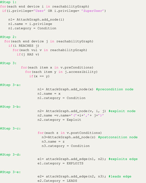
Listing 1: Attack-graph generation.
The following discusses each of the steps included in the pseudocode presented above:
1. For each device where the attacker has acquired user or super user privileges, create a condition node representing the privilege the attacker has gained on that device.
2. For each device reachable from the attacker device and which has one or more vulnerabilities,
3. And for each pre-condition in the pre-conditions list of each vulnerability in the reachable device, and for each item in the accessibility list of the device where the attacker acquired user/superuser privileges (i.e., the list of protocols according to which a device can initiate connections), check whether the pre-conditions to exploit each of those vulnerabilities are satisfied; that is, check the if there are accessibility features match the required pre-conditions to exploit each vulnerability, then
a. Create a condition node representing each of the satisfied pre-conditions that matches one or more of the attacker device accessibility features.
b. Create an exploit node representing the exploit of that vulnerability.
c. Create a condition node representing each item in the list of post-conditions associated with the vulnerability that represents the outcome of the successful attack on the device that has that vulnerability.
d. Create an EXPOLITS edge between the pre-condition node and the exploit node.
e. Create a LEADS edge between the exploit node and the post-condition node.
Using Neo4j, we have implemented Cypher queries that allow us to generate the attack graph from the reachability graph. Following the steps in the pseudocode in Listing 1, we can generate the attack graph for a network with a topology graph GN using Cypher queries. For example, for the clinic topology graph
Step 1:
MATCH(n:ClinicTopology:EndDevice) WHERE n.privilege =‘User(’+n.name+‘)’
OR n.privilege = ‘SuperUser(’+n.name+‘)’
MERGE(n1:Condition{name:‘User/SuperUser(’+n.name+‘)’})
ON CREATE SET n.targetTopology = ClinicTopology, n1:ClinicAttackGraph
Step 2:
MATCH(m:ClinicTopology:EndDevice)
MATCH(n)-[:REACHES]->(m)-[:HAS]->(v:Vulnerability)
Step 3:
UNWIND n.accessiblity as y WHERE ANY(x IN v.preConditions WHERE x = y)
Step 3-a:
UNWIND v.preConditions AS c
MERGE(n1:Condition{name:c+‘(’+n.name+‘,’+m.name+‘)’})
ON CREATE SET n1:ClinicAttackGraph
Step 3-b:
MERGE(n2:Exploit{name: v.name+‘(’+n.name+‘,’+m.name+‘)’})
ON CREATE SET n2:ClinicAttackGraph
Step 3-c:
UNWIND v.postConditions AS p
MERGE(n3:Condition{name:p})
ON CREATE SET n3:ClinicAttackGraph
Step 3-d:
MERGE(n1)-[:EXPLOITS]->(n2)
Step 3-e:
MERGE(n2)-[:LEADS]->(n3)
As expected in Section 4, the generated clinic attack graph reveals two attack paths that can lead the attacker to become a user/superuser on the Database Server. For example, to exploit the CVE-2009-2446 vulnerability on the Database Server from Workstation 2 that is, CVE-2009-2446(Workstation 2, Database), the attacker must be a user/superuser on Workstation 2 (user/superuser (Workstation 2)) and also access the Database Server through MYSQL from Workstation 2, that is, MYSQL (Workstation 2, Database). The successful exploit of CVE-2009-2446(Workstation 2, Database) leads to the attacker acquiring the user/superuser (database) privilege as a post-condition. The two attack paths in the clinic attack graph leading the attacker to become a user/superuser on the Database Server are
CVE-2017-6753(Attacker Machine, Workstation 1)->CVE-2021-41635
(Workstation 1, Workstation 2)->CVE-2009-2446(Workstation 2, Database)
CVE-2017-6753(Attacker Machine, Workstation 1)->CVE-2022-30318
(Workstation 1, Workstation 3)->CVE-2009-2446(Workstation 3, Database)
The generated patient attack graph reveals one attack path, leading the attacker to become a user/superuser on the patient Smartwatch, exploiting the vulnerability CVE-2017-1000251 from the Smartphone:
CVE-2017-1000251(Smartphone, Smartwatch)
If the attacker is a user/superuser on a device with accessibility features that allow it open connections and satisfy the pre-conditions required to successfully exploit a software vulnerability on a reachable device, allowing the attacker to eventually become user/superuser on the reachable device, then cycles may occur if the attacker device also has a vulnerability that requires pre-conditions to be exploited from the reachable device if that reachable device has accessibility features that allow it to open a connection with the attacker device. In other words, cycles in the attack graph may occur if the following condition applies: If there is an edge
To sum up, cycles will appear in the attack graph in this case: If
MATCH(m1:ClinicAttackGraph)-[]->(m2:ClinicAttackGraph)
cyclePath=shortestPath((m2)-[*]->(m1)) WITH m1
nodes(cyclePath) AS cycle WHERE m1:Exploit DETACH DELETE m1
As a result of running the above query, some conditions associated with the removed exploit nodes become isolated without edges. We can remove those remaining nodes (condition nodes) without edges, as having those isolated nodes, although not harmful, is useless. We can add the following Cypher queries to find those nodes with zero edges and delete them:
MATCH(n:ClinicAttackGraph)
WHERE SIZE—n)--())=0 DELETE (n)
In our attack graph, a cycle will be generated due to the exploit of the vulnerability of the Bluetooth adapter equipped in the Kiosk launched by an attack initiated from Workstation 1 and the exploit of the vulnerability of the Bluetooth adapter equipped in the Workstation 1 launched by an attack initiated from Kiosk. This is because both the Kiosk and the Workstation 1 are reachable from each other (when they are in the same Bluetooth vicinity), and the preconditions required to exploit the Bluetooth vulnerabilities in both of the devices are satisfied by each of them. However, as the attack target in the clinic topology is the Database Server, having this path (the cycle) from Workstation 1 to the Kiosk then to Workstation 1 is not useful in the clinic attack graph as this path will not lead the attacker to the Database Server, so we can remove this cycle from our attack graph as explained above.
When a sub-network joins another network, they may interconnect. As explained in Section 1, the topologies of both networks will be interconnected, and the reachability between the devices in both networks will change. As a result, their associated attack graphs will also be interconnected. Hence, we must do the following major steps to depict how attack propagation changes when two networks join each other and become interconnected:
1. Update (merge) the topologies of the involved networks, that is, create new connection links.
2. Re-generate the reachability graph of the merged topologies.
3. Re-generate the attack graph of the merged topologies.
The following sections describe each of these steps in detail.
In essence, if a device has an IP address, it will look for an access point (router device) with which a bidirectional TCP connection can be created (we only consider TCP traffic in our use case scenario) when it joins a new system. However, even if the device does not have an IP address, it still can create point-to-point links with devices in its vicinity. Hence, once a device joins a new system, different connectivity edges may be created. The outcome will be a merged topology comprising the original topologies of the networks we have in the environment, plus newly created CONNECTS_TO edges between them. In Neo4j, this can be implemented as follows:
MATCH(m1:EndDevice) WHERE ANY(x IN m1.accessibility WHERE x =‘IP’)
MATCH(m2:Router) WHERE NOT m1.targetTopology = m2.targetTopology
In the above query, we are looking for all the end devices that have IP addresses and all the routers we have in the environment. We are not filtering a specific network topology (through specifying a category); this is to ensure looking both ways between the two topology graphs in question, that is, the clinic and the patient, as the patient may also have routers. If those devices do not belong to the same network topology, then do the following:
MERGE(m1)-[:NEW_CONNECTS_TO {via:‘TCP’}]->(m2)
MERGE(m2)-[:NEW_CONNECTS_TO {via:‘TCP’}]->(m1)
SET m1:MergedTopologies, m2:MergedTopologies
In the above query, we are connecting the devices from the two network topologies with new TCP connections, that is, the edges of the new category/type of NEW_CONNECTS_TO. As we will discuss in the following section, this will distinguish the newly created links from the old links, which will help in finding the reachability only for the updated parts of the merged topologies. The above query allows us to find reachability for devices associated with new connections only and avoid re-calculating the reachability for the whole network. Thereafter, we add the devices associated with the newly created edges to a new category called MergedTopologies, which will help us merge and de-merge the associated attack graphs when the patient leaves the clinic or moves to a different floor. In addition to creating new connection edges via TCP, we are creating direct connection links due to the short comm protocols like Bluetooth. Such connection types require another condition to be satisfied: for example, the devices must be in the Bluetooth vicinity of each other. To achieve this, we write the following Cypher query:
MATCH(n1:PatientTopology) WHERE ANY(x IN n1.accessiblity
WHERE x=‘Bluetooth’)
MATCH(n2:ClinicTopology) WHERE ANY(x IN n2.accessiblity
WHERE x=‘Bluetooth’)
AND n2.floor = $floor
In the above query, we set the vicinity condition through the property floor, but we allow the user to specify the value of this property at run time through the parameter $floor to avoid needing to change the value of the floor manually each time the patient moves to a different floor. This is just one way of specifying the vicinity. In the above query, we consider only one example of short-range communication, Bluetooth, but this code can easily be upgraded for all possible short range communication technologies that allow different networks to merge with each other, considering any other condition required to create the connection edge. Next, we connect the Bluetooth-enabled devices from both networks using the following Cypher query:
MERGE(n1)-[:NEW_CONNECTS_TO{via:‘Bluetooth’}]->(n2)
MERGE(n2)-[:NEW_CONNECTS_TO{via:‘Bluetooth’}]->(n1) with n1, n2
n1:MergedTopologies, n2:MergedTopologies}
In fact, we can create new connections associated with different typologies that belong to other categories to merge with other networks. For example, imagine if another patient network topology with the category PatientTopology2 joins the clinic network. Then, as an example, we can create new connections associated with the second patient as follows:
MERGE(m1)-[:NEW2_CONNECTS_TO {via:‘TCP’}]->(m2)
MERGE(m2)-[:NEW2_CONNECTS_TO {via:‘TCP’}]->(m1)
SET m1:MergedTopologies, m2:MergedTopologies
We can do the same for multiple networks joining other networks each time we distinguish the new connections associated with the new merge using different edge categories/types. This guarantees only updating the reachability for the updated parts of the merged networks and avoids repeatedly querying all the networks to update the reachability results, as will be explained in detail in the following section.
Due to the newly created NEW_CONNECTS_TO edges in the merged network topology graphs, the reachability graph of both networks will inherently change. For example, new devices such as the the patient’s Smartphone are merged into the clinic topology and can reach other devices. Thus, we must re-generate an updated version of the reachability graph by running the following Cypher query.
MATCH(n:EndDevice)
MATCH(m:EndDevice)
WHERE n.name <> m.name AND (n.subnet=m.subnet
OR EXISTS((n)-[:NEW_CONNECTS_TO]->(m))
OR EXISTS((n)-[:NEW_CONNECTS_TO*{via: ‘TCP’}]->(m))
AND EXISTS((:Router)-[:ALLOWS]->(:Firewall {source: n.name, destination: m.name})))
MERGE(n)-[:REACHES]->(m)
Although the above query looks similar to the reachability query discussed in Section 4.2.1 that calculates the reachability for the whole network, the following query finds the reachability between the end devices associated with the newly created connection links in the merged topologies. Note that although the reachability query discussed in Section 4.2.1 can find the reachability in the merged topologies, using the query will repeat the work we have already done for the devices in their original network. That query already has poor performance and takes significant time and database hits due to the need to traverse the graph for all indirect TCP connections. Hence, we need a reachability query that can find reachability for only the updated parts of the networks in the merged topologies.
Note that the newly joined devices may or may not reach existing devices, depending on their connection modes and the firewall rules deployed, as explained in Section 4.1. In addition to checking the existence of the newly created links in the merged topologies, the above query still checks whether end devices belong to the same subnets, which is useful in case one adds a new device to a specific subnet in the current network, enabling the newly added device to reach and become reachable from devices in the same subnet. However, as in our merged topology query, we consider merging two networks by creating new connection links where necessary rather than adding a specific device to a specific subnet. We can omit the first case, which is checking whether devices belong to the same subnet when updating the reachability for the merged topologies. Instead, reachability between end devices in the same subnet can be assumed by default whenever one adds a new device to a specific subnet. The following query finds the reachability when a second patient joins the clinic network:
MATCH(n:EndDevice)
MATCH(m:EndDevice)
WHERE n.name <> m.name AND (EXISTS((n)-[:NEW2_CONNECTS_TO]->(m))
OR EXISTS((n)-[:NEW2_CONNECTS_TO* {via: ‘TCP’}]->(m))
AND EXISTS((:Router)-[:ALLOWS]->(:Firewall {source: n.name, destination: m.name})))
MERGE(n)-[:REACHES]->(m)
We tested our work for multiple patients joining the clinic, and our queries revealed the correct results. Due to space limitations, we will present the results of multiple networks joining and leaving each other in a future article.
When the reachability graph is updated, the attack graphs of both the clinic and the patient must be re-generated. Updating the attack graphs to represent the changes in the topology and the reachability graph requires re-running the query for generating the attack graph presented in Section 4.3.2 with two modifications: First, any newly generated node will be set to belong to a new category, the MergedAttackGraph (we can check that automatically using the MERGE clause)5. This is because during the merge of the attack graphs, new edges will be generated in the target attack graph, and new nodes will also be generated. For example, in the clinic attack graph presented in Section 4.3.2, we do not have any conditions or exploit nodes associated with vulnerabilities in the Kiosk software services. This is because the attack graph of the clinic is generated for attacks originating from the Internet. Involving attacking the Kiosk in the external attack would result in a cycle because the attacker would go to the Kiosk from Workstation 1 and back to Workstation 1 to proceed further to the database. Secondly, we must specify the target topology we are interested in in this work. Each network topology graph in the MergedTopologies category has its own target(s) and, thus, its own attack graph. For this purpose, we use a parameter (using $) allowing the user to specify the target they are interested in at run time instead of specifying statically as a hard-coded value. For example, Step 2 and Step 3-a in Section 4.3.2 would have the following minor modification:
Step 2:
MATCH(m:MergedTopologies:EndDevice)
WHERE m.targetTopology= $targetTopology
MATCH(n)-[:REACHES]->(m)-[:HAS]->(v:Vulnerability)
Step 3-a:
UNWIND v.preConditions AS c
MERGE(n1:Condition{name:c+‘(’+n.name+‘,’+m.name+‘)’})
ON CREATE SET n1:MergedcAttackGraphs
If we are interested in checking all the updates in all attack graphs associated with all merged topologies, then we must update (merge) the attack graphs associated with each network topology one by one in an iterative way. The target of interest must be specified each time.
In brief, when a system (sub-network) leaves, we must remove its nodes from the merged attack graph and remove all the edges that were added due to the interconnections between the two systems. In short, we must:
1. Update (de-merge) the merged topology graphs by removing the newly added connection links.
2. Update (de-merge) the merged attack graphs by removing newly added nodes and all edges associated with them.
These steps are explained in the following subsections.
As discussed in Section 5.3, in the merging process, new connection edges are added between the devices from the merged network topology graphs. REACHES edges are also created between devices in the merged topologies due to updating reachability for the updated part of the network. Hence, in the de-merging process, we only need to delete the new edges created between the merged topologies without removing the graph nodes representing the devices in the merged networks, which in our use case are the patient and the clinic networks. Moreover, we must remove those network components in the merged topology graphs from the MergedTopologies category. In other words, we can say:
MATCH(n1:PatientTopology)-[r]-(n2:ClinicTopology)
REMOVE n1:MergedTopologies, n2:MergedTopologies
DELETE r
The above query guarantees removing all the edges between end devices in the MergedTopologies category, whether they are NEW_CONNECTS_TO or REACHES edges. If there are multiple network topology graphs in the MergedTopologies category, we can filter which network topology graph we are interested in removing from the merged topologies. For example, if there are two patient topologies merged with the clinic network topology, and in the case that Patient 2 leaves the clinic while Patient 1 stays in the clinic, we can simply edit the above query as follows:
MATCH(n1:PatientTopology2)-[r]-(n2:ClinicTopology)
REMOVE n1:MergedTopologies, n2:MergedTopologies
DELETE r
The above query will remove the NEW2_CONNECTS_TO physical links as well as the REACHES edges associated with Patient 2 when their topology was merged with the clinic topology. This way, we can specify the category of the devices we are interested in removing and use filtering and categories to keep track of the nodes and edges added at each Merge operation. We tested our work for multiple patients joining the clinic, and our de-merge queries revealed the correct results. As mentioned previously, due to space limitations, we will present the description of multiple networks joining and leaving for a future article.
When the patient leaves the clinic, we must update the attack graphs by de-merging the attack graphs before merging them again if necessary; for example, if the patient moves to a different floor in the clinic. In de-merging the attack graphs, all we must do is find the nodes in the temporary category MergedAttackGraphs, which contains the newly added nodes that were not originally in the attack graphs, and delete them along with all the edges that connect them with the rest of the original nodes in the graph. This guarantees separating the original attack graphs corresponding to the network topology graphs and removing newly created nodes and all edges associated with them. In other words, we can say:
MATCH(n:MergedAttackGraphs) DETACH DELETE n
The above query guarantees de-merging all the merged attack graphs. If there is another merged attack graph in the MergedAttackGraph category associated with the Patient 2 topology graph in the MergedTopologies category, and if Patient 2 leaves, we must specify that in the MergedAttackGraphs category, as follows:
MATCH(n:PatientToplogy2:MergedAttackGraphs)
DETACH DELETE n
The above query guarantees de-merging only the attack graph of Patient 2 from all other merged attack graphs. Thanks to using categories (labels) to filter our queries, we can work only on the topology and attack graphs we are interested in.
To check the correctness of our algorithms and test whether their output aligns with expectations, we run the queries and show the output for merging and de-merging the graphs associated with the clinic-patient use case discussed in Section 3 when the patient enters the clinic’s Floor 1.6 We first run the experiments by considering that the target topology is the clinic topology, and then we run the same experiments considering the target topology is the patient topology.
The patient just entered the clinic and is now on Floor 1. Figure 8 depicts how the topology graphs of both the clinic and the patient merge on Floor 1, while Figure 9 depicts how the reachability graphs of both networks will be updated according to the merge. The figures show what is expected. As the patient’s Smartphone and Smartwatch are Bluetooth-enabled, they can reach all Bluetooth-enabled devices in their vicinity (Floor 1), in this case, the clinic’s Workstation 1 and the Kiosk. The patient’s Smartphone has an IP address. Once in the clinic, it will look for access points in the clinic to connect to, allowing the Smartphone to create TCP connections with Router 1 and Router 2. However, no firewall rule will allow the Smartphone to reach clinic end devices using TCP connections on any floor; hence, the Smartphone will only reach clinic Bluetooth-enabled end devices on Floor 1 through the Bluetooth short-range communication protocol. On the other hand, although Workstation 1 has an IP address, it cannot create TCP connections with any of the patient end devices because the patient does not carry or wear a router device.
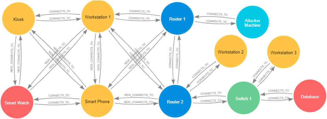
Figure 8. Merged topology graphs in the clinic on Floor 1.
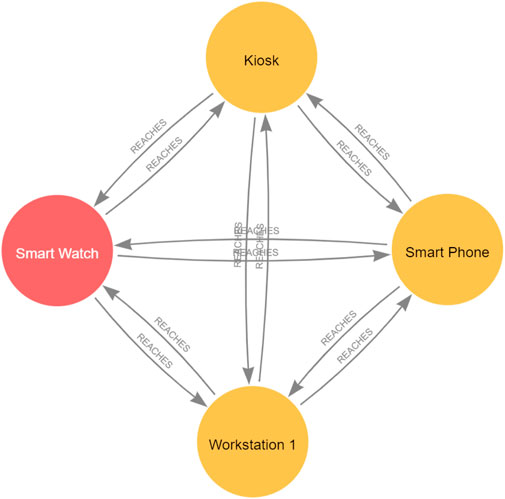
Figure 9. Updated reachability graphs in the clinic on Floor 1.
As a result, an internal attacker can exploit the Bluetooth vulnerabilities on both the Workstation 1 and the Kiosk from either the Smartphone or the Smartwatch because they satisfy the preconditions required to exploit those vulnerabilities on the clinic end devices located in Floor 1 (including the obtaining the required privileges), which is the assumed Bluetooth communication vicinity. The resulting merged attack graphs are shown in Figure 10.
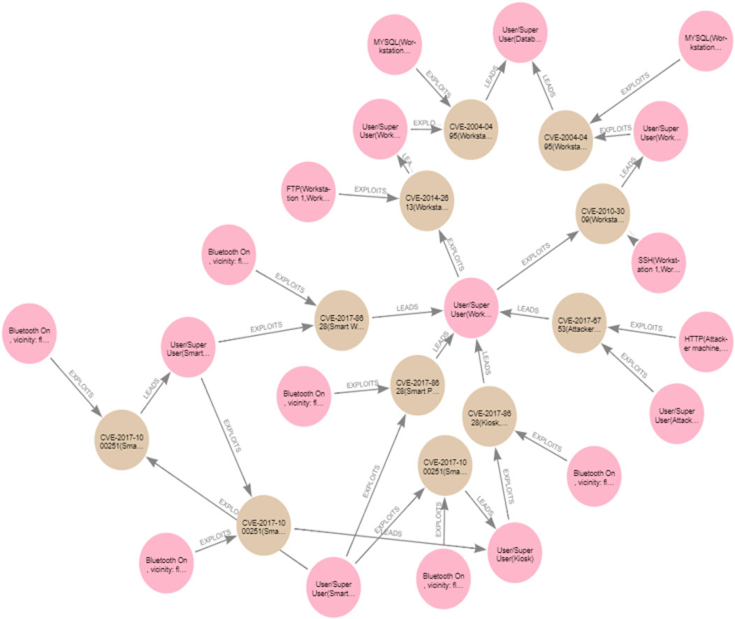
Figure 10. Merged attack graphs in the clinic on Floor 1.
Running the reachability query for the updated part of the network, as explained in Section 5.2, took 531 ms to run and required 1,681 database hits. This is a significant improvement, especially in terms of the total number of database hits compared to running the reachability query for the whole network, which will recalculate what has already been done. As our experiment in Section 4.2.1 revealed, running the reachability query for all the end devices in the network required 201,529 database hits. In contrast, the query for merging the topology graphs took 11 ms and required 616 database hits, while merging the attack graphs took 72 ms and required 4,681 database hits. As expected, the de-merge operations are very fast; they took 3 ms and 4 ms and required 93 and 38 database hits, respectively. The reachability query requires the longest time and the most database hits to be processed.
We continue our query testing as in Section 7.1, but we change the target topology to the patient topology. The merged topology and reachability graphs while the patient is on Floor 1 of the clinic should be similar to the ones in Figures 8, 9, respectively, which our experimental results revealed. The only difference will be in the merged attack graphs, as in this scenario, the directions of the directed attack paths are going towards the patient target, the Smartwatch, with the same number of attack paths (we will discuss how we can count the attack paths in Section 8), as shown in Figure 11.
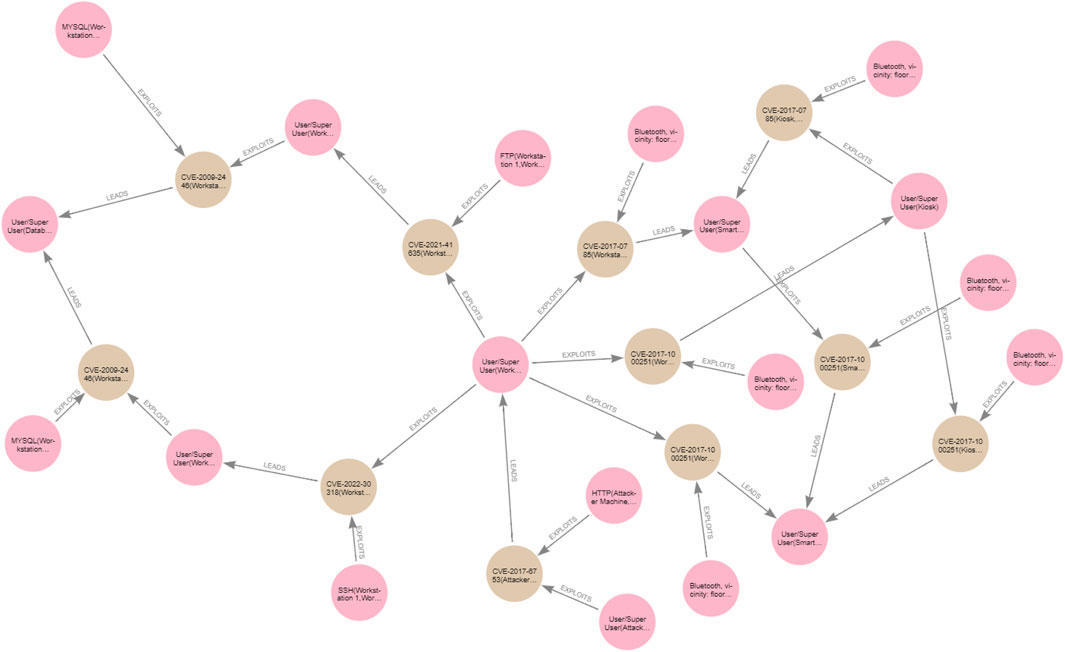
Figure 11. Merged attack graphs in the clinic on Floor 1, with the patient as a target topology.
As discussed in the previous sections, the attack graph is a modelling technique used to determine threats to critical system resources. Determining the possibilities of a cyberattack against critical resources, the potential impact of the attack on other parts of the system, and planning security countermeasures to prevent attacks on a system all fall under the umbrella of the concept of security risk assessment (Landoll, 2021). At its core, the attack graph provides a graphical security model to help assess the risk of attack on system components (Bopche and Mehtre, 2017). Our proposed method provides a means to assess risk and attack propagation that allows re-evaluating the risk of compromise to different parts of the system, as some parts of the system may have been compromised.
Usually, we assess the risk of attacks in a system against specific security metrics in order to identify and quantify security issues early enough so that we select appropriate countermeasures. Security metrics are used to assess the security of a given network configuration and to evaluate day-to-day changes in the security strength of a network (Bopche and Mehtre, 2017).
Several metrics for security risk assessment are summarised in Bopche and Mehtre (2017), such as the attack path length and non-path-length-based metrics, which were originally proposed in Phillips and Swiler (1998b), Ortalo et al. (1999), Li and Vaughn (2006), Lippmann et al. (2006), Pamula et al. (2006), and Idika and Bhargava (2010). In addition, a group of network hardening metrics were proposed by Noel and Jajodia (2014). The probability-based metrics proposed in Wang et al. (2007; 2008) are sensitive to the introduction of a new vulnerability in the network. The graph distance metrics discussed in Bopche and Mehtre (2017) determine changes in the network attack surface at a finer granularity and complement the traditional network monitoring approach for security risk mitigation.
In this section, we implement examples of Cypher queries for two attack-graph-based metrics, one of which is the shortest path metric (Phillips and Swiler, 1998b). The other represents the number of paths metric that was proposed in Ortalo et al. (1999).6
The shortest path metric represents the shortest distance from an attacker’s initial state to the attacker’s goal state (i.e., the target). In our attack graph, the shortest attack path means the path with the minimum number of edges (relationships) from the attacker’s starting point to the attacker's goal node (Phillips and Swiler, 1998a; Bopche and Mehtre, 2017). The category/type of nodes that can be included in the path is subject to the security expert performing the analysis. For example, we may want to involve the condition nodes, or we may want to count/view only the vulnerability exploit nodes along the path, or we may want to analyse both (Idika and Bhargava, 2010). In this work, we consider the number of conditions and exploits starting from the attacker’s initial state and proceeding in a chain to the attacker’s goal state. But how is this metric useful?
Intuitively speaking, from the perspective of the attacker, if there are multiple ways the attacker can follow to get to the target, the attacker will choose the path that requires the fewest steps. This relies on two assumptions: first, that the attacker is interested in using the minimum effort to reach the goal node, and second, that each step taken by an attacker includes a risk of being detected, so a minimum set of steps would, in principle, also minimise the attacker’s risk of being detected. Hence, the network with the shortest attack path is the network that is less secure, and the security engineer may prioritise patching the software vulnerabilities that exist along the shortest attack path.
However, although the shortest path attack metric can indicate the level of security of a network, this metric is not accurate in all cases. For example, as discussed in Ortalo et al. (1999), this metric alone does not indicate how many shortest paths exist in a network if more than one exists, which could lead to erroneous analysis and decisions. Moreover, this metric is not sensitive enough to be used for real-time network security evaluation independently: improving the security of the network by implementing countermeasures may result in a new attack graph for a more secure network, but the new network may have the same minimum path length as not implementing any countermeasure. Finally, the assumption that an attacker may choose the shortest path does not necessarily hold; attacker skill, for example, in exploiting a particular type of vulnerability or tooling, may induce different attack paths to be chosen. As a result, the shortest path metric can be too coarse (Idika and Bhargava, 2010).
Nevertheless, this metric can still effectively estimate how the security of the network might change when a new vulnerability is discovered or new countermeasures are being deployed.
Using the Neo4j Cypher language, we developed queries that identify, visualise, and measure the shortest attack path in a network. This metric can be applied and evaluated when the graph changes, such as when different systems are merged. For example, in our running example, the patient is on clinic Floor 1. The following query counts the shortest attack path and the length of that path between the patient's smartphone and the clinic Database Server when the patient is on clinic Floor 1. This path is depicted in Figure 12. We can do the same analysis for each network individually and for any other two nodes located in the same or different topologies and with multiple targets.

Figure 12. Shortest attack path between the patient’s Smartphone and the Database Server in the clinic, while the patient is on Floor 1.
MATCH(start:PatientTopology:EndDevice{name:’Smart Phone’})
MATCH(end:ClinicTopology:EndDevice {name:’Database’})
MATCH p = shortestPath((n:PatientAttackGraph:Condition{ name:’User/SuperUser(’+start.name+’)’})-[*]->(m:Condition:ClinicAttackGraph {name:’User/SuperUser(’+end.name+’)’}))
RETURN length(p)
OUTPUT: 6
The number of attack paths metric represents the number of ways an attacker can compromise a target in a given system and is an estimate of the network exposure to an attack (Phillips and Swiler, 1998a; Bopche and Mehtre, 2017). Intuitively, if the attacker has multiple ways to compromise a target node, the attacker has a better chance of achieving their goal without being detected. Hence, an attack graph with a larger number of paths is considered less secure.
This metric allows for the detection of fine granular changes in network security that the shortest attack path metric fails to detect. However, on its own, it may not give an accurate picture of the security of the network because the attacker's effort is not considered in this metric (Idika and Bhargava, 2010). For example, each path in a graph Ga of 10 attack paths could require 20 times more effort to violate than a graph Gb with one path, which means that Gb is less secure than Ga (Idika and Bhargava, 2010). However, there is no known way to quantify the required effort to propagate throughout the attack path in practice. For instance, the following query counts the total number of attack paths between the attacker's machine on the Internet and the target, that is, the database server in the clinic topology:
MATCH (start:ClinicTopology:EndDevice{name:‘Attacker Machine’})
MATCH(end:ClinicTopology:EndDevice{name:‘Database’})
MATCH path =(n:ClinicAttackGraph:Condition{name:‘User/SuperUser(’+start.name+‘)’})-[*]->
(m:ClinicAttackGraph:Condition{name:‘User/SuperUser(’+end.name+‘)’})
RETURN count(path)
Output: 2
Similar to the above, queries can be implemented to reason about attack paths and metrics in the patient attack graph. We can do the same analysis for each network individually and for any other two nodes located in the same or different topologies and with multiple targets. For example, the following query counts the number of attack paths between the patient’s Smartphone and the target in the clinic, that is, the Database Server when the patient is in the clinic Floor 1, and reveals there are eight attack paths between the Smartphone and the Database Server:
MATCH(start:PatientTopology:EndDevice{name:‘Smart Phone’})
MATCH(end:EndDevice:ClinicTopology{name:‘Database’})
MATCH path = (n:PatientAttackGraph:Condition{
name:‘User/SuperUser(’+start.name+‘)’})-[*]->
(m:Condition:ClinicAttackGraph{name:‘User/SuperUser(’+end.name+‘)’})
RETURN count(path)
Output: 8
The following Cypher query lists each of those eight attack paths along with its length:
MATCH(start:PatientTopology:EndDevice{name:’Smart Phone’})
MATCH(end:ClinicTopology:EndDevice {name:’Database’})
MATCH path = (n:PatientAttackGraph:Condition{ name:’User/SuperUser(’+start.name+’)’})-[*]->(m:Condition:ClinicAttackGraph
{name:’User/SuperUser(’+end.name+’)’})
RETURN count(p), length(p)
OUTPUT:
count(p) length(p)
2 6
4 8
2 10
We can run similar queries to check the total number of attack paths and the shortest attack path between the patient’s Smartwatch and the Database Server in the clinic. We can also do the same by changing the target topology to the patient topology and checking the total number of paths and the shortest path between any end device in the clinic and the patient target, that is, the Smartwatch.
This study has investigated the propagation of attacks in current and future IoT systems. In particular, an approach is developed to enable representing and maintaining attack paths through the system whilst allowing for system dynamics, considering not only the addition/removal of single devices but also the merging of graphs when multiple systems are connected and disconnected. This includes considering aspects of system topology and compositionality. Furthermore, the proposed method provides the means to assess risk and attack propagation that allows reevaluating the risk of compromise to different parts of the system.
We harnessed the efficiency of Neo4j, a popular graph-based tool, to map paths across the network. Neo4j allows us to model network and attack graphs, perform queries that provide quick results, and also allows for the filtering of large graphs and query subgraphs of interest, which saves search and query time complexities. For example, when the updates happen dynamically in the networks, our reachability query finds the paths associated only with the newly created links, that is, the updated part of the network, rather than querying all the paths, which would have a poor performance on a scalable network due to the need to traverse the graph for all indirect connections.
In comparison with previous reachability query approaches that query all paths with no consideration for avoiding duplicate calculations, we are not re-generating everything all the time. We showed the extent to which a graph database tool and the optimised implementation of queries on graphs make realising the solution to system dynamics and reachability problems in dynamic graphs possible by specifying exactly where and how to traverse certain parts of the network: using different edge types, filtering, categories, parameters, attributes, and so on. This optimised treatment of graphs allows parts of the system to be queried even before any updates take place or in static networks, as one does not need to query the whole network for reachability between all network components.
Our reachability query is the only query that requires traversing a graph searching for indirect connections between end devices. Compared to the other Cypher queries that we proposed, which all require only checking directly connected nodes, it takes the longest processing time and requires the highest number of database hits. In comparison, the processing times of the other queries proposed in this work are negligible. However, after running and testing our queries on different scenarios, results revealed that even when two systems are merged, running the reachability query on the merged graphs provided results in less than a second, with the number of database hits reduced significantly compared to running the query for the whole system. Our proposed network topology, reachability, and attack graph models can easily be extended by only creating new nodes, relationships, categories, and attributes; no changes to the database schema are required.
In addition to investigating the propagation of attacks in current and future IoT systems, we have developed queries to enable us to assess the risk of compromise in the dynamic IoT environment against security metrics evaluated on the graph of the different attack paths. As discussed earlier, the shortest attack path metric can be too coarse, while the number of attack paths offers a measure of the degree of flexibility the attacker has but does not necessarily capture an appropriate measure of risk to the system. It is, therefore, crucial to be able to analyse multiple metrics together because any single metric used in isolation may lead to a misleading analysis and conclusion about the risk to the system (Phillips and Swiler, 1998a; Bopche and Mehtre, 2017). Given that joining and leaving the network have a substantial impact on the properties of the attack paths, we have expanded our method to include other path-related risk assessment metrics. We discuss how we can use multiple metrics together, which are classified into decision metrics and assistive metrics. We have also enhanced the method to enable estimating the impact of compromise upon the functionality of the system. To achieve this, we have developed an approach using Neo4j and Cypher queries that enables us to analyse the interdependencies between system components. We modelled such interdependencies using a dependency graph, which also considers networked systems providing services whose functionality depends on other components in the network. This is because the availability of a given node is measured at the service level it provides as a proportion of the level normally expected of it. Fully estimating the risk and the impact of compromise when the environment changes enables us to select the most appropriate threat mitigation technique to deploy when the IoT environment changes based on its measured losses, impact, and costs over time. We are working on achieving this not only by using the methods implemented and/or related to this work, like the work in Soikkeli et al. (2019), but also through Bayesian inference according to a work previously done in Munoz-González and Lupu (2017). Due to the space limitation, we have not provided this part of the work in this article. We will discuss continuously analysing the risk and impact of compromise to build security control selection methods in an ongoing article that will be published soon.
The end goal we are seeking is the delivery of implemented tools and algorithms that can be either used independently for the analysis of more dynamic IoT scenarios or integrated into the broader tools of attack-graph analysis and risk evaluation developed to model threats in enterprise networks to enable them to deal with dynamic network scenarios.
The original contributions presented in the study are included in the article/Supplementary Material; further inquiries can be directed to the corresponding author.
MS: conceptualization, formal analysis, investigation, methodology, software, validation, visualization, writing–original draft, writing–review and editing, funding acquisition.
The author declares that financial support was received for the research and the authorship of this article. This work was supported by PETRAS National Centre of Excellence for IoT Systems Cybersecurity (PETRAS 2) under grant number EP/S035362/1. https://petras-iot.org/.
I thank Imperial College London for funding the article processing/publication through Imperial Open Access Fund.
The author declares that the research was conducted in the absence of any commercial or financial relationships that could be construed as a potential conflict of interest.
All claims expressed in this article are solely those of the authors and do not necessarily represent those of their affiliated organizations, or those of the publisher, the editors, and the reviewers. Any product that may be evaluated in this article, or claim that may be made by its manufacturer, is not guaranteed or endorsed by the publisher.
The Supplementary Material for this article can be found online at: https://www.frontiersin.org/articles/10.3389/friot.2024.1306465/full#supplementary-material
1The routers share their routes dynamically using routing protocols or statically (manually) by the network administrator; as a result, any end device in any subnet can reach any other end device in the clinic, even if it is not in the same subnet. However, reachability between devices can be limited by denying access between devices by default and using firewall rules to explicitly state which devices can communicate with each other.
2For simplicity, we are considering IP, a basic network protocol, as an accessibility feature in addition to the FTP and SSH, which are services that run on top of the IP and allow the device to access other devices’ software services. Some IoT devices do not have IP addresses to access other devices’ software services, so those devices will not include IP in their accessibility features.
3MERGE clause works like CREATE but only creates a node as specified in the query if that node does not exist already.
4A database hit is the abstract unit for retrieving or updating data to and from the storage engine requested by the Neo4j operators.
5When generating an attack graph, associated nodes will be created from scratch. When merging attack graphs, some nodes will already exist, and new ones will be created. We do not want to create nodes that are already there.
6We add extra examples in the Supplementary Material.
Agmon, N., Shabtai, A., and Puzis, R. (2019). “Deployment optimization of iot devices through attack graph analysis,” in Proceedings of the 12th conference on security and privacy in wireless and mobile networks, 192–202.
Almazrouei, O. S. M. B. H., Magalingam, P., Hasan, M. K., and Shanmugam, M. (2023). A review on attack graph analysis for iot vulnerability assessment: challenges, open issues, and future directions. IEEE Access 11, 44350–44376. doi:10.1109/access.2023.3272053
Barik, M. S., and Mazumdar, C. (2014). “A graph data model for attack graph generation and analysis,” in International conference on security in computer networks and distributed systems (Springer), 239–250.
Barik, M. S., Mazumdar, C., and Gupta, A. (2016a). “Network vulnerability analysis using a constrained graph data model,” in International conference on information systems security (Springer), 263–282.
Barik, M. S., Sengupta, A., and Mazumdar, C. (2016b). Attack graph generation and analysis techniques. Def. Sci. J. 66, 559. doi:10.14429/dsj.66.10795
Bopche, G. S., and Mehtre, B. M. (2017). Graph similarity metrics for assessing temporal changes in attack surface of dynamic networks. Comput. Secur. 64, 16–43. doi:10.1016/j.cose.2016.09.010
Buchanan, W. J. (1999). Networking fundamentals. London: Macmillan Education UK. doi:10.1007/978-1-349-14966-7
Chen, Y., et al. (2016). Comparison of graph databases and relational databases when handling large-scale social data. Saskatoon, SK: University of Saskatchewan. Ph.D. thesis.
Idika, N., and Bhargava, B. (2010). Extending attack graph-based security metrics and aggregating their application. IEEE Trans. dependable secure Comput. 9, 75–85. doi:10.1109/tdsc.2010.61
Jajodia, S., and Noel, S. (2009). “Topological vulnerability analysis: a powerful new approach for network attack prevention, detection, and response,” in Algorithms, architectures and information systems security (World Scientific), 285–305.
Jajodia, S., Noel, S., and O’berry, B. (2005). “Topological analysis of network attack vulnerability,” in Managing cyber threats (Springer), 247–266.
Jha, S., Sheyner, O., and Wing, J. (2002). “Two formal analyses of attack graphs,” in Proceedings 15th IEEE computer security foundations workshop, 49–63. CSFW-15. doi:10.1109/CSFW.2002.1021806
Jin, R., Ruan, N., Dey, S., and Xu, J. Y. (2012). “Scarab: scaling reachability computation on large graphs,” in Proceedings of the 2012 ACM SIGMOD international conference on management of data, 169–180.
Konsta, A.-M., Lafuente, A. L., Spiga, B., and Dragoni, N. (2024). Survey: automatic generation of attack trees and attack graphs. Comput. Secur. 137, 103602. doi:10.1016/j.cose.2023.103602
Lagraa, S., Husák, M., Seba, H., Vuppala, S., State, R., and Ouedraogo, M. (2024). A review on graph-based approaches for network security monitoring and botnet detection. Int. J. Inf. Secur. 23, 119–140. doi:10.1007/s10207-023-00742-7
Landoll, D. (2021). The security risk assessment handbook: a complete guide for performing security risk assessments. Boca Raton: CRC Press.
Li, W., and Vaughn, R. B. (2006). “Cluster security research involving the modeling of network exploitations using exploitation graphs,” in Sixth IEEE international symposium on cluster computing and the grid (CCGRID’06) (IEEE), 26.
Lippmann, R., Ingols, K., Scott, C., Piwowarski, K., Kratkiewicz, K., Artz, M., et al. (2006). “Validating and restoring defense in depth using attack graphs,” in MILCOM 2006-2006 IEEE military communications conference (IEEE), 1–10.
Munoz-González, L., and Lupu, E. C. (2017). “Bayesian attack graphs for security risk assessment,” in ST-153/RWS-21 NATO workshop on cyber resilience, 64–77.
Muñoz-González, L., Sgandurra, D., Barrère, M., and Lupu, E. C. (2017). Exact inference techniques for the analysis of bayesian attack graphs. IEEE Trans. Dependable Secure Comput. 16, 231–244. doi:10.1109/tdsc.2016.2627033
Noel, S., Harley, E., Tam, K. H., and Gyor, G. (2014). Big-data architecture for cyber attack graphs. MITRE case.
Noel, S., Harley, E. T., Tam, K. H., Limiero, M., and Share, M. E. (2016). Chapter 4 – cygraph: graph-based analytics and visualization for cybersecurity. Handb. Statistics 35, 117–167.
Noel, S., and Jajodia, S. (2014). “Metrics suite for network attack graph analytics,” in Proceedings of the 9th annual cyber and information security research conference, 5–8.
Noel, S., Wang, L., Singhal, A., and Jajodia, S. (2010). Measuring security risk of networks using attack graphs. Int. J. Next-Generation Comput., 113–123.
Ortalo, R., Deswarte, Y., and Kaâniche, M. (1999). Experimenting with quantitative evaluation tools for monitoring operational security. IEEE Trans. Softw. Eng. 25, 633–650. doi:10.1109/32.815323
Ou, X., Boyer, W. F., and McQueen, M. A. (2006). “A scalable approach to attack graph generation,” in Proceedings of the 13th ACM conference on Computer and communications security, 336–345.
Pamula, J., Jajodia, S., Ammann, P., and Swarup, V. (2006). “A weakest-adversary security metric for network configuration security analysis,” in Proceedings of the 2nd ACM workshop on Quality of protection, 31–38.
Phillips, C., and Swiler, L. P. (1998a). “A graph-based system for network-vulnerability analysis,” in Proceedings of the 1998 workshop on New security paradigms, 71–79.
Phillips, C., and Swiler, L. P. (1998b). “A graph-based system for network-vulnerability analysis,” in Proceedings of the 1998 workshop on new security paradigms (New York, NY, USA: Association for Computing Machinery), 71–79. doi:10.1145/310889.310919
Saravanan, S., Kalaiyarasi, M., Karunanithi, K., Karthi, S., Pragaspathy, S., and Kadali, K. S. (2022). “Iot based healthcare system for patient monitoring,” in IoT and analytics for sensor networks (Springer), 445–453.
Soikkeli, J., Muñoz-González, L., and Lupu, E. (2019). “Efficient attack countermeasure selection accounting for recovery and action costs,” in Proceedings of the 14th international conference on availability, reliability and security, 1–10.
Sorri, K., Mustafee, N., and Seppänen, M. (2022). Revisiting iot definitions: a framework towards comprehensive use. Technol. Forecast. Soc. Change 179, 121623. doi:10.1016/j.techfore.2022.121623
Swiler, L. P., Phillips, C., and Gaylor, T. (1998). A graph-based network-vulnerability analysis system. Albuquerque, NM (United States): Sandia National Lab.
Veloso, R. R., Cerf, L., Meira Jr, W., and Zaki, M. J. (2014). “Reachability queries in very large graphs: a fast refined online search approach,” in EDBT (citeseer), 511–522.
Wang, H., Chen, Z., Zhao, J., Di, X., and Liu, D. (2018). A vulnerability assessment method in industrial internet of things based on attack graph and maximum flow. Ieee Access 6, 8599–8609. doi:10.1109/access.2018.2805690
Wang, L., Islam, T., Long, T., Singhal, A., and Jajodia, S. (2008). “An attack graph-based probabilistic security metric,” in IFIP annual conference on data and applications security and privacy (Springer), 283–296.
Wang, L., Singhal, A., and Jajodia, S. (2007). “Measuring the overall security of network configurations using attack graphs,” in IFIP annual conference on data and applications security and privacy (Springer), 98–112.
Weisstein, E. W. (2008). Floyd-warshall algorithm. Available at: https://mathworld.wolfram.com/.
Xie, G., Zhan, J., Maltz, D., Zhang, H., Greenberg, A., Hjalmtysson, G., et al. (2005). On static reachability analysis of ip networks. Proc. IEEE 24th Annu. Jt. Conf. IEEE Comput. Commun. Soc. 3, 2170–2183. doi:10.1109/INFCOM.2005.1498492
Keywords: IoT cybersecurity, dynamic attack graph, dynamic topology graph, reachability in dynamic environments, threat modelling, risk assessment, graph database, Neo4j
Citation: Salayma M (2024) Threat modelling in Internet of Things (IoT) environments using dynamic attack graphs. Front. Internet. Things 3:1306465. doi: 10.3389/friot.2024.1306465
Received: 03 October 2023; Accepted: 10 April 2024;
Published: 30 May 2024.
Edited by:
Peter Novitzky, University College London, United KingdomReviewed by:
Qinghua Li, University of Arkansas, United StatesCopyright © 2024 Salayma. This is an open-access article distributed under the terms of the Creative Commons Attribution License (CC BY). The use, distribution or reproduction in other forums is permitted, provided the original author(s) and the copyright owner(s) are credited and that the original publication in this journal is cited, in accordance with accepted academic practice. No use, distribution or reproduction is permitted which does not comply with these terms.
*Correspondence: Marwa Salayma, bXNhbGF5bWFAZ21haWwuY29t
Disclaimer: All claims expressed in this article are solely those of the authors and do not necessarily represent those of their affiliated organizations, or those of the publisher, the editors and the reviewers. Any product that may be evaluated in this article or claim that may be made by its manufacturer is not guaranteed or endorsed by the publisher.
Research integrity at Frontiers
Learn more about the work of our research integrity team to safeguard the quality of each article we publish.