- King Abdullah University of Science and Technology, Thuwal, Saudi Arabia
This study shows an approach for classifying road users using a 24-GHz millimeter-wave radar. The sensor transmits multiple linear frequency–modulated waves, which enable range estimation and Doppler-shift estimation of targets in the scene. We aimed to develop a solution for localization and classification, which yielded the same performance when the sensor was fixed on ground or mounted on a moving platform such as a car or quadcopter. In this proposed approach, classification was achieved using supervised learning and a set of hand crafted features independent of relative speed between the target and sensor. The proposed model is based on obtaining micro-Doppler information; only one receiver is used. Therefore, in addition to the target reflectivity, no geometrical information is used. For our study, we selected three classes: pedestrians, cyclists, and cars. We then illustrated distinctive micro-Doppler features for each class based on simulations, which we compared with real-world data. Our results confirm that a limited set of low-complexity features yields high accuracy scores when the target’s trajectory does not excessively deviate from the radar’s radial direction.
1 Introduction
Advances in radar technology enabled the detection and classification of targets in the surroundings. This potential is valuable for multiple applications, e.g., for obstacle avoidance when operating autonomous vehicles, it is important to consider possible target maneuvers for robust path planning; therefore, a simple obstacle localization is insufficient. In general, target classification is achieved using optical sensors. The primary advantage of using radars on optical sensors is their performance invariance at night and under adverse weather conditions. Furthermore, when the wavelength of electromagnetic (EM) waves transmitted by radar is appropriately selected, it provides robustness against heavy rain, dust, and fog. For these scenarios, radar sensors can provide important support to image-based recognition systems. Radar-based classification is a relatively new field and currently is being explored using different approaches. In general, research in this field can be divided in two major branches: 1) unmodulated frequency continuous-wave (UFCW) and 2) frequency modulated continuous-wave (FMCW) radars.
With a UFCW radar, the micro-Doppler signature was used to recognize different human activities in (Kim and Ling, 2009; Zenaldin and Narayanan, 2016). The high accuracy scores achieved confirms the preciseness of the micro-Doppler features obtained. However, these approaches have specific limitations such as long observation time required to estimate frequencies and lack of range information. In UFCW radars, a long observation time is necessary to capture low-frequency components in the signal. In practice, it may require storing considerable amount of data, which is often too much for commercial micro-controllers.
However, the FMCW radar is of considerable interest to the automotive sector because it can provide the necessary range and help cope with the challenge of the long observation time required for low frequencies. A popular classification approach used with the FMCW radar is to pass multidimensional Fourier transformed data to a neural network architecture.
In (Perez et al., 2018), to classify three targets-namely cars, cyclists, and pedestrians—the authors used convolutional neural networks (CNNs), which extracted features from the range–Doppler–azimuth data cube. In the present study, to form a data cube, a 77-GHz 1 × 8 multiple-input and multiple-output (MIMO) FMCW radar system was used. The limitation of the algorithm is its high computational complexity for identifying the 3D fast-Fourier-transform (FFT). In addition to the expense of computing a 3D FFT, the proposed algorithm exploits the absolute velocity of the targets to discriminate between targets. Velocity estimation is easy for a radar on a fixed platform; however, it can be challenging for a radar on a moving platform. The CNN used in (Patel et al., 2019) to classify cars, construction barriers, motorbikes, baby carriages, bicycles, garbage containers, and stop signs is similar to that used in (Perez et al., 2018). In the present study, a 77 GHz 4 × 4 MIMO FMCW radar system is used to capture the target features from the range-velocity-azimuth data cube. This algorithm requires a 3D FFT; therefore, the algorithm’s computational complexity is extremely high. To classify humans and vehicles in lower computational complexity, a 24 GHz 1 × 1 FMCW radar that depends on the range-Doppler data matrix is used in (Hyun and Jin, 2020). The algorithm proposed in this research extracts three features from the slow-time samples corresponding to a target: the complexity–scattering-point count, the scattering-point difference, and the magnitude difference rate. These features are input to a support vector machine classifier. In real life, we notice cyclists on the road along with pedestrians and cars. The performance of the algorithm significantly degrades when cyclists are added to the proposed classifier. This happens because of similarities between pedestrians and cyclists in terms of their return signal strength and micro-Doppler effects. To improve performance, additional features require to be added to the classifier.
However, we propose a low-complexity algorithm to classify the different targets in this research. The proposed algorithm uses a range–velocity data matrix to estimate the micro-Doppler spectrum of targets. Moreover, we design a set of simple features that extract the distinguishing characteristics of each class from the micro-Doppler spectrum of the target. We selected three targets: pedestrians, cyclists, and cars. To improve the classification of humans, cyclists, and vehicles, we adopted the extreme gradient-boosted-trees (XGBoost) classifier (Chen and Guestrin, 2016) and compared the obtained results with those of the ridge classification and K-nearest-neighbors (KNN) models. An in-depth overview of these methods can be found in (Trevor et al., 2009).
The proposed algorithm was implemented on Infineon’s Position2Go module (Infineon, 2021), which is a 24 GHz 1 × 2 FMCW radar system. Although this module is equipped with two receivers, to ensure sufficiently fast data transmission from the device to a PC, the data of only one receiver were processed. Moreover, two receivers do not provide sufficient angular resolution to infer target geometrical information such as the object width. The primary contributions of our proposed study are as follows:
• Unlike algorithms that compute 3D FFTs and pass the 3D feature matrix to train the classifier, our proposed algorithm computes two 1D FFTs and requires extremely few features to train the classifier. Thus, we provide a solution more suitable for hardware-constrained applications.
• Our proposed technique does not require the target’s absolute velocity. Therefore, it can be used in both scenarios in which the radar is fixed and moving.
• For the designed classifier model, the trade-off between the accuracy and feature number was analyzed, which demonstrated that the gain for each newly added feature significantly slowed down after ten features were selected.
• We proposed a classifier model design for radial motion that achieves accuracies of 98.2, 97.3, and 98.1% for pedestrians, cyclists, and cars, respectively.
The remainder of this study is organised as follows: In the following section signal model is described. In Section 3 the data sample collection and feature extraction are described. The feature extraction based on the scattering model is discussed in Section 4 and experiment results are given in Section 5. Finally, we present our concluding remarks in Section 6.
2 Signal Model
In (Richards et al., 2010; Melvin and Scheer, 2012; Melvin and Scheer, 2013; Mark and Richards, 2015), the researchers provided a rich overview of radar systems and radar signal processing. In a linear FMCW systems, the transmitted signal, called chirp signal, can be expressed as
where fs is the starting frequency, T is the chirp period, and
where
At the receiver, the signal is demodulated as shown in Figure 1; moreover, the output can be written as follows (Cooper, 1980; Mark and Richards, 2015)
where
where
which is the M times repetition of the original chirp signal given by in Eq. 1. Each signal is then delayed by a multiple of TPRI, which is the pulse repetition interval. The transmitted signal of M chirps is known as a frame. Within a frame, the target range at the start of mth pulse can be written as R (mTPRI) = Ro + mvTPRI. Using the range at the start of each chirp in Eq. 4, the received signal after mth transmitted pulse can be written as
The continuous time domain signal in Eq. 6 is passed to the analogue-to-digital converter and N samples are collected for each interval Im = [mTPRI, mTPRI + T]. Therefore, in each frame MN complex samples are collected. In discrete form, these samples can be written as follows by considering the stop-and-hop approximation (Mark and Richards, 2015):
where Ts is the sampling period, m = 0, …, M − 1 and n = 0, …, N − 1.
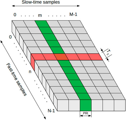
As shown in Figure 2, the samples can be arranged in a 2D matrix. N samples in each column are called fast-time samples, and they correspond to a single transmitted chirp. The samples in rows are called slow-time samples, and they correspond to multiple chirps.
Figures 2, 7 shows that the value of m remains constant in each column, and the value of n remains constant in each row. Therefore, by applying FFT on fast-time samples, the beat frequency can be easily estimated. The term
which makes it easy to estimate the target range using the beat frequency. Finally, to identify the maximum system limit, we use the Rayleigh bandwidth. The Rayleigh bandwidth is 1/T for fast-time samples and 1/MTPRI for slow-time samples; therefore, the range resolution ΔR, the velocity resolution Δv, the maximum unambiguous range Rmax, and the maximum velocity vmax can be easily calculated as follows:
In the following section, the above mentioned derivations will be used to collect samples for extracting the features and estimating ranges and velocities corresponding to different targets.
3 Data Collection and Feature Extraction
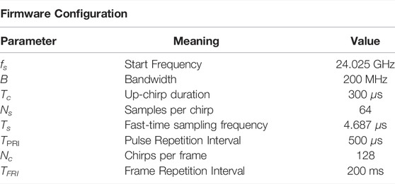
To collect samples for the classifier, we used a commercially available radar module produced by Infineon, called Position2Go (Infineon, 2021). This module is equipped with a 24 GHz transceiver chip (BGT24MTR12) and a 32-bit microcontroller (XMC4700) for signal processing. Three micro-strip series patch antennas (one for transmission and two for reception) are printed on the board. The field-of-view of each antenna is 19, ×, 76°. The basic architecture of the module is similar to the one shown in Figure 1, the only difference is that Position2Go has one transmit and two receive channels. The module is described in detail in (Will et al., 2019). The module’s firmware configuration settings and the specifications for this study are defined in Tables 1, 2.
Figure 3A shows the structure of chirp transmission. Clearly, one frame contains 128 chirps each of duration 300μsec, and chirp repeats itself after pulse-repetition-interval (PRI) of 500μsec. At the receiver end, after the transmission of each chirp, 64 samples were collected. The transmit and receive antennas were not isolated; therefore, the transmit signal was leaked in the receiver that appeared as a low-frequency component in the demodulated signal. This component was independent of the clutter and could be completely removed by storing it in memory and then subtracting it from each column of 2D matrix when the actual experiments were performed. To obtain this signal, it was recommended to point the radar towards an absorbing material or the sky such that only the leakage power signal was received. If the radar was fixed on the ground, it would have been possible to remove the return signal of the background (or clutter). The signals caused by the leakage and background can be removed in a single step by considering a preliminary recording of the scene without the targets

FIGURE 3. Firmware Configuration (A). Hypothetical magnitude of the complex samples in the matrix F along each column, in the case of two scatterers (B).
Subtracting this signal from the received signal in the presence of actual targets in the scene can in fact significantly improve the detection performance
The above mentioned equations are approximately valid when the background return is essentially unaffected by the presence of the targets, and the sensor is fixed on the ground.
Therefore, as shown in Figure 2, the collected 64 complex samples of raw data corresponding to each of 128 chirps can be used to form a 64 × 128 measurement matrix M. After leakage and background removal, a Hamming window is applied to each column for range side-lobe reduction. To limit the straddle loss, each column of the 2D data matrix is zero-padded to
where
To differentiate the moving targets from stationary targets, a technique known as moving target indication (MTI) filtering is used (see (Mark and Richards, 2015)). MTI involves high-pass filtering and can be implemented using the algorithm given in Supplementary Appendix 0.1. Stationary targets do not move from one chirp to another, and they show zero Doppler effects; they cannot be completely removed using MTI filtering alone. Therefore, to remove these targets, before MTI filtering, the mean of each row of F is computed and subtracted from the respective row. We indicate with X the
where
The dimension of vector p simply corresponds to the maximum number of targets that someone is interested in tracking on the same scene.
Each peak index shows the position of a moving target. The phase history Φ of each target is extracted from the corresponding row of the matrix F as follows:
Each Φi is multiplied by a Hamming window, wH, to reduce the side-lobes and is zero-padded to
where
Remark 2: This approach does not require the computation of the complete 2D FFT. Let us assume (N)FFT denotes the total number of operations required to compute the FFT of N elements sequence. We denote by Nc,
In the following section, scattering model of human and cyclist will be discussed and samples in dis will be used to extract features.
4 Scattering Model Based Feature Extraction
The Boulic-Thalmann is one of the example of human scattering model, which is based on bio-mechanical experimental data (Boulic et al., 1990; Melvin and Scheer, 2013). As per this model, the human echo can be approximated by the superposition of N distinct point-scatterers, each with its own dynamics.
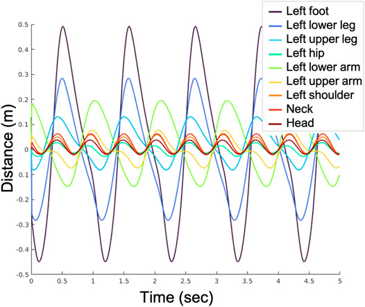
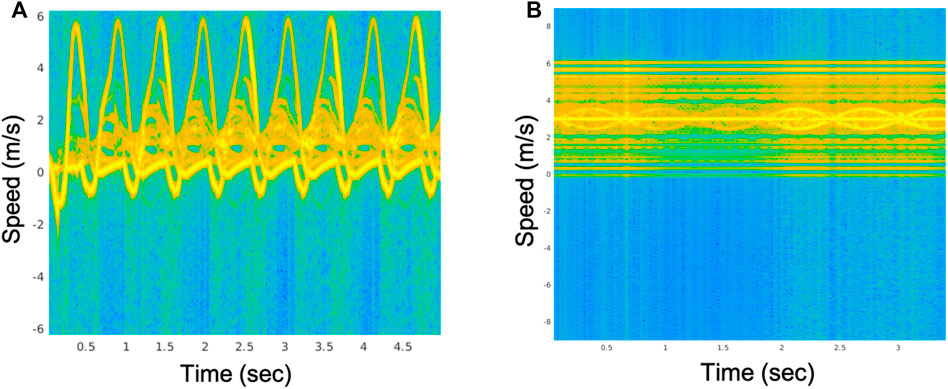
In (Tahmoush et al., 2010), a 16 points scattering model of a 1.8-m tall person walking at 1.5 m/s, as shown in Figure 4, is discussed. Figure 5 and Figure 6A show the movement of the corresponding simulated limbs and time-frequency spectrum, respectively. Similarly, a kinematic model of a cyclists has been developed in (Stolz et al., 2017). Figure 6B shows the simulated time-frequency spectrum of a cyclist traveling at 3 m/s. Here, we can see that multiple frequencies are present, in addition to the time-evolving frequencies that can be attributed to the motion of the legs and pedals. These frequencies spread from 0 m/s to twice the cyclist’s speed and are attributed to the signals returning from the wheels. The torsos and heads of the cyclists and pedestrians are responsible for the dominant return. Because of the relative motion of the various body parts with respect to the torso, multiple Doppler frequencies appear in the spectrum; this effect is known as the micro-Doppler effect (see (Chen et al., 2003)).

FIGURE 4. Sixteen point-scatterers body approximation model. Subfigures (A–C) shows how scatterers change locations with respect to person’s movement.
The spectrum of the signal’s return reveals the periodicity T of limbs’ kinematics, which is usually in the order of seconds. Unmodulated CW radars are best suited for time-frequency analysis; however, they require long windows to capture low frequencies. Nevertheless, FMCW radars typically transmit multiple short waveforms in a frame over a long duration. Because of the short time window, the Doppler frequencies captured during the transmission of one frame are almost constant. With sufficient velocity resolution, sufficient Doppler information could be captured for the classification.
Considering these factors, we designed two subsets with low-complexity features. The first subset captures the number, strength, and distribution of peaks in the current Doppler spectrum. The second subset captures feature variations in the current and previous Doppler spectrums. None of the features are based on the ego speed of the target, i.e., the target’s actual speed. To extract the features, we first determine the 512-point FFT of the corresponding row for each selected index pi of the matrix F, i = 1, 2, …, 5. This spectrum specifies the Doppler frequencies associated with the target present in the pi index location, and it is denoted by D. compactness,
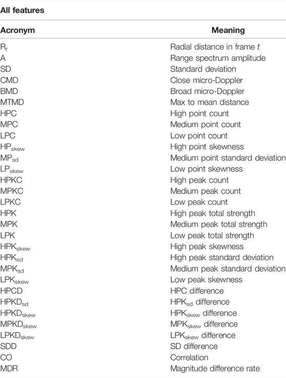
The first subset includes also the following simple threshold-based features HPC, MPC, LPC, HPskew, MPsd, and LPskew. The pseudo-code to identify these features is then described in Supplementary Appendix 0.3, where an approach similar to the one in (Hyun and Jin, 2020) is used. Finally, the first subset contains the following “twin” advanced threshold-based features HPKC, MPKC, LPKC, HPKskew, HPKsd, MPKsd, LPKskew, HPK, MPK, and LPK. These features consider the number of peaks contained in the intervals defined by the thresholds, rather than merely considering the number of spectrum points. The pseudo-code used to identify these features is described in Supplementary Appendix 0.4. The features determined so far are based only on a single frame. To improve the prediction accuracy, the second subset of features measures the numerical variations of certain features over two subsequent frames. For the differential features defined as HPCD, HPKDsd, HPKDskew, MPKDskew, LPKDskew, SDD, CO, and MDR, the pseudo-code is described in Supplementary Appendix 0.5. The reason to select these features can be understood by looking at Figure 6. We observe that, at any instant, there are numerous strong peaks in the pedestrian’s Doppler spectrum; this is captured by features like HPC, HPKC, and HPK. We can also observe that the distribution of the peaks around the pedestrian’s body speed tends to be very skewed in one direction, unlike what we can observe in the cyclist’s Doppler spectrum: this is captured by features like HPskew and HPKskew. Moreover, this skewness varies a lot from one frame to the next one: this is captured by features like HPKDskew. The distribution and deviation of the peaks from the strongest frequency present in the Doppler spectrum are also captured by features like SD, CMD, BMD, and MTMD. The contribution of the wheel’s motion is much lower in amplitude than the contributions of the bike’s frame and cyclist’s body; obviously, this characteristic can’t be observed in the Doppler spectrum of a pedestrian: this is captured by features like LPC, LPKC, and LPK.
To select these features, let us assume that a set of No labeled observations each of feature length l are available for a classification problem. We denote this set by X. Feature selection is a procedure that identifies a column subset with cardinality g < l. Mathematically, if
Feature selection is useful to reduce the dimension of the data set; however, most importantly, it helps identify the relevant features. Viable feature selection algorithms depend on the model selected for the classification. We used sequential feature selection for Ridge Classification and KNNs having the radial basis function. Similarly, for classification and regression tree (CART) ensemble trees, model-based feature selection is used. Sequential-feature-selection (SFS) is a suboptimal recursive method to sequentially add (or subtract) relevant (or irrelevant) features (see (Ferri et al., 1994)). Forward SFS is a greedy method that maximizes a criterion function by recursively adding locally optimal features. However, MBFS is usually faster when it is possible to directly measure the importance of a feature from the model as per a given criterion.
5 Experimental Results
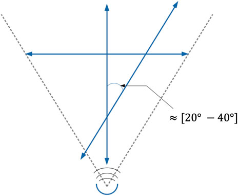
Data were gathered in an area where there was ample space such that the clutter effect was minimized. The sensor was positioned on a tripod at the height of 1.3 m. We considered two pedestrians, two cyclists, and two car models. Each target was recorded while moving in three directions: radial, diagonal, and perpendicular (or azimuthal) as shown in Figure 7.
Data were collected during the day and at night. As shown in Table 4, we recorded 5,123 frames; moreover, the detection was limited between 5 and 25 m.

TABLE 4. Number of frames captured for machine learning algorithms when different targets move in radial, diagonal, and perpendicular directions.
5.1 Radial Data
First, we provide a general overview of radar data before and after processing. Figure 8A shows the unfiltered range profile for a pedestrian walking in the radial direction with respect to the radar. The Fourier transform spectrum of fast-time samples for the first chirp from each frame are aligned and distributed as per the corresponding instant of transmission. From Figure 8A, when the pedestrian is clearly close to the radar at the time zero, the amplitude of the reflected signal is high; with the passage of time, the amplitude of the return decreases because of the pedestrian’s motion away from the radar. When the pedestrian covers a distance of 40 m, the reflected signal from the pedestrian becomes negligible. After 25 s, the pedestrian takes a “U″ turn and returns in the direction of the radar; therefore, the reflected signal from the pedestrian starts to increase. After 52 s, the pedestrian returns to the radar with the maximum reflected signal. Figures 8A–C show that at high ranges, the target peak is obscured in the nearby slowly-moving and static targets. To reduce the contribution of static and slowly moving targets, we use MTI and DC filtering; the output is then shown in Figures 8D–F. We see how the strength of the moving target increased compared to the static background. The gain is particularly visible for large distances. Figures 8A,D show the similar plots for pedestrians moving in the radial direction. Figures 8B,E show similar plots for cyclists moving in the radial direction, and Figures 8C,F show similar plots for the car moving in the radial direction.
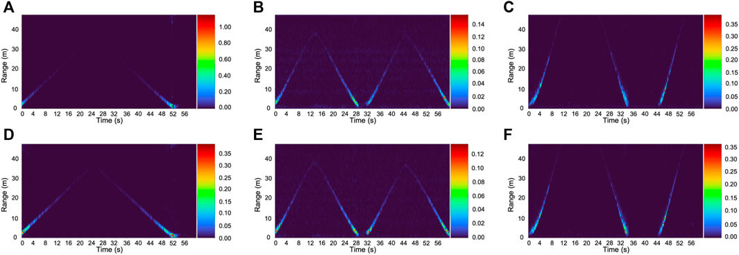
FIGURE 8. Range spectra before (first row) and after (second row) filtering of a pedestrian (A,D), a cyclist (B,E), a car (C,F).
After detecting the target, the Doppler spectrum is computed as previously described. To obtain a more infor¬ mative plot, distance attenuation is compensated for by multiplying the Doppler spectrum with the square of the distance of the target. Figures 9A–C, show a plot of the Doppler spectrum versus the transmission time.
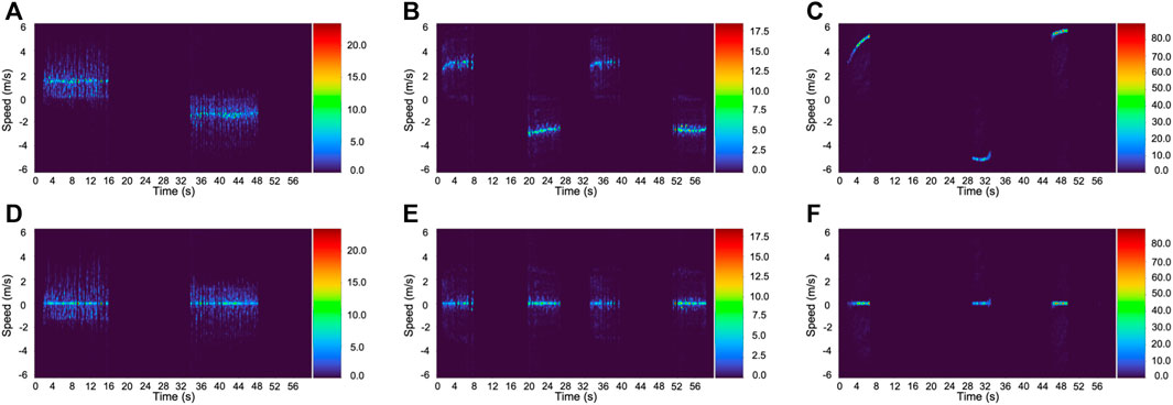
FIGURE 9. Original Doppler spectrum (first row) and after centering the Doppler spectrum to zero (second row) of a pedestrian (A,D), a cyclist (B,E), a car (C,F).
In Figures 9D–F, the Doppler spectrum’s strongest component associated with the pedestrian’s torso, the cyclist’s torso, and the car frame was centered at 0 m/s. Despite the short frame duration supported by our sensor, the most important trait of spectrograms shown in Figures 6A,B were captured. The Doppler spectrum of a pedestrian typically contains multiple relevant frequencies because limbs are in motion while walking. Furthermore, the asymmetry (or skewness) in the distribution of these frequencies around the torso was captured. For a cyclist, the strongest Doppler components are located extremely close to the torso’s Doppler. Moreover, the weak frequencies are extensively distributed because of the wheel’s return. Finally, the Doppler spectrum of a car shows the return of the car’s frame. Moreover, extremely weak Doppler components can be observed because of wheels. Unlike the case for a bicycle, a portion of a car’s wheels is typically obscured by the bumper. Consequently, only the lowest part of the wheel is exposed, and the corresponding Doppler frequencies are asymmetrically distributed around the Doppler of the car’s frame.
5.2 Radial Models
For Ridge Classification and KNNs, we depended on the Scikit-learn implementations (Pedregosa et al., 2015), whereas for the CART Tree Ensembles, XGBoost (Chen and Guestrin, 2016) was used. The selected features are extracted from the targets arranged in the data matrix

FIGURE 10. Feature number versus accuracy for Ridge (A), KNN (B), and XGBoost (C), using radial data only.
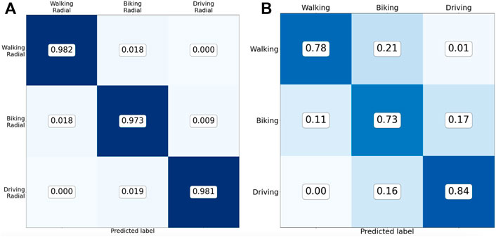
FIGURE 11. Confusion matrix on the test data set using the best sixteen of our proposed features (A), confusion matrix using the features proposed in (Hyun and Jin, 2020) (B). For both cases we used an XGBoost model.
The results of our proposed approach are compared with the three feature approach proposed in (Hyun and Jin, 2020) for the human and vehicle classification. In this approach, the first feature x1 maintains the number of Doppler spectrum points above a certain threshold. The second feature x2 maintains the variation in x1 from frame to frame, and the last feature x3 keeps the echo’s power fluctuation from frame to frame. Typically, the pedestrian’s Doppler spectrum contains many Doppler frequencies because of the multiple body points in motion, whereas the car’s Doppler spectrum typically contains a single dominant frequency. Therefore threshold-based features confirm to be extremely effective to distinguish these targets. The introduction of cyclists helped modify and expand this approach. The Doppler spectra of cyclists and pedestrians demonstrate multiple common traits. The application of features proposed in (Hyun and Jin, 2020) afforded us the scores shown in Figure 11B.
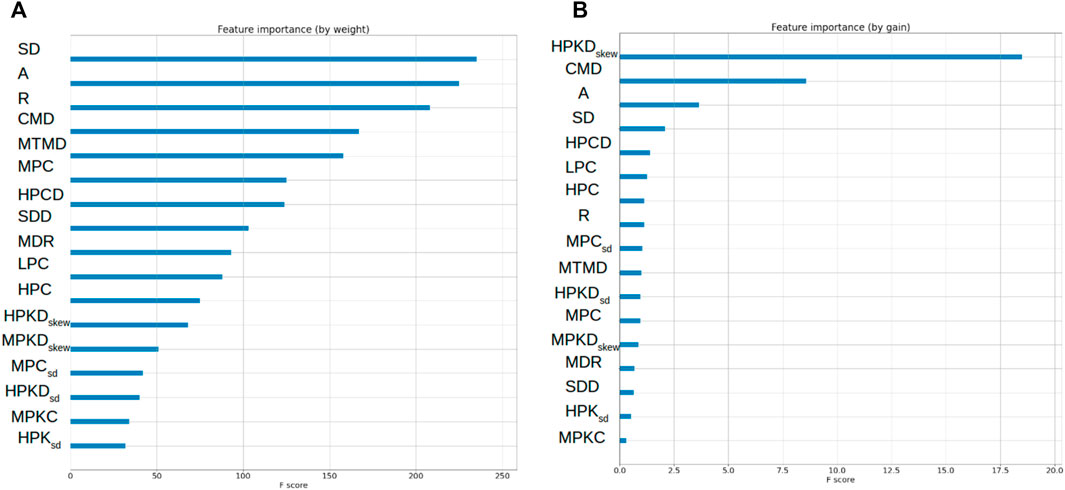
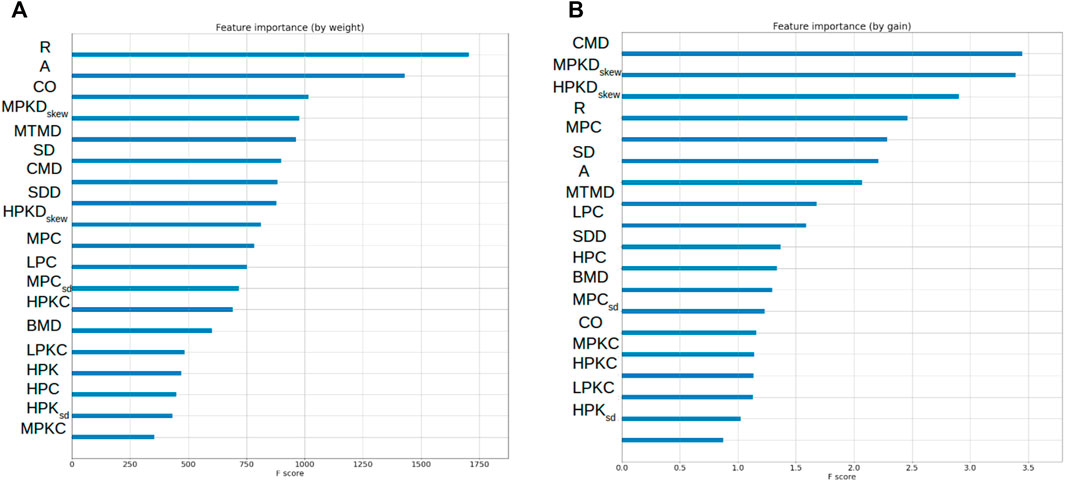
Algorithm 1. SFS model training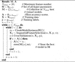 Comparing the confusion matrices of both approaches, we can clearly see that the results obtained by our approach offers higher accuracy than other approaches. Furthermore, graphs in Figures 12A,B, show ranking by importance for each feature.
Algorithm 2. MBFS model training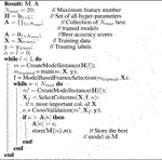
5.3 Multi-Directional Data
We extended our model to consider all three directions, as shown in Figure 7. Figure 13 shows the Doppler spectra. For the diagonal motion, the primary characteristics of the pedestrian and cyclist are preserved; however, the exposure of the car’s wheels to the field of view of the radar makes the spread of weak frequencies more prominent and reduces the asymmetry, as shown in Figure 9C. For perpendicular motion, the Doppler information is minimal. There is a clear similarity between the frequency distributions around the dominant Doppler for the cyclist and car; in fact, we will show subsequently that these two targets can be easily confused by classifiers.
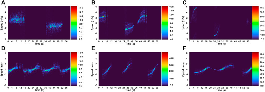
FIGURE 13. Doppler spectra for diagonal motion of a pedestrian (A), a cyclist (B), a car (C) and for perpendicular motion of a pedestrian (D), a cyclist (E), a car (F).
5.4 Multi-Directional Models
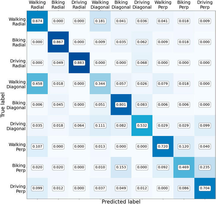
We followed the steps described in Algorithm 1 and Algorithm 2. In addition to target classification, we trained classifiers to predict the direction of motion; consequently, we obtain nine classes. Figures 14A–C shows the corresponding results of each model; these figures show that the average performance was considerably low this time. The highest accuracy on training and testing was achieved by XGBoost. Using 19 features, the classifier scored 63.0% on the test set and 72.6% (the highest) on the train set with the five-fold CV. The confusion matrix in Figure 15 shows that the selected features yield promising results but they are insufficient to reliably predict the target and the direction of motion. However, let’s examine the performance based on target type (pedestrian, cyclist, or car) classification without predicting the direction of motion. Here, very good results can be observed in the confusion matrices shown in Figure 16.
If the target is moving in the radial direction, then an average of 90% cases are correctly classified. The most challenging scenario occurs when the target moves perpendicular to the radar. From Figure 16C, we see that it is difficult to distinguish between the cyclist and car. However, the pedestrian was correctly classified in 84% of cases. In Figure 17, we show the importance of each feature as per the gain and weight.
6 Conclusion
This study explores the role of the commercial radar sensors for classification tasks. We demonstrated that radar technology can offer high accuracy for classifying road users using simple methods that are compatible with low-power applications. In addition to our model, the device can be directly implemented as a surveillance system or can be mounted on a vehicle while the performance levels are preserved. Our proposed algorithm has a few limitations, e.g., if the Doppler information is limited, as for targets moving along the azimuth direction, it will be necessary to consider additional complex features that might be difficult to design and interpret. In our scenarios, all targets moved; this was a necessary condition to exploit the Doppler effect. In future, the robustness of radar-based classification models to static targets can be increased if multiple transmitters and receivers are made available. In such cases, it is important to have access to geometrical information. A demonstration video of the work can be seen at https://www.youtube.com/watch?v=AWY2Fhk7i74.
Data Availability Statement
The original contributions presented in the study are included in the article/Supplementary Material, further inquiries can be directed to the corresponding author.
Author Contributions
SA and RC formulated the problem, while M-SA varified it. Most of the experiments are done by RC, SA was also participating in a few experiments. The initial draft of the paper is written by RC, while SA and M-SA finalized it.
Funding
The KAUST will pay the open access publication fees. The funds are coming from the KAUST Impact grant.
Conflict of Interest
The authors declare that the research was conducted in the absence of any commercial or financial relationships that could be construed as a potential conflict of interest.
Publisher’s Note
All claims expressed in this article are solely those of the authors and do not necessarily represent those of their affiliated organizations, or those of the publisher, the editors and the reviewers. Any product that may be evaluated in this article, or claim that may be made by its manufacturer, is not guaranteed or endorsed by the publisher.
Supplementary Material
The Supplementary Material for this article can be found online at: https://www.frontiersin.org/articles/10.3389/frsip.2022.864538/full#supplementary-material
References
Boulic, R., Thalmann, N. M., and Thalmann, D. (1990). A Global Human Walking Model with Real-Time Kinematic Personification. Vis. Comput. 6, 344–358. doi:10.1007/BF01901021
Chen, T., and Guestrin, C. (2016). “XGBoost: A Scalable Tree Boosting System,” in Proceedings of the 22nd ACM SIGKDD International Conference on Knowledge Discovery and Data Mining, 785–794. doi:10.1145/2939672.2939785
Chen, V. C., Li, F., Ho, S.-S., and Wechsler, H. (2003). Analysis of Micro-doppler Signatures. IEE Proc. Radar Sonar Navig. 150, 271–276. doi:10.1049/ip-rsn:20030743
Cooper, J. (1980). Scattering of Electromagnetic Fields by a Moving Boundary: The One-Dimensional Case. IEEE Trans. Antennas Propagat. 28, 791–795. doi:10.1109/TAP.1980.1142445
Ferri, F. J., Pudil, P., Hatef, M., and Kittler, J. (1994). Comparative Study of Techniques for Large-Scale Feature Selection* *This Work Was Suported by a SERC grant GR/E 97549. The First Author Was Also Supported by a FPI grant from the Spanish MEC, PF92 73546684. Machine Intelligence and Pattern Recognition 16, 403–413. doi:10.1016/B978-0-444-81892-8.50040-7
Hyun, E., and Jin, Y. (2020). Doppler-Spectrum Feature-Based Human-Vehicle Classification Scheme Using Machine Learning for an FMCW Radar Sensor. Sensors 20, 2001. doi:10.3390/s20072001
[Dataset] Infineon (2021). Demo Position2go. Neubiberg, Germany: Infineon. Available at: https://www.infineon.com/cms/en/product/evaluation-boards/demo-position2go/.
Mark, A., and Richards, P. (2015). Fundamentals of Radar Signal Processing, Second Edition, Vol. 53.
Melvin, W. L., and Scheer, J. A. (2012). Principles of Modern Radar: Advanced Techniques. Adv. Tech.. doi:10.1049/SBRA020E
Melvin, W. L., and Scheer, J. A. (2013). Principles of Modern Radar: Volume 3: Radar Applications. Radar Appl. 3. doi:10.1049/SBRA503E
Patel, K., Rambach, K., Visentin, T., Rusev, D., Pfeiffer, M., and Yang, B. (2019). “Deep Learning-Based Object Classification on Automotive Radar Spectra,” in 2019 IEEE Radar Conference, RadarConf (Boston, MA, USA: IEEE), 1–6. doi:10.1109/RADAR.2019.8835775
Pedregosa, F., Varoquaux, G., Buitinck, L., Louppe, G., Grisel, O., and Mueller, A. (2015). Scikit-learn: Machine Learning in Python. J. Machine Learn. Res. 19, 29–33.
Perez, R., Schubert, F., Rasshofer, R., and Biebl, E. (2018). “Single-Frame Vulnerable Road Users Classification with a 77 GHz FMCW Radar Sensor and a Convolutional Neural Network,” in 2018 19th International Radar Symposium (IRS) (Bonn, Germany: IEEE), 1–10. doi:10.23919/IRS.2018.8448126
Richards, M. A., Scheer, J. A., and Holm, W. A. (2010). Principles of Modern Radar. Basic Principles. doi:10.1049/sbra021e
Stolz, M., Schubert, E., Meinl, F., Kunert, M., and Menzel, W. (2017). “Multi-target Reflection point Model of Cyclists for Automotive Radar,” in 2017 European Radar Conference (EURAD) (Nuremberg, Germany: IEEE), 94–97. doi:10.23919/EURAD.2017.8249155
Tahmoush, D., Silvious, J., and Clark, J. (2010). An UGS Radar with Micro-doppler Capabilities for Wide Area Persistent Surveillance. Radar Sensor Technol. 7669, 766904. doi:10.1117/12.848233
Trevor, H., Robert, T., and Jerome, F. (2009). The Elements of Statistical Learning, Vol. 27. Berlin, Germany: Springer.
Will, C., Vaishnav, P., Chakraborty, A., and Santra, A. (2019). Human Target Detection, Tracking, and Classification Using 24-GHz FMCW Radar. IEEE Sensors J. 19, 7283–7299. doi:10.1109/JSEN.2019.2914365
Youngwook Kim, Y., and Hao Ling, H. (2009). Human Activity Classification Based on Micro-doppler Signatures Using a Support Vector Machine. IEEE Trans. Geosci. Remote Sensing 47, 1328–1337. doi:10.1109/TGRS.2009.2012849
Keywords: FMCW, radar, micro-Doppler, machine learning, classification
Citation: Coppola R, Ahmed S and Alouini M-S (2022) Road Users Classification Based on Bi-Frame Micro-Doppler With 24-GHz FMCW Radar. Front. Sig. Proc. 2:864538. doi: 10.3389/frsip.2022.864538
Received: 28 January 2022; Accepted: 29 March 2022;
Published: 20 May 2022.
Edited by:
Danilo Orlando, University Niccolò Cusano, ItalyReviewed by:
Chengpeng Hao, Institute of Acoustics (CAS), ChinaMohammed Jahangir, University of Birmingham, United Kingdom
Copyright © 2022 Coppola, Ahmed and Alouini. This is an open-access article distributed under the terms of the Creative Commons Attribution License (CC BY). The use, distribution or reproduction in other forums is permitted, provided the original author(s) and the copyright owner(s) are credited and that the original publication in this journal is cited, in accordance with accepted academic practice. No use, distribution or reproduction is permitted which does not comply with these terms.
*Correspondence: Sajid Ahmed, c2FqaWQuYWhtZWRAa2F1c3QuZWR1LnNh
 Rudi Coppola
 Sajid Ahmed
 Mohamed-Slim Alouini
