Multi-environment trials data analysis: linear mixed model-based approaches using spatial and factor analytic models

The analysis of multi-environment trials (MET) data in plant breeding and agricultural research is inherently challenging, with conventional ANOVA-based methods exhibiting limitations as the complexity of MET experiments grows. This study presents linear mixed model-based approaches for MET data analysis. Ten MET grain yield datasets from national variety trials in Ethiopia were used. Randomized complete block (RCB) design analysis, spatial analysis, and spatial+genotype-by-environment (G × E) analysis were compared under linear mixed model framework. Spatial analysis detected significant local, global, and extraneous spatial variations, with positive spatial correlations. For the spatial + G × E analysis, increasing the order of the factor analytic (FA) models improved the explanation of G × E variance, though the optimal FA model order was dataset-dependent. Integrating spatial variability through the spatial + G × E modeling approach substantially improved genetic parameter estimates and minimized residual variability. This improvement was particularly notable in larger datasets, where the number of trials and the size of each trial played a crucial role for presence of spatial variability and strong GxE effects. Additionally, the genetic correlation heat maps and dendrograms provided intuitive insights into trial relationships, revealing patterns of strong positive, negative, and weak correlations, as well as distinct trial clusters. The results clearly demonstrate that linear mixed model-based approaches, especially the spatial + G × E analysis excel in capturing complex spatial plot variation and G × E effects in MET data by effectively integrating spatial and FA models. These insights have important implications for improving the efficiency and accuracy of MET data analysis, which is crucial for improving genetic gain estimation in plant breeding and agricultural research, ultimately accelerating the delivery of high-performing crop varieties to farmers and consumers.

1 Introduction

Crop variety development is a fundamental pillar of modern agriculture, with advancements over the past century playing a vital role in enhancing global food security, improving farmer livelihoods, and promoting sustainable farming practices (Qaim, 2020; Begna and Begna, 2021). By creating high-performing, adaptable cultivars that are resilient to biotic and abiotic stresses, researchers have enabled stable and abundant crop yields, bolstered food supplies, and supported the economic wellbeing of farming communities, while also facilitating the adoption of other sustainable agricultural innovations (Zsögön et al., 2022; Swarup et al., 2021). Continued investment and innovation in this field will be crucial as the world navigates the complex challenges of ensuring long-term food security and environmental sustainability (Blakeney, 2022).

Multi-environment trials (METs) are a crucial element of the crop variety development pipeline. In this process, newly bred crop genotypes are evaluated across a range of agro-ecological environments (Smith et al., 2001b, 2021; Brown et al., 2020). The primary purpose of METs is to capture the influence of diverse environmental factors on the expression of genotypic performance. This allows for the assessment of G × E effects- a critical consideration in identifying high-performing and stable crop varieties that can perform well under a range of conditions (Verbyla, 2023; Lee et al., 2023; Lisle et al., 2021).

Understanding G × E is a fundamental aspect of plant breeding, as it provides insights into how different genotypes respond to diverse environmental conditions. This interaction is critical because it directly affects important agronomic outcomes, such as yield and the ability of plants to adapt to varying climates and soil types (Van Eeuwijk et al., 2016; Malosetti et al., 2013, 2016; Bustos-Korts et al., 2009). This is also demonstrated in studies by Cooper et al. (2020); Mark et al. (2021) and Cooper et al. (2022) that focus on implementing management strategies to maximize crop productivity through combinations of Genotype–Management (G–M) technologies.

By testing new genotypes across multiple environments, breeders can gain valuable insights into how a variety's traits manifest and interact with the local environmental context. This information is essential for selecting cultivars that exhibit both high productivity and reliability, making them suitable for deployment across a wide geographical area (Smith et al., 2001b, 2019, 2021).

The conventional approach for analyzing MET data has relied on ANOVA-based methods, such as AMMI (additive main effects and multiplicative interaction) and GGE (genotype and genotype-by-environment interaction) analysis (Beeck et al., 2010; Zhang et al., 2020). These techniques have enabled researchers to obtain ANOVA results and gain insights into interactions. Additionally, they have facilitated data visualization through the use of biplot techniques.

However, these methods exhibit several inherent limitations that have become increasingly apparent as the complexity of MET experiments has grown. One key issue is that ANOVA-based methods may struggle to handle unbalanced and incomplete data structures, where some observations are missing or not all genotypes are present in each environment (Piepho, 1997; Smith et al., 2001a; Kelly et al., 2007). This is a common challenge in MET studies. Additionally, these methods may fail to adequately account for non-genetic sources of variance associated withenvironmental factors or experimental design effects, which can significantly influence the observed phenotypic performance (Smith et al., 2005). Furthermore, the ANOVA-based analysis commonly follows a two-stage modeling approach. This involves first analyzing the data within each environment, followed by a second stage of combining the results across environments for the G × E interaction analysis (Piepho et al., 2012; Smith et al., 2005). This approach can lead to a loss of information and less effective extraction of insights from the complex MET datasets.

Linear mixed model-based approaches have emerged as a more efficient methodology for the analysis of MET data. Recently, these mixed model approaches have become predominant, as they provide a flexible framework that can easily handle incomplete data and appropriately model the non-genetic variances between and within environments. This includes accounting for spatial variation within environments and error variance heterogeneity across environments (Smith et al., 2001a). The error variation within environments can be modeled using the approach of Gilmour et al. (1997), which appropriately models the three patterns of spatial trends associated with the field of trials: local, extraneous, and global trends.

Smith et al. (2001a, 2005) extended the G × E analysis by employing Factor Analytic Multiplicative Mixed (FAMM) models. These models assume random genotype effects and fixed environment effects, and use a one-stage analysis approach, where the models for residual effects are estimated simultaneously with the models for G × E effects. A key feature of the Factor Analytic (FA) model for MET data is its importance for the estimation of the associated variance structure for G × E effects. The FA model provides a good and parsimonious approximation to the unstructured form, and is generally more computationally robust (Kelly et al., 2007). Additionally, the best linear unbiased predictions (BLUPs) of the G × E effects and estimations of loadings and scores can be obtained, enabling bi-plot analysis to better understand the G × E interaction patterns.

The objective of this research is to explore the potential of linear mixed model-based approaches, particularly FAMM models, as a high-performing alternative to the traditional randomized complete block (RCB) designs analysis for effectively analyzing MET data and extracting meaningful insights from the complex G × E interactions. By leveraging linear mixed model-based methodology, this research aims to demonstrate how the non-genetic variances within and between environments can be appropriately modeled, including the use of the Gilmour et al. (1997) approach for capturing spatial trends and error variation. Furthermore, the application of FAMM models is explored, as these approaches provide advantages in estimating the variance structure of G × E effects and enabling more informative visualizations. The ultimate goal is to provide researchers and breeders with a robust and efficient analytical tool for extracting meaningful insights from MET data, ultimately supporting the development of high-performingand adaptable crop varieties.

2 Data and methods

2.1 Motivating data

The study utilized 10 MET datasets from the national variety trial (NVT) series conducted by the Ethiopian Institute of Agricultural Research (EIAR). All trials were laid out in RCB design with a rectangular array of plots, and were carried out across various locations in Ethiopia between 2014 and 2020. The trials were conducted by the research programs for common bean, chickpea, wheat, and maize. Each trial had a minimum of two replicates per entry. The terms “trial” and “environment” are used interchangeably, referring to a unique year-location combination. The trait analyzed in this study was harvested grain yield, measured in tons per hectare. There was a high degree of concurrence, or overlap, between entries both within and across years. The name of each dataset was designated using the first letter of the trial series name, two letters for the crop name, and the last two digits of years for the duration of the trial series (Table 1). Both complete datasets, where all entries were grown in all trials, and incomplete datasets were considered in the analysis. The complete datasets included LCB14-16, ACB14-16, SCB14-16, and BWT19-20. The total number of environments (year-location combinations) ranged from 8 to 16 across the different datasets.

Table 1

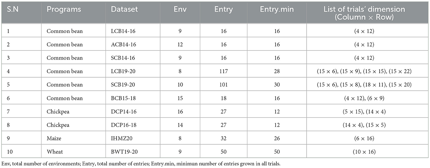
Table 1. Summary of ten MET datasets.

2.2 Statistical models

ANOVA-based models have long been used for the analysis of MET data, providing a foundational approach to understanding genotype performance across different environments. The general statistical models for these techniques allow for the estimation of mean effects, genotype interactions, and random error components. Recently, linear mixed model-based approaches have become increasingly useful for analyzing complex MET data sets, as they can incorporate both fixed and random effects, accommodating variability in the data. In this section, we first present the general statistical model for ANOVA-based methods, followed by the statistical models for linear mixed model-based approaches, emphasizing their statistical applications in MET data analysis.

2.2.1 ANOVA based models

The base-line statistical model for MET data analysis can be written as

$\begin{array}{ll}\begin{array}{c}{y}_{ikj}={\eta }_{ij}+{\beta }_{kj}+{\epsilon }_{ikj}\\ {\eta }_{ij}=\mu +{\alpha }_i+{\delta }_j+{\gamma }_{ij}\end{array}& (1)\end{array}$

where y_ijk is yield of the i^th entry of replicate block k in environment j (i=1, 2…m, j=1,2…t, k=1,2…r), η_ij is the empirical/least-square mean effect of entry i in environment j, μ is an overall mean effect, α_i is the main effect for genotype i, β_kj is the block effect at trial j, γ_ij is the interaction effect for genotype i in trial j, ε_ikj is the random error effect for genotype i in replicate block k of trial j, assumed to be $N(0,\sigma 2)$. The analysis of this model follow the approaches of two stage data analysis, in which the two-way table means η_ij are estimated first from the individual trial's analysis, and then the G × E analysis using GGE or AMMI model. The models for the second stage analysis can be written as

$\begin{array}{ll}{\gamma }_{\text{ij}}=({\eta }_{ij}-(\mu +{\alpha }_i+{\delta }_j))={\displaystyle \sum _{i=1}^c}{\lambda }_l{\tau }_{il}{\theta }_{jl}+{\zeta }_{ij}& (2)\end{array}$

$\begin{array}{ll}({\alpha }_l+{\gamma }_{ij})=({\eta }_{ij}-(\mu +{\delta }_j))={\displaystyle \sum _{i=1}^c}{\lambda }_l{\tau }_{il}{\theta }_{jl}+{\zeta }_{ij}& (3)\end{array}$

where l = 1, 2, . . ., c, λ_l is the singular value of the l^th multiplicative or principal component (PC), with c ≤ min(m−1, t), τ_il is the eigenvector of genotype i for PC l, θ_jl is the eigenvector of environment j for PC l, and ζ_ij is the residual associated with genotype i in environment j, assumed to be NID(0, σ²/r) where r is the number of replications within an environment. The models are subject to the constraints λ1 ≥ λ2, ..., λc ≥ 0 and orthogonally constraints on the τ_il scores, that is $\sum _{i=1}^c{\lambda }_l{\tau }_{il}{\tau }_{i^{\prime }l}$ = 1 if i = i′ and $\sum _{i=1}^c{\lambda }_l{\tau }_{il}{\tau }_{i^{\prime }l}$ = 0 if i ≠ i′ with similar constraints on the θ_jl scores by replacing symbols (i, m, τ ) with (j, s, θ). AMMI analysis may use the model in Equation 2 whereas GGE analysis may use the model in Equation 3.

2.2.2 Linear mixed models

A general form of linear mixed model for the n × 1 vector y of individual plot yields combined across trials can be written as

$\begin{array}{ll}\text{y}=X\tau +Z_g{u}_g+Z_o{u}_o+\epsilon & (4)\end{array}$

where τ is the a × 1 vector of fixed effects, u_g is an mt × 1 vector of random G × E effects with associated design matrix Z_g, u_o is a b x 1 vector of (non-genetic) random effect with corresponding design matrix Z_o, ε is the n × 1 vector of residual error across all trials. Some statistical assumptions are made about the random terms of the general linear mixed models. Thus, we assume that u_g, u_e and ε are mutually independent and have a multivariate normal distribution with zero means vectors and variance matrices var(u_g) = Gg, var(u_e) = Go and var(ε) = R.

The random non-genetic effects u_o can be considered as sub-vectors ${u_{oj}}^{(b_j\times 1)}$ for each trial, where b_j is the number of random terms for trial j. These random terms are based on the terms for the blocking structure (e.g., replicate blocks or rows and columns of the field). In the analysis of MET data, the sub-vectors of u_o are typically assumed to be mutually independent, with variance matrix G_ojfor trial j that has a block diagonal form. Thus, there is a variance matrix$G_o={{\oplus }^t}_j{G}_{oj}$ for the set of none-genetic effects at each trial j.

The variance matrix for resdual effects is assumed to be $R={\otimes }_{j=1}^t{R}_j$ where R_j is the variance matrix for the j^th trial. Individual trial residual effects can be analyzed employing spatial methods of analysis that account for local or plot-to-plot variation. Each R_jin this case will have its own spatial covariance structure (Gilmour et al., 1997). Varietal trials that have row by column arrangement and ordered as rows within columns allow separable spatial models of the form.

$\begin{array}{ll}{R}_j={\sigma }_j^2{\Sigma }_{c_j}({\rho }_{c_j})\otimes {\Sigma }_{r_j}({\rho }_{r_j})& (5)\end{array}$

where and Σ_rj represent spatial correlation structures with parameters in ρ_cj and ρ_rj for the column and row directions, respectively. In both the column and row directions, we typically use an autoregressive spatial structure of order one, with ρ_cj and ρ_rj each containing a single autocorrelation parameter. For spatial auto-correlation in the row direction only, the model simplifies to $R_j={\sigma }_j^2{I}_{n_{cj}}\otimes {\Sigma }_{r_j}({\rho }_{r_j})$ where is the number of columns for trial j. Similarly, $R_j={\sigma }_j^2{\Sigma }_{c_j}({\rho }_{c_j})\otimes I_{n_{rj}}$ would be the reduced form for spatial auto-correlation in the column direction only where n_rj is the number of rows for trial j. We can have also no spatial covariance in either direction. Thus, the model simplified to an IID variance structure of the form.

Smith et al. (2001a, 2005) presented an alternative parsimonious model for u_gusing a factor analysis model to provide a variance structure for the genetic variance matrix. This model can adequately represent the nature of heterogeneous variances and covariances found to occur in most MET data. Thus, the u_g can be modeled with multiplicative terms. That is

$\begin{array}{l}{u}_g=({\lambda }_1\otimes I_m)f_1+...+({\lambda }_d\otimes I_m)f_d+\xi \\ =(\Lambda \otimes I_m)f+\xi & (6)\end{array}$

where λ_h is the t×1 vector of loadings, f_h is the m×1 vector of factor scores (h = 1...d), ξ is the mt×1 vector of residuals, Λ is the t×d matrix of loadings {λ₁ . . . λ_d} and f is the md×1 vector of factor scores ${({f_1}^{\prime }{f_2}^{\prime }...{f_d}^{\prime })}^{\prime }$. The random effects f and ξ are assumed to follow a normal distribution with zero mean vector and variance-covariance matrix.

$\begin{array}{ll}\left[\begin{array}{cc}{G}_f\otimes I_m& 0\\ 0& \text{Ψ}\otimes I_m\end{array}\right]& (7)\end{array}$

where Ψ is a diagonal matrix of specific variances represents the residual variance not explained by the factor model, that is Ψ = diag (Ψ₁ . . . Ψ_t). The factor scores are commonly assumed to be independent and scaled to have unit variance, so that G_f = I_d. The genetic effects u_g can be considered as a two dimensional (genotype by environment) array of random effects, and can be assumed to have a separable variance structure for the (mt × mt ) variance matrix G_g which can be written as

$\begin{array}{ll}{G}_g={\text{G}}_{\text{e}}\otimes G_g& (8)\end{array}$

where G_e is the t×t genetic variance matrix representing the variances at each trial and covariances between trials, and G_g is them×m symmetric positive definite matrix represents variances of environment effects at each genotype and the covariances of environment effects between genotypes. It is typically assumed that the varieties are independent and that G_g = I_m. However, if the pedigree information of the varieties is available, other forms of G_g can be applicable (Smith et al., 2001a; Oakey et al., 2006, 2007). Based on Equation 2 the variance of genetic effects would be

$\begin{array}{l}var(u_g)=(\Lambda {\Lambda }^{\prime }+\text{Ψ})\otimes I_m\\ ={\text{G}}_{\text{e}}\otimes I_m& (9)\end{array}$

Thus, the FA model approach results in the following form for G_e.

$\begin{array}{ll}{G}_e=\Lambda {\Lambda }^{\prime }+\text{Ψ}& (10)\end{array}$

In the model, the variance parametric in these variance matrices are directly estimated using REML estimation method.

2.2.3 Heritability formula

According to the methodology outlined by Cullis et al. (2006), the heritability ($H_j^2$) value for the j^th trial can be calculated from a generalized formula that is employed within the context of linear mixed model analysis. This formula is as follows:

$\begin{array}{ll}{H}_j^2=1-\frac{A_j}{2{{\sigma }_{gj}}^2}& (11)\end{array}$

where A_j is the average pairwise prediction error variance of genetic effects for the j^th environment and ${{\sigma }_{gj}}^2$ is the genetic variance at environment j.

2.3 Statistical inferences, analysis procedures and software

Fitting a linear mixed model involves estimating the values of the fixed effects (τ), a random G × E effects (u_g), the random non-genetic effects (u_o), as well as the variance-covariance parameters in G_g, G_o, and R. This estimation process comprises two interconnected steps. First, the variance parameters of the model are estimated using Residual Maximum Likelihood (REML), an approach introduced by Patterson and Thompson (1971). Second, the fixed and random effects are estimated using distinct techniques—Best Linear Unbiased Estimation (BLUE) is employed for the fixed effects, while Best Linear Unbiased Prediction (BLUP) is used for the random effects.

To assess the statistical significance of the random effects in the linear mixed model, the Residual Maximum Likelihood Ratio Test (REMLRT) can be utilized. However, it is important to note that the REMLRT is only applicable when comparing the fit of two nested models that share the same fixed effects structure. On the other hand, the significance of the fixed effects can be determined using the Wald test. The classic Wald statistic follows an asymptotic chi-squared distribution. Yet, this test has been found to be somewhat anti-conservative in certain scenarios, as reported by Butler et al. (2009). To address this issue, Kenward and Roger (1997) proposed an adjusted Wald statistic and an approximation based on the F-distribution, which have demonstrated improved performance across various settings.

The data analysis process began with the fitting of a randomized complete block (RCB) model. This initial model included random effects for block/replication and variety, and the residual correlation structure was specified as id(Column).id(Row), where 'id' refers to the identity matrix. The next step was to conduct a spatial analysis. First, a spatial model was fitted to the residuals from the RCB model. This spatial model used a separable autoregressive process in the column and row dimensions to account for local variation in the data.

After fitting the spatial model for local variation, a second spatial model was then fitted to capture the extraneous variation along the column and row dimensions. In this model, only the significant terms for local variation were retained. To assess the statistical significance of the fitted spatial models, both for the local and extraneous variation, the Residual Maximum Likelihood Ratio (REMLR) test was employed. Finally, spatial models were fitted to account for the global variation in the data, and the significance of these global spatial models was evaluated using the Wald test.

The other analysis procedure was a spatial + G × E analysis, which was done by incorporating the spatial terms identified in the spatial analysis and modeling the G × E effects using model fitting procedures demonstrated by De Faveri (2013) and Smith et al. (2015). In this analysis, a combined model was first fitted, which is a combined form of individual trial models constructed in the spatial analysis. This combined model forms the basis of a sequence of models to be fitted for the G × E analysis, and it helps to organize the trial-specific models in a combined form and to confirm the presence of genetic variance in each trial. If any trial is found to have no genetic variance, it would be excluded from the multi-environment trial (MET) data analysis.

Factor Analytic (FA) models were then considered, while maintaining the spatial models as specified in the combined model. The adequacy of the FA models of several factors (h) was formally tested, as they are fitted within a mixed model framework. A model with h factors, denoted as FA-h, is nested within a model with h+ 1 factors. The models were compared, such as FA-1 vs. FA-2, FA-2 vs. FA-3, and so on. Both the Residual Maximum Likelihood Ratio Test (REMLRT) and total percentage of the G × E variance (%var) explained by factor components were used to identify the final plausible FA models.

The licensed version of the ASReml-R statistical software package was used to fit all models analyzed in this study (Butler et al., 2009). ASReml-R is a specialized software application designed for fitting linear mixed models, which was well-suited for the data and research questions addressed here.

3 Results

3.1 Spatial analysis

Table 2 presents the results of the Wald test, which was used to assess global spatial variation, as well as the REMLR test, which was employed to detect local and extraneous spatial variation. The analysis revealed several instances of significant spatial variations across the trials. For the trial AN19CBN2, there was notable local spatial variation detected along both the row and column dimensions (p < 0.001). Local spatial variation was also present for the trial 2015CNVT-D-CD, which exhibited significant variation along the column dimension (p = 0.022), as well as for the trial AA20BWNE, which showed local spatial variation along the row dimension (p = 0.001).

Table 2

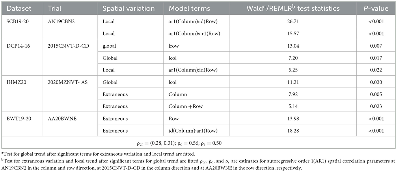
Table 2. Summary of spatial analysis for four trials: spatial variation, fitted model term, Wald and REML test statistic and P-value.

In terms of global linear spatial trends, these were found to be significant along both the row and column dimensions for the trial 2015CNVT-D-CD (p = 0.007 and p = 0.017, respectively) and along solely the row dimension for the environment 2020MZNVT-AS (p = 0.030). Extraneous spatial variation, which cannot be accounted for by linear trends, was detected for the environment 2020MZNVT-AS along both dimensions (p = 0.023) and for the trial AA20BWNE along the row dimension. The estimated AR1 correlations for the significant local spatial terms were all positive (ρ_cr = (0.28, 0.31); ρ_c = 0.56; ρ_r = 0.50).

The heat map visualization of the residual variation for the trial 2020MZNVT-AS, before and after the spatial analysis, is presented in Figure 1. This plot clearly reveals the presence of observable systematic spatial trends within the trial (Figure 1A). The observed spatial trends suggest the presence of extraneous variation that is not adequately accounted for in the initial model. Such systematic spatial patterns are indicative of the need to incorporate random row and column effects, as well as fixed linear global trends, into the linear mixed models (Figure 1B).

Figure 1

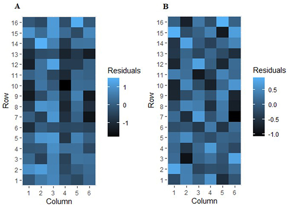
Figure 1. Residual variation heat map before (A) and after (B) spatial analysis for trial 2020MZNVT-AS.

3.2 Spatial + G × E analysis

The results of the factor analytic (FA) model comparisons from the Spatial + G × E analysis for each dataset are presented in Table 3. This includes the residual log-likelihoods (LR), residual maximum likelihood ratio tests (REMLRT), and the total percentage of the G × E variance explained by the FA model (%var).

Table 3

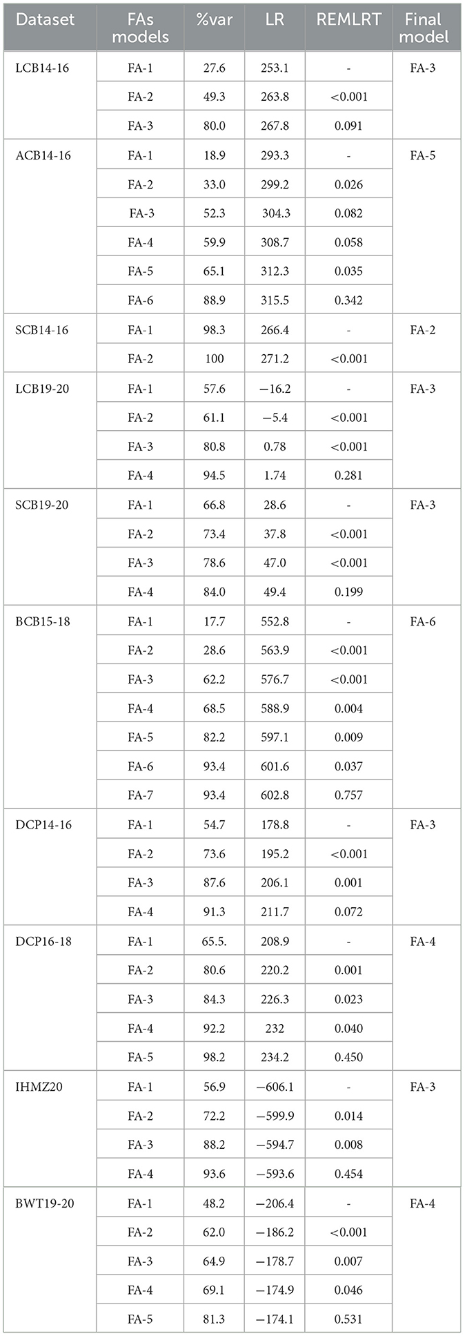
Table 3. FA model comparisons through the total percentage of the G×E variance (%var) explained by the FA components, residual log-likelihoods (LR), and residual maximum likelihood ratio tests (REMLRT).

The analysis revealed that increasing the order of the FA model consistently improved the total percentage of G × E variance explained across all datasets. As the order of the FA model was increased, the significance level of the REMLRT generally decreased across most datasets. However, this pattern did not hold true for the ACB14-16 dataset, where the lower-order FA-2 and higher-order FA-5 models were found to be statistically significant, while the intermediate FA-3 and FA-4 models did not reach significance levels.

Notably, the total percentage of G × E variance explained by the last significant order of the FA model was generally >65% for each dataset, with the exception of LCB14-16. For the LCB14-16 data set, the second-order FA-2 model accounted for 49.3% of the G × E variance, which was still statistically significant. In contrast, the higher-order FA-3 model showed a substantial improvement, explaining 80.0% of the G × E variance, but this was not statistically significant.

In the case of the SCB14-16 data set, the analysis determined that the FA-2 model accounted for a remarkable 100% of the G × E variance, with a highly significant p < 0.001. The third-order FA-3 model was also found to be a plausible model for the G × E analysis in the datasets LCB19-20, SCB19-20, DCP14-16, and IHMZ20, as it explained at least 65% of the G × E variance with p ≤ 0.081. For the DCP16-18 and BWT19-20 data sets, the fourth-order FA-4 model was selected as the final model, accounting for 92.2 and 69.1% of the G × E variance, respectively, with statistically significant p-values. In the case of the ACB14-16 data set, the FA-5 model was chosen as the final model, explaining 65.1% of the G × E variance with a p-value of 0.035. Finally, for the BCB15-18 data set, the higher-order FA-6 model was determined to be the most appropriate, accounting for 93.4% of the G × E variance with a p-value of 0.037.

The average genetic and error variance estimates for each dataset, derived from the RCB, spatial, and spatial + G × E analysis, are presented in Table 4. In the RCB analysis, the average genetic variance estimates ranged from 0.050 to 0.984, and the average error variance estimates ranged from 0.072 to 1.746. The spatial analysis produced average genetic variance estimates ranging from 0.049 to 1.009, and average error variance estimates with a minimum of 0.065 and a maximum of 1.571. From the spatial + G × E analysis, the average genetic variance estimates had a minimum of 0.052 and a maximum of 1.057, while the error variance estimates fell within the range of 0.061 to 1.568. Across all three methods of analysis, the 9IHMZ20 data set exhibited the highest average genetic and error variance, while the 6BCB15-18 data set had the lowest average genetic and error variance.

Table 4

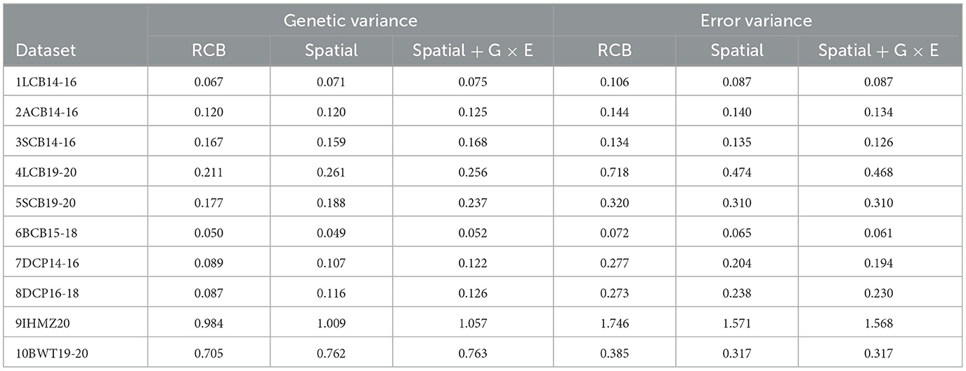
Table 4. A summaries of results from the RCB, Spatial, Spatial + G × E analysis for each MET dataset.

The estimates of genetic variance were observed to improve with the application of spatial analysis, as compared to RCB analysis. More importantly, the spatial + G × E analysis led to substantial improvements in the genetic variance estimates for most of the datasets examined. The spatial analysis provided notably smaller estimates of the error variance compared to the RCB analysis. Interestingly, the spatial + G × E analysis was able to significantly reduce the residual variability, outperforming both the RCB and the spatial methods analysis.

Figure 2 presents the average heritability estimates of yield for each dataset, derived from RCB, Spatial, and Spatial + G × E analysis. The Spatial analysis consistently provided higher heritability estimates compared to the RCB analysis across all the datasets. Furthermore, the spatial + G × E analysis further highly improves the heritability estimates compared to the RCB and Spatial analysis across all the datasets. The extent of improvement from the spatial and spatial + G × E analysis varied among the datasets. Larger improvements were observed for datasets with relatively higher data volumes, such as DCP14-16 (16 trials, 27 entries) and LCB19-20 (8 trials, 117 entries), compared to datasets with lower data volumes, such as LCB14-16 (8 trials, 16 entries) and IHMZ20 (8 trials, 32 entries). While increasing the volume of data generally improves the reliability of statistical estimates and minimizes the risk of misleading conclusions from small sample sizes, it is important to recognize that more data does not inherently ensure that advanced data analysis methods will outperform conventional approaches. The effectiveness of advanced techniques, such as Spatial + G × E analysis, largely depends on the presence of significant factors or sources of variability that need modeling, such as spatial variability or strong G × E interactions.

Figure 2

Figure 2. Average heritability of yield for each dataset using the mixed model analysis: RCB, spatial, and Spatial+G×E analysis.

In our study, we observed that the spatial + G × E method significantly enhanced the analysis, with improvements particularly evident in larger datasets. This finding aligns with the understanding that spatial variability and strong G × E interactions are often more pronounced in larger datasets, a trend frequently observed in Ethiopia's crop MET data, where notable G × E interactions and plot variability are common, as highlighted by Woldemeskel and Fenta (2022) and Taye (2005). Thus, while accumulating more data is beneficial, the true advantage lies in the capacity of advanced methods to capture and model specific sources of variation, especially in larger datasets where these factors become more prominent.

The visualization techniques from the spatial + G × E analysis are presented in Figures 3, 4. Figure 3 displays the heat map representation of the genetic correlation matrix for the dataset SCB19-20 (A), for dataset DCP14-16 (B), for the dataset IHMZ20 (C), and for the dataset BWT19-20 (D). Figure 4 presents the dendrogram representation of the dissimilarity matrix for those same datasets.

Figure 3

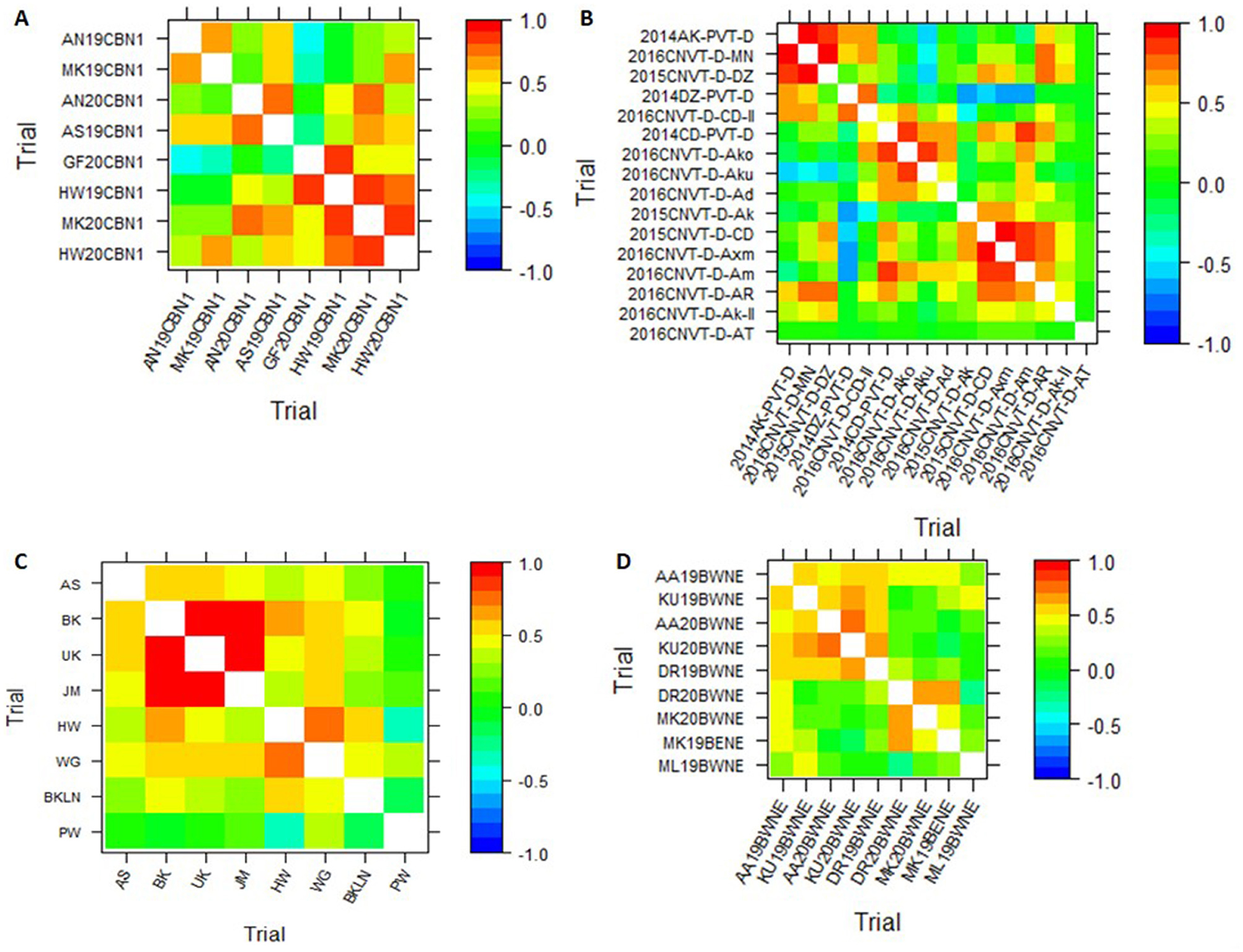
Figure 3. Heat map representation of the genetic correlation matrix from spatial+G×E analysis for the datasets SCB19-20 (A), DCP14-16 (B), IHMZ20 (C), and BWT19-20 (D).

Figure 4

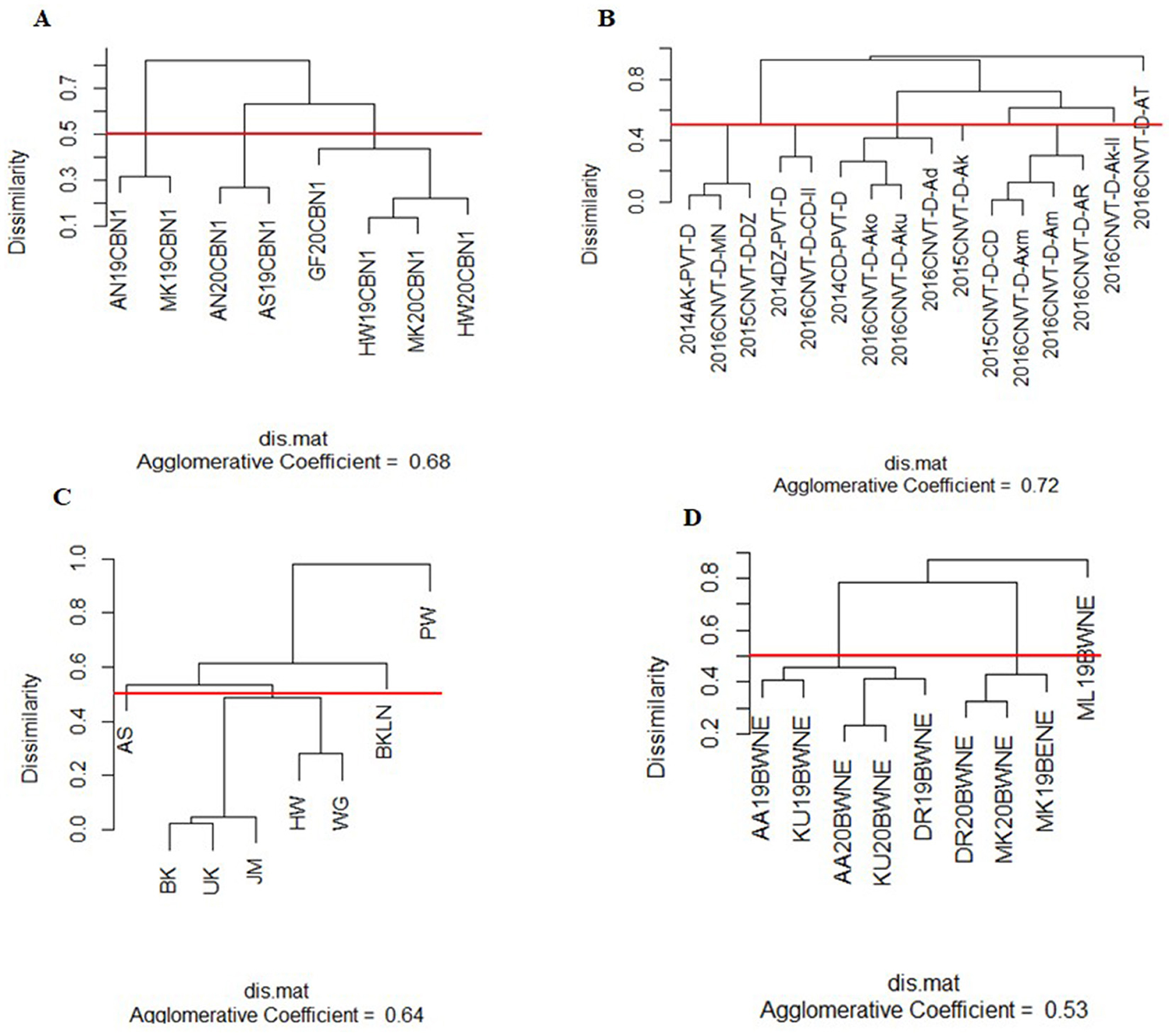
Figure 4. Dendrogram representation of the dissimilarity matrix from spatial+G×E analysis for the datasets SCB19-20 (A), DCP14-16 (B), IHMZ20 (C), and BWT19-20 (D).

The genetic correlation heat map (Figure 3) shows strong positive correlations among some trials within each dataset, denoted by the deep red coloration. Conversely, weak positive and negative correlations are observed for other trial pairings, as indicated by the yellow hues. Additionally, the heat map reveals strong negative correlations between certain trials, represented by the deep blue shading. This is particularly evident in the DCP14-16 dataset (Figure 4B). Turning to the dendrogram visualization (Figure 4), the dissimilarity cut-off at 0.5 delineates three distinct trial clusters within the SCB19-20 dataset (Figure 4A) and BWT19-20 datasets (Figure 4D), four clusters in IHMZ20 (Figure 4C), and five clusters in DCP14-16 (Figure 4B).

4 Discussion

The spatial analysis the individual trial data revealed several key insights. The presence of significant local, extraneous and global spatial variation, as detected by the Wald and REMLR tests, highlights the critical importance of accounting for these spatial effects when analyzing data from multi-environment trials. The positive estimated AR1 correlations, indicating that nearby plots tend to be more similar than those located further apart, underscores the need to incorporate appropriate spatial covariance structures in the linear mixed models used for these analyses (Cullis et al., 1998; Stefanova et al., 2009).

The systematic spatial trends observed in the residual plots (Figure 1A) for the 2020MZNVT-AS trial clearly demonstrate the value of including random row and column effects, as well as fixed linear global trends, in the modeling approach. This aligns with the recommendations from previous studies on the analysis of multi-environment trials, which have emphasized the importance of capturing both local and global spatial patterns to improve the accuracy and reliability of genotypic evaluations (Möhring and Piepho, 2009; Piepho et al., 2012; Smith et al., 2005).

The findings from the current study are consistent with the work of Qiao et al. (2000), who highlighted the importance of evaluating experimental designs and spatial analyses in wheat breeding trials. Similarly, the application of enhanced statistical models for the analysis of multi-environment trials in finger millet (Tesfaye et al., 2023) and common bean (Argaw et al., 2024) underscores the broader relevance and applicability of the spatial modeling approaches employed in this study across various crop varietal evaluation trials.

Furthermore, the use of spatial mixed models for varietal selection field trials, as discussed by Woldemeskel and Fenta (2022), reinforces the practical utility of the methods demonstrated here. The insights gained from the spatial analysis, such as the identification of significant local and global spatial variation, can directly inform the selection of high-performing genotypes and the optimization of experimental designs in future trials. This can lead to more accurate assessments of genotypic performance and ultimately contribute to the development of improved crop varieties (Kelly et al., 2007).

The results of the spatial + G × E analysis across the multiple datasets provide valuable insights into the underlying patterns of the G × E effects. One of the key findings is the consistent superiority of the factor analytic (FA) modeling approach over the conventional RCB analysis in capturing the G × E variance. As the order of the FA models increased, meaning more factors were incorporated, the total percentage of G × E variance explained also increased (Table 3). This observation aligns with the theoretical foundations and empirical evidence presented in previous studies (Smith et al., 2001a, 2005; Burgueño et al., 2008; Meyer, 2009). This supports the notion that higher-order FA models are better able to effectively represent the complex and multidimensional nature of G × E effects.

However, the optimal FA model order was found to be dataset-dependent, as demonstrated by the ACB14-16 dataset, where the intermediate FA-3 and FA-4 models did not reach statistical significance, while the lower-order FA-2 and higher-order FA-5 models were significant (Table 1). This observation suggests that the appropriate model complexity may vary based on the specific characteristics of the data, such as the magnitude and structure of the G × E effects. This scenario could be associated with the implications of trial locations. Even with the best analytical methods, poorly distributed trials can complicated the MET data analysis. This leads us to the concept of the target population of environments (TPE). The TPE framework emphasizes the need for trials to be representative of the environments where the genotypes will be deployed. Misalignment between trial locations and the intended target environments can result in inaccurate assessments of genotypic performance (Cooper et al., 2020, 2021; Hajjarpoor et al., 2022). However, the identification of the optimal FA model order is a crucial step, as emphasized by De Resende and Thompson (2004) and Smith et al. (2015) as it ensures the most parsimonious yet informative representation of the G × E structure.

Compared to the standard RCB analysis, the spatial analysis improved estimates of genetic variance, while the spatial + G × E analysis led to even greater improvements in genetic variance estimates for most datasets. This potential can be attributed to the spatial + G × E analysis's ability to extract the genetic effect that is confounding with the residual effect and the effects stored in the G × E interactions. Notably, the spatial analysis reduced estimates of error variance, and the spatial + G × E analysis (Table 4) was able to substantially minimize residual variability, outperforming both the RCB and spatial-only methods.

The integration of spatial variability into the G × E analysis through the spatial + G × Emodeling approach has led to substantial improvements in heritability estimates across all datasets compared to the RCB and spatial analyses (Figure 2). This supports the findings of Smith et al. (2015), who demonstrated the ability of factor analytic mixed models to enhance the estimation of genotypic effects and heritability. Interestingly, the extent of improvement was more pronounced in datasets with relatively larger data volumes, such as DCP14-16 and LCB19-20, compared to smaller datasets like LCB14-16 and IHMZ20. This observation highlights the importance of data quality and quantity in effectively capturing the underlying patterns of G × E interactions and larger datasets provide more information about the complex G × E structure, allowing the factor analytic models to better estimate the genotypic effects and associated heritability. The advancement lies in demonstrating the superiority of the factor analytic model across different sizes of MET datasets, particularly in its ability to effectively investigate G × E interactions. This approach allows for a comprehensive understanding of how varying dataset sizes influence the model's performance to uncover underlying patterns in G × E relationships.

The visual representations, including the genetic correlation heat map and dendrogram, offer intuitive and informative insights into the trial relationships within each dataset. The observed patterns of strong positive, negative, and weak correlations in the heat maps (Figure 3), as well as the distinct trial clusters identified in the dendrograms (Figure 4), reflect the complex structure of the G × E interactions, as discussed in previous studies (Cullis et al., 2010; Argaw et al., 2024). These visual aids can assist breeders and researchers in better understanding the spatial and genotypic patterns, which can inform decision-making processes related to cultivar selection, target environment identification, and trial design optimization.

5 Conclusion

Our research constitute a noteworthy contribution to the field by demonstrating the effectiveness of mixed model-based approaches, particularly spatial + G × E analysis, in enhancing MET analysis. Unlike previous studies, we provide comparative insights across various MET datasets, revealing that the optimal order of the FA model for G × E effects varies depending on the specific dataset. Furthermore, our application of advanced linear mixed model methods to Ethiopia's crop MET data—characterized by notable G × E interactions and plot variability—offers critical insights that are highly relevant to crop breeding programs in the region.

The spatial analysis of the individual trial data revealed significant local, extraneous, and global spatial variation, underscoring the need to use mixed model spatial analysis for multi-environment trial data analyses. The positive estimated AR1 correlations indicate that nearby plots tend to be more similar, further emphasizing the importance of capturing local spatial patterns to improve the accuracy and reliability of genotypic evaluations. Employing these spatial modeling techniques in future trials is recommended to account for the inherent spatial variability, which can enhance the genetic gain achieved through variety selection.

The results of the spatial + G × E analysis showcased the value of factor analytic (FA) modeling in effectively representing the complex and multidimensional nature of G × E effects. The consistent superiority of the FA approach over the traditional RCB analysis supports the use of FA models, though the optimal model order may vary across datasets. The approach is significant because it applies the FA model to MET datasets of varying sizes, offering insights into GxE effects, and improves our understanding of how dataset size impacts model performance, enabling more accurate identification of underlying patterns in G × E relationships.

Researchers are encouraged to explore the application of these spatial + G × E modeling techniques across a broader range of crop breeding evaluation programs to further validate their benefits in increasing the efficiency of variety selection and improving genetic gain.

The integration of spatial variability into the G × E analysis led to substantial improvements in heritability estimates across all datasets. This highlights the ability of factor analytic mixed models to enhance the estimation of G × E effects and heritability, with more pronounced improvements observed in larger datasets. By accurately partitioning the sources of variation, these advanced statistical models can lead to more reliable predictions of genotypic performance, ultimately contributing to greater genetic gain in crop improvement programs.

The insights gained from this study can contribute to the development of improved crop varieties and enhanced experimental designs in terms of establishing good trailing system that optimize statistical precision associated with the size future trials. Continued research and adoption of advanced spatial and G × E modeling techniques in crop breeding and evaluation programs will be crucial for driving progress in the creation of high-performing agricultural cultivars. By accounting for the complex spatial and G × E structures inherent in multi-environment trials, researchers and breeders can improve the estimation of genetic gain and make more informed decisions to deliver high-performing crop varieties to farmers and consumers.

Data availability statement

The raw data supporting the conclusions of this article will be made available by the authors, without undue reservation.

Author contributions

TA: Writing – original draft, Writing – review & editing, Conceptualization, Data curation, Formal analysis, Investigation, Methodology, Software, Visualization. BF: Writing – review & editing, Data curation, Funding acquisition, Investigation, Project administration, Resources, Supervision. HZ: Funding acquisition, Investigation, Project administration, Resources, Supervision, Writing – review & editing. GA: Data curation, Investigation, Resources, Validation, Writing – review & editing. AF: Data curation, Resources, Writing – review & editing.

Funding

The author(s) declare that financial support was received for the research and/or publication of this article. EIAR provided funding for this research through the MERCI project, specifically supporting the experimentation and data collection phases.

Acknowledgments

The authors would like to express their gratitude to the Melkassa, Bako, Kulumsa, and Debre Zeit Agricultural Research Centers of EIAR for providing the necessary facilities, data, and support for this work. Specifically, we thank the MERCI project team at EIAR, led by Dr. Alemayehu Assefa, and the team at the University of Queensland (UQ), for providing the technical support that enabled this research, including access to the ASReml-R software package, which was instrumental for our data analysis. This manuscript builds upon an earlier version that was made publicly available as a preprint on the Research Square platform (https://doi.org/10.21203/rs.3.rs-1086830/v1).

Conflict of interest

The authors declare that the research was conducted in the absence of any commercial or financial relationships that could be construed as a potential conflict of interest.

Publisher's note

All claims expressed in this article are solely those of the authors and do not necessarily represent those of their affiliated organizations, or those of the publisher, the editors and the reviewers. Any product that may be evaluated in this article, or claim that may be made by its manufacturer, is not guaranteed or endorsed by the publisher.

References

Argaw, T., Fenta, B. A., and Assefa, E. (2024). Application of factor analytic and spatial mixed models for the analysis of multi-environment trials in common bean (Phaseolus vulgaris L.) in Ethiopia. PLoS One 19:e0301534. doi: 10.1371/journal.pone.0301534

PubMed Abstract | Crossref Full Text | Google Scholar

Beeck, C. P., Cowling, W. A., Smith, A. B., and Cullis, B. R. (2010). Analysis of yield and oil from a series of canola breeding trials. Part I. Fitting factor analytic models with pedigree information. Genome 53, 992–1001. doi: 10.1139/G10-051

PubMed Abstract | Crossref Full Text | Google Scholar

Begna, T., and Begna, T. (2021). Role and economic importance of crop genetic diversity in food security. Int. J. Agric. Sci. Food Technol. 7, 164–169. doi: 10.17352/2455-815X.000104

Crossref Full Text | Google Scholar

Blakeney, M. (2022). Agricultural innovation and sustainable development. Sustainability 14:2698. doi: 10.3390/su14052698

Crossref Full Text | Google Scholar

Brown, D., Van den Bergh, I., de Bruin, S., Machida, L., and van Etten, J. (2020). Data synthesis for crop variety evaluation. A review. Agron. Sustainable Dev. 40, 1–20. doi: 10.1007/s13593-020-00630-7

PubMed Abstract | Crossref Full Text | Google Scholar

Burgueño, J., Crossa, J., Cornelius, P. L., and Yang, R. C. (2008). Using factor analytic models for joining environments and genotypes without crossover genotype × environment interaction. Crop Science 48, 1291–1305. doi: 10.2135/cropsci2007.11.0632

Crossref Full Text | Google Scholar

Bustos-Korts, D., Romagosa, I., Borràs-Gelonch, G., Casas, A. M., Slafer, G. A., van Butler, D. G., et al. (2009). ASReml-R Reference Manual. Brisbane, QLD: The State of Queensland, Department of Primary Industries and Fisheries.

Google Scholar

Butler, D. G., Cullis, B. R., Gilmour, A. R., and Gogel, B. J. (2009). ASReml-R Reference Manual. Brisbane, QLD: The State of Queensland, Department of Primary Industries and Fisheries.

Google Scholar

Cooper, M., Messina, C. D., Tang, T., Gho, C., Powell, O. M., Podlich, D. W., et al. (2022). Predicting Genotype × Environment × Management (G × E × M) interactions for the design of crop improvement strategies: integrating breeder, agronomist, and farmer perspectives. Plant Breed. Rev. 46, 467–585. doi: 10.1002/9781119874157.ch8

Crossref Full Text | Google Scholar

Cooper, M., Tang, T., Gho, C., Hart, T., Hammer, G., and Messina, C. (2020). Integrating genetic gain and gap analysis to predict improvements in crop productivity. Crop Science 60, 582–604. doi: 10.1002/csc2.20109

Crossref Full Text | Google Scholar

Cooper, M., Voss-Fels, K. P., Messina, C. D., Tang, T., and Hammer, G. L. (2021). Tackling G × E × M interactions to close on-farm yield-gaps: creating novel pathways for crop improvement by predicting contributions of genetics and management to crop productivity. Theor. Appl. Genet. 134, 1625–1644

Google Scholar

Cullis, B., Gogel, B., Verbyla, A., and Thompson, R. (1998). Spatial analysis of multi-environment early generation variety trials. Biometrics 54, 1–18. doi: 10.2307/2533991

Crossref Full Text | Google Scholar

Cullis, B. R., Smith, A. B., Beeck, C. P., and Cowling, W. A. (2010). Analysis of yield and oil from a series of canola breeding trials. Part II. Exploring variety by environment interaction using factor analysis. Genome 53, 1002–1016. doi: 10.1139/G10-080

Crossref Full Text | Google Scholar

Cullis, B. R., Smith, A. B., and Coombes, N. E. (2006). On the design of early generation variety trials with correlated data. J. Agric. Biol. Environ. Stat. 11, 381–393. doi: 10.1198/108571106X154443

Crossref Full Text | Google Scholar

De Faveri, J. (2013). Spatial and temporal modelling for perennial crop variety selection trials (Doctoral dissertation). University of Adelaide, School of Agriculture, Food and Wine, Adelaide, SA.

Google Scholar

De Resende, M. D. V., and Thompson, R. (2004). Factor analytic multiplicative mixed models in the analysis of multiple experiments. Rev. Mat. Estat. 22, 31–52.

Google Scholar

Gilmour, A. R., Cullis, B. R., and Verbyla, A. P. (1997). Accounting for natural and extraneous variation in the analysis of field experiments. J. Agric. Biol. Environ. Stat. 2, 269–293. doi: 10.2307/1400446

Crossref Full Text | Google Scholar

Hajjarpoor, A., Nelson, W. C., and Vadez, V. (2022). How process-based modeling can help plant breeding deal with G x E x M interactions. Field Crops Res. 283:108554. doi: 10.1016/j.fcr.2022.108554

Crossref Full Text | Google Scholar

Kelly, A. M., Smith, A. B., Eccleston, J. A., and Cullis, B. R. (2007). The accuracy of varietal selection using factor analytic models for multi-environment plant breeding trials. Crop Sci. 47, 1063–1070. doi: 10.2135/cropsci2006.08.0540

Crossref Full Text | Google Scholar

Kenward, M. G., and Roger, J. H. (1997). The precision of fixed effects estimates from restricted maximum likelihood. Biometrics 53, 983–997. doi: 10.2307/2533558

Crossref Full Text | Google Scholar

Lee, S. Y., Lee, H. S., Lee, C. M., Ha, S. K., Park, H. M., Lee, S. M., et al. (2023). Multi-environment trials and stability analysis for yield-related traits of commercial rice cultivars. Agriculture 13:256. doi: 10.3390/agriculture13020256

Crossref Full Text | Google Scholar

Lisle, C., Smith, A., Birrell, C. L., and Cullis, B. (2021). Information based diagnostic for genetic variance parameter estimation in multi-environment trials. Front. Plant Sci. 12:785430. doi: 10.3389/fpls.2021.785430

Crossref Full Text | Google Scholar

Malosetti, M., Bustos-Korts, D., Boer, M. P., and van Eeuwijk, F. A. (2016). Predicting responses in multiple environments: issues in relation to genotype × environment interactions. Crop Sci. 56. 2210–2222. doi: 10.2135/cropsci2015.05.0311

Crossref Full Text | Google Scholar

Malosetti, M., Ribaut, J.-M., and van Eeuwijk, F. A. (2013). The statistical analysis of multi-environment data: modeling genotype-by-environment interaction and its genetic basis. Front. Physiol. 4:44. doi: 10.3389/fphys.2013.00044

Crossref Full Text | Google Scholar

Mark, C., Voss-Fels, K. P., Carlos, Messina, C. D., Tom, T., and Hammer, D. L. (2021). Tackling E × M interactions to close on-farm yield-gaps: creating novel pathways for crop improvement by predicting contributions of genetics and management to crop productivity. Theor. Appl. Genet. 134, 1625–1644. doi: 10.1007/s00122-021-03812-3

Crossref Full Text | Google Scholar

Meyer, K. (2009). Factor-analytic models for genotype × environment type problems and structured covariance matrices. Genet. Sel. Evol. 41, 1–11. doi: 10.1186/1297-9686-41-21

Crossref Full Text | Google Scholar

Möhring, J., and Piepho, H. P. (2009). Comparison of weighting in two-stage analysis of plant breeding trials. Crop Sci. 49, 1977–1988. doi: 10.2135/cropsci2009.02.0083

Crossref Full Text | Google Scholar

Oakey, H., Verbyla, A., Pitchford, W., Cullis, B., and Kuchel, H. (2006). Joint modeling of additive and non-additive genetic line effects in single field trials. Theor. Appl. Genet. 113, 809–819. doi: 10.1007/s00122-006-0333-z

Crossref Full Text | Google Scholar

Oakey, H., Verbyla, A. P., Cullis, B. R., Wei, X., and Pitchford, W. S. (2007). Joint modeling of additive and non-additive (genetic line) effects in multi-environment trials. Theor. Appl. Genet. 114, 1319–1332. doi: 10.1007/s00122-007-0515-3

Crossref Full Text | Google Scholar

Patterson, H. D., and Thompson, R. (1971). Recovery of inter-block information when block sizes are unequal. Biometrika 58, 545–554. doi: 10.1093/biomet/58.3.545

Crossref Full Text | Google Scholar

Piepho, H. P. (1997). Analyzing genotype-environment data by mixed models with multiplicative terms. Biometrics 53, 761–766. doi: 10.2307/2533976

Crossref Full Text | Google Scholar

Piepho, H. P., Möhring, J., Schulz-Streeck, T., and Ogutu, J. O. (2012). A stage-wise procedure for the analysis of multi-environment trials. Biomet. J. 54, 844–860. doi: 10.1002/bimj.201100219

Crossref Full Text | Google Scholar

Qaim, M. (2020). Role of new plant breeding technologies for food security and sustainable agricultural development. Appl. Econ. Perspect. Policy 42, 129–150. doi: 10.1002/aepp.13044

Crossref Full Text | Google Scholar

Qiao, C. G., Basford, K. E., DeLacy, I. H., and Cooper, M. (2000). Evaluation of experimental designs and spatial analyses in wheat breeding trials. Theor. Appl. Genet. 100, 9–16. doi: 10.1007/s001220050002

Crossref Full Text | Google Scholar

Smith, A., Cullis, B., and Thompson, R. (2001a). Analyzing variety by environment data using multiplicative mixed models and adjustments for spatial field trend. Biometrics 57, 1138–1147. doi: 10.1111/j.0006-341X.2001.01138.x

Crossref Full Text | Google Scholar

Smith, A., Cullis, B. R., and Gilmour, A. R. (2001b). The analysis of crop variety evaluation data in Australia. Aust. N. Z. J. Stat. 43, 129–145. doi: 10.1111/1467-842X.00163

Crossref Full Text | Google Scholar

Smith, A., Ganesalingam, A., Lisle, C., Kadkol, G., Hobson, K., and Cullis, B. (2021). Use of contemporary groups in the construction of multi-environment trial datasets for selection in plant breeding programs. Front. Plant Sci. 11:623586. doi: 10.3389/fpls.2020.623586

Crossref Full Text | Google Scholar

Smith, A. B., Borg, L. M., Gogel, B. J., and Cullis, B. R. (2019). Estimation of factor analytic mixed models for the analysis of multi-treatment multi-environment trial. JABES 24, 573–588. doi: 10.1007/s13253-019-00362-6

Crossref Full Text | Google Scholar

Smith, A. B., Cullis, B. R., and Thompson, R. (2005). The analysis of crop cultivar breeding and evaluation trials: an overview of current mixed model approaches. J. Agric. Sci. 143, 449–462. doi: 10.1017/S0021859605005587

Crossref Full Text | Google Scholar

Smith, A. B., Ganesalingam, A., Kuchel, H., and Cullis, B. R. (2015). Factor analytic mixed models for the provision of grower information from national crop variety testing programs. Theor. Appl. Genet. 128, 55–72. doi: 10.1007/s00122-014-2412-x

Crossref Full Text | Google Scholar

Stefanova, K. T., Smith, A. B., and Cullis, B. R. (2009). Enhanced diagnostics for the spatial analysis of field trials. J. Agric. Biol. Environ. Stat. 14, 392–410. doi: 10.1198/jabes.2009.07098

Crossref Full Text | Google Scholar

Swarup, S., Cargill, E. J., Crosby, K., Flagel, L., Kniskern, J., and Glenn, K. C. (2021). Genetic diversity is indispensable for plant breeding to improve crops. Crop Sci. 61, 839–852. doi: 10.1002/csc2.20377

Crossref Full Text | Google Scholar

Taye, G. (2005). Using spatial modelling techniques to improve data analysis from agricultural field trials (Doctoral dissertation). University of KwaZulu-Natal, Republic of South Africa.

Google Scholar

Tesfaye, K., Alemu, T., Argaw, T., de Villiers, S., and Assefa, E. (2023). Evaluation of finger millet (Eleusine coracana (L.) Gaertn.) in multi-environment trials using enhanced statistical models. PLoS ONE 18:e0277499. doi: 10.1371/journal.pone.0277499

Crossref Full Text | Google Scholar

Van Eeuwijk, F. A., Bustos-Korts, D. V., and Malosetti, M. (2016). What should students in plant breeding know about the statistical aspects of genotype × environment interactions?. Crop Sci. 56, 2119–2140. doi: 10.2135/cropsci2015.06.0375

Crossref Full Text | Google Scholar

Verbyla, A. (2023). On two-stage analysis of multi-environment trials. Euphytica 219, 121. doi: 10.1007/s10681-023-03248-4

Crossref Full Text | Google Scholar

Woldemeskel, T. A., and Fenta, B. A. (2022). Spatial mixed model analysis in varietal selection field trials. Ethiopian J. Crop Sci. 9, 233–242.

Google Scholar

Zhang, W., Hu, J., Yang, Y., and Lin, Y. (2020). One compound approach combining factor-analytic model with AMMI and GGE biplot to improve multi-environment trials analysis. J. Forest. Res. 31, 123–130. doi: 10.1007/s11676-018-0846-8

Crossref Full Text | Google Scholar

Zsögön, A., Peres, L. E., Xiao, Y., Yan, J., and Fernie, A. R. (2022). Enhancing crop diversity for food security in the face of climate uncertainty. Plant J. 109, 402–414. doi: 10.1111/tpj.15626

Crossref Full Text | Google Scholar