Revealing causes of a surprising correlation: snow water equivalent and spatial statistics from Calibrated Enhanced-Resolution Brightness Temperatures (CETB) using interpretable machine learning and SHAP analysis

Seasonal snowpack is a crucial water resource, making accurate Snow Water Equivalent (SWE) estimation essential for water management and environmental assessment. This study introduces a novel approach to Passive Microwave (PMW) SWE estimation, leveraging the strong, unexpected correlation between SWE and the Spatial Standard Deviation (SSD) of PMW Calibrated Enhanced-Resolution Brightness Temperatures (CETB). By integrating spatial statistics, linear correlation, machine learning (Linear Regression, Random Forest, GBoost, and XGBoost), and SHapley Additive exPlanations (SHAP) analysis, this research evaluates CETB SSD as a key feature to improve SWE estimations or other environmental retrievals by investigating environmental drivers of CETB SSD. Analysis at three sites—Monument Creek, AK; Mud Flat, ID; and Jones Pass, CO—reveals site-specific SSD variability, showing correlations of 0.64, 0.82, and 0.72 with SNOTEL SWE, and 0.67, 0.89, and 0.67 with PMW-derived SWE, respectively. Among the sites, Monument Creek exhibits the highest ML model accuracy, with Random Forest and XGBoost achieving test R² values of 0.89 and RMSEs ranging from 0.37 to 0.39 [K] when predicting CETB SSD. SHAP analysis highlights SWE as the driver of CETB SSD at Monument Creek and Mud Flat, while soil moisture plays a larger role at Jones Pass. In snow-dominated regions with less surface heterogeneity, such as Monument Creek, SSDs can improve SWE estimation by capturing snow spatial variability. In complex environments like Jones Pass, SSDs aid SWE retrievals by accounting for factors such as soil moisture that impact snowpack dynamics. PMW SSDs can enhance remote sensing capabilities for snow and environmental research across diverse environments, benefiting hydrological modeling and water resource management.

1 Introduction

Snow impacts a wide range of environmental and human systems, such as water resources (Barnett et al., 2005; Li et al., 2017), weather (Thackeray et al., 2019), ecosystems (Rixen et al., 2022; Slatyer et al., 2022), agriculture (Qin et al., 2020; Huning and AghaKouchak, 2020), recreation (Hoogendoorn et al., 2021), transportation and infrastructure (Lu et al., 2020; Omatsu et al., 2023), and hazards (Westerling, 2016; Li et al., 2019). It provides a significant portion of the world’s freshwater through snowmelt to about one-sixth of the global population (Huning and AghaKouchak, 2020). The Western US is rapidly altering with reduced snowpack and snowmelt runoff, shorter winters and earlier spring melt (Adam et al., 2009; Cook et al., 2018). Western communities and the US economy will face significant consequences, including impacts on streamflow and water availability (Barnett et al., 2005; Fazli et al., 2023). Given its crucial role, monitoring and accurately estimating the snow water equivalent (SWE) -the amount of water contained in the snowpack if it were to melt (Chang et al., 1997) - is of regional and global significance in both snow-covered regions and areas without snow.

Passive microwave (PMW) remote sensing (RS) offers a unique potential for monitoring snow mass and SWE, as it can capture data in clouds and darkness, along with providing an extended record over the past 47 years (Tait, 1998; Pulliainen and Hallikainen, 2001; Foster et al., 2005; Saberi et al., 2020), global coverage, and enhanced resolution with the new National Aeronautics and Space Administration (NASA) MEaSUREs Calibrated Enhanced-Resolution Brightness Temperatures (CETB) products with a spatial resolution ranging from 3.125 to 6.25 km (Brodzik et al., 2016) as well as multiple observations per day. In the past, PMW data were only available at a coarse spatial resolution (approximately 25 km or coarser), making it challenging to measure snowpack properties in heterogeneous, high-relief regions (Johnson et al., 2020), and gridding methods varied across different sensors. Additionally, input swath data from the Special Sensor Microwave Imager (SSM/I) and Special Sensor Microwave Imager/Sounder (SSMIS) sensor series lacked cross-calibration. To conduct reliable environmental record studies over the full observation period, a systematically-gridded brightness temperature product was needed. In response, (Brodzik et al., 2016), developed the CETB data, which covers the entire PMW record for Scanning Multi-channel Microwave Radiometer (SMMR), Advanced Microwave Spectroradiometer for EOS (AMSR-E), SSM/I, and SSMIS sensors and incorporates newly available cross-calibration data for SSM/I-SSMIS (Sapiano et al., 2012).

PMW RS can measure snow depth (SD) and SWE based on a strong physical foundation, as it is sensitive to snow volume scattering under dry conditions and can capture data in cloudy and dark environments (Chang et al., 1982; Chang et al., 1987; Liang and Wang, 2020; Saberi et al., 2020). Researchers have developed various methods to retrieve SWE using PMW data, including semiempirical, physical, statistical, and machine learning (ML) techniques (Liang and Wang, 2020). Semiempirical algorithms, such as those developed by Chang et al. (1982), Chang et al. (1987), and Foster et al. (1997), provide practical approaches based on empirical relationships between microwave brightness temperatures $(T_b)$ and snow properties. Physical models, like the Dense Media Radiative Transfer (DMRT) model (Tsang et al., 1985) and the Microwave Emission Model for Layered Snowpacks (MEMLS) (Wiesmann and Mätzler, 1999), offer a theoretical basis for understanding the interaction between microwaves and (dry) snow. Statistical algorithms, demonstrated by (Kelly et al., 2003; Jiang et al., 2010), use statistical relationships and parameterizations to estimate SWE from microwave observations. ML approaches like artificial neural networks (ANNs), support vector machine (SVM), and random forest (RF), explored in recent studies (Xiao et al., 2018; Yang et al., 2020; Ntokas et al., 2021; Xiong et al., 2022; Wei et al., 2022; Tanniru and Ramasankaran, 2023; Wei et al., 2023; Liu et al., 2024), are emerging as powerful tools, leveraging large datasets and complex patterns in microwave signals to improve estimation accuracy. These techniques collectively enhance our ability to monitor and understand snow dynamics and their impact on hydrology and drinking water availability.

The limitations associated with PMW estimations of SWE are well known, particularly those related to snowpack characteristics and surface heterogeneity. Variations in snow conditions, such as vertical dynamics in depth (e.g., grain size growth, densification), can affect the accuracy of SWE estimations because variations in snow density, layering, and compaction over time influence microwave emissions (Mätzler, 1994; Vander Jagt et al., 2013). Different snow layers and densities emit microwave signals differently, leading to potential errors. Surface heterogeneity, including horizontal dynamics such as vegetation, forest cover, varied topography, and proximity to large bodies of water, causes microwave signals to reflect or absorb differently, adding complexity to SWE retrieval and potentially leading to inaccuracies (Figure 3) (Mätzler, 1994; Foster et al., 2005; Vander Jagt et al., 2013; Saberi et al., 2020). Moreover, the saturation effect, where sensitivity to SWE diminishes beyond a certain threshold (SWE_max $\approx$ 150–200 mm), can cause underestimation in deep snow conditions (Cho et al., 2023). Considering these challenges, there is a strong need to improve the accuracy of remotely-sensed SWE estimations and better characterize snowpack dynamics to reduce uncertainties, which is vital for hydrology, meteorology, disaster management, and water resources management.

In response to the above considerations, we propose and test a novel approach to improve PMW SWE estimation accuracy, utilizing the CETB data (Figure 1), newly available CETB spatial statistics (calculated spatial standard deviation/“SSD”), and auxiliary data. This approach focuses on leveraging the improved resolution of CETB data and spatiotemporal variability information provided by CETB SSDs. This paper introduces a new, unexplored dataset, the CETB SSD, and demonstrates its importance in monitoring remote regions and dynamic hydrological processes. The SSD of CETBs could be a valuable metric for understanding the variability and complexity of the snowpack and surface characteristics, which can impact the accuracy of PMW SWE estimates. SSD can reveal the spatiotemporal variability inherent in terrestrial snowscapes. We hypothesize that the CETB SSDs can be interrelated with spatiotemporal variations of the snowpack, a relationship that has the potential to refine PMW SWE estimates. Fluctuations in the snowpack’s characteristics, evidenced by changes in density, depth, and moisture content, are anticipated to simultaneously impact both SWE and SSD. This research proposes a novel approach to improving SWE using PMW data by evaluating the utility of newly available CETB pixel statistics, specifically “SSD”.

Figure 1

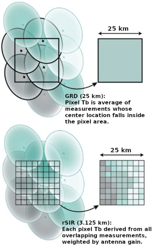
Figure 1. Low-vs. Enhanced-Resolution Concept; gridding techniques for GRD (top) and rSIR (bottom) [Credit (Brodzik and Long, 2018)].

The primary goals of this study are as follows:

1. Test correlation between SWE and CETB SSD to identify spatiotemporal patterns,

2. Assess the utility of CETB SSDs in improving the retrieval of SWE and other environmental variables that may contribute to spatiotemporal variability in SSD,

3. Enhance the accuracy of PMW SWE estimation for a heterogeneous snowpack and surface conditions.

2 Materials and methods

2.1 Data collection

2.1.1 In-situ SWE data

Daily ground observations of SWE were obtained from the Natural Resources Conservation Service (NRCS) SNOpack TELemetry (SNOTEL) Network, available on the United States Department of Agriculture (USDA) website (USDA, https://www.nrcs.usda.gov/wps/portal/wcc/home/snowClimateMonitoring/, last access: 15 September 2024) (SNOTEL, 2024). SNOTEL stations provide automated measurements of SWE, SD, Precipitation, Air Temperature (AirTemp), and other environmental parameters at high-elevation sites. The network operates continuously, offering hourly measurements, making it ideal for monitoring snowpack changes over time. SNOTEL SWE is used for the Correlation Analysis in Section 2.3.1. The spatial distribution of the selected stations in the Western US is shown in Figure 2 and Table 1. The time frame from January to December of the years 2000–2005 represents a temporal window with daily SNOTEL and PMW observations, as well as other required data mentioned in the following sections. This specific window was chosen arbitrarily. Future work will extend this over a longer period of record and over more sites.

Figure 2

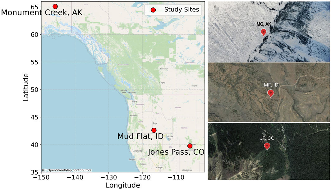
Figure 2. SNOTEL study sites and their respective landscapes, showing different environments in AK, ID, and CO. The right panel displays site landscapes: the top shows MC, AK (Tundra/Boreal Forest Snowpack); the middle shows MF, ID (Prairie); and the bottom shows JP, CO (Boreal Forest Snowpack, Rocky Mountain National Park) (Liston and Sturm, 2021).

Table 1

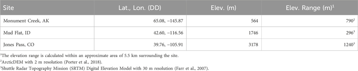
Table 1. Site information.

2.1.2 PMW Calibrated Enhanced-Resolution Brightness Temperatures (CETBs)

The Enhanced-resolution PMW data (CETB) uses the radiometer version of the Scatterometer Image Reconstruction (rSIR) method to generate enhanced-resolution data (Long and Brodzik, 2015; Brodzik et al., 2016). The CETB dataset also includes coarse resolution or GRD pixels produced using the “drop-in-the-bucket” method at a 25 km spatial resolution, which provides smoother data with lower noise and are most comparable to legacy PMW datasets (also at 25 km). The rSIR pixels, which may have greater noise, offer enhanced resolutions nested at 6.25 km (16 times finer at 18/19 GHz) and 3.125 km (64 times finer at 36/37 GHz) resolutions (Long and Brodzik, 2015; Brodzik and Long, 2018) (see Figure 1). There are three types of CETB spatial statistics: 1) GRD standard deviation (SDGRD), which represents the standard deviation of measurements contributing to each pixel in the GRD dataset, 2) rSIR standard deviation, provided with the CETB data for each rSIR pixel, which reflects the standard deviation of the differences between measured $T_b$ and their forward projections during reconstruction. This value is generally small and consistent, except in regions with large spatial gradients, indicating how well the reconstructed $T_b$ field matches the measurements, and 3) CETB SSDs, calculated from the enhanced-resolution $T_b$ data (64 rSIR pixels) for use in this paper, which represents the spatial variability within 64 rSIR pixels corresponding to a single GRD pixel. CETB SSDs correlate strongly with SDGRD and are sensitive to sub-pixel heterogeneity, making them valuable indicators of spatial variability and change. This study uses daily 37 GHz CETB version one observations from SSM/I radiometer aboard the F13 satellite, at both 25 km and 3.125 km spatial resolutions between 2000 and 2005.

The CETB data, including those used in this study, are freely available for download from the National Snow and Ice Data Center (NSIDC) at https://nsidc.org/data/nsidc-0630/versions/1. The dataset provides enhanced-resolution $T_b$ measurements, which are essential for snow, ice, and environmental-related studies.

2.1.3 NASA GLDAS Noah version 2 data products

NASA’s Global Land Data Assimilation System (GLDAS) Noah data, including SWE, Soil Moisture (SM), AirTemp, Surface Temperature (SurfaceTempt), Albedo, Downward Short-wave Radiation Flux (RadiationFlux), SD, Snowmelt, and Wind Speed (WS) were utilized. These data are available at 3-h intervals, and the daily mean values were computed across the 3-h intervals using Google Earth Engine (GEE) to create a time series for each location. The spatial resolution of the data is 0.25 × 0.25, approximately equivalent to 27.75 km × 27.75 km at the equator (Rodell et al., 2004; Beaudoing and Rodell, 2020). This resolution was downscaled to approximately 25 km using aggregation methods in GEE, which closely aligns with the 25 km resolution typical of legacy PMW data and CETB GRD, facilitating direct comparisons and integrations of datasets from different sources. The downscaling was achieved by applying a mean reducer over each 25 km grid cell, computing the average value of all pixels within a 25 km radius around each SNOTEL site. Currently, the mean value of all pixels within the 25 km grid cell is computed using a simple unweighted average, meaning each pixel contributes equally to the mean, regardless of the percentage of its area that overlaps with the 25 km grid cell. The inclusion of SM, AirTemp, Albedo, RadiationFlux, SD, Snowmelt, and WS, along with SWE, is pivotal in exploring how these factors interact with CETBs and their SSD across the terrain using ML methods. GLDAS SWE is used for the Feature Importance Analysis in Section 3.2. Each variable provides critical information about land surface conditions as shown in Table 2 (Rodell et al., 2004). These variables were selected to help understand and explain the key drivers behind CETB SSD variability and its relationship with SWE. Each of these environmental factors can influence snowpack dynamics, land surface conditions, and microwave emissions, making them critical for identifying the processes that contribute to SSD variations. The GLDAS data products, including these variables, are available for download through NASA’s Goddard Earth Sciences Data and Information Services Center (GES DISC) at https://ldas.gsfc.nasa.gov/gldas (last accessed: 3 October 2024).

Table 2

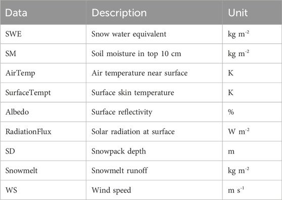
Table 2. GLDAS variables description.

2.1.4 MODIS NDVI

The Normalized Difference Vegetation Index (NDVI) dataset from the Moderate Resolution Imaging Spectroradiometer (MODIS) sensor aboard the Terra satellite was used to analyze vegetation trends at the three study sites (Didan, 2015). The MODIS NDVI data is available at a native spatial resolution of 500 m, with data processed between 2000 and 2005. The GEE platform was used to extract daily NDVI values over the study period. To facilitate comparison with other datasets, the NDVI data was aggregated to approximately 25 km resolution, computing the average NDVI within a 25 km radius around each SNOTEL site. NDVI was included in this study to assess its potential influence on CETB SSD variability, as vegetation cover can impact microwave signal scattering and attenuation. The MODIS NDVI data from the Terra satellite can be accessed from NASA’s EarthData portal at https://earthdata.nasa.gov/, and then processed using GEE.

2.2 Study area and site selection reasoning

The Western U.S., with its crucial snowpack, presents an ideal study area with the availability of snow field measurements. The region’s diverse climate, topography, vegetation, and snow properties pose challenges for accurate remotely-sensed SWE estimations. The initial study area focuses on a suite of watersheds in the Western US with comprehensive data availability for the period of record, representing a variety of environments. These areas are used to test the hypothesis and validate its robustness across different conditions, with an initial focus on three SNOTEL sites: Monument Creek (MC) in Alaska, Mud Flat (MF) in Idaho, and Jones Pass (JP) in Colorado (Table 1; Figure 2).

The selection of these initial sites, based on their environmental complexity in relation to SWE estimation, serves as a foundation for a broader analysis (Figure 2). JP in Colorado is the most complex due to its complex topography and rugged mountainous terrain. This creates diverse microclimates, leading to complex interactions between snowpack and other environmental variables. The mid-latitude location further experiences intense solar radiation and significant snowpack fluctuations, making it a challenging region for snow and SWE estimation models, as multiple variables must be taken into account. MC, AK, although experiencing long snow seasons, presents less complexity due to its relatively homogeneous landscape and sparse vegetation. In MC, snowpack and SWE dynamics can be the primary drivers of seasonal variability in CETBs, and fewer environmental variables, like tundra vegetation, influence snowpack dynamics. MF in Idaho, characterized by less complex topography and lower vegetation coverage (prairie land cover (Dewitz, 2023)), was chosen as a simpler site to help isolate the impact of horizontal dynamics on the ground (red arrow in Figure 3) for more accurate SSD_SWE analysis, in contrast to the more complex Alaskan and Colorado sites, which introduce additional variables (topography and vegetation complexities) into the analysis (Figure 3). MF has a shorter, more variable snow season and shallower snowpack compared to the other sites. Figure 3 shows how surface heterogeneity (red arrow direction) can affect microwave signals, impacting signals of interest for snowpack estimations (blue arrow direction). Including different sites in the analysis will ensure a thorough understanding of the correlation between SWE and SSD in diverse snow landscapes.

Figure 3

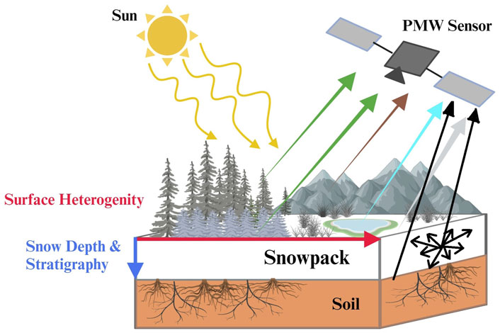
Figure 3. Horizontal (Red arrow) and Vertical (Blue arrow) Complexity Schematic for Snowpack RS Using PMW Sensors (Created in BioRender. Boueshagh, M. (2025) BioRender.com/l60q566). This approximate schematic illustrates how PMW RS operates (Canada, 2015) while highlighting horizontal and vertical complexities. Surface heterogeneity, such as vegetation, terrain, and water bodies, affects microwave signal reflection and scattering, representing horizontal complexity. Vertical complexity arises from snowpack characteristics like depth and stratification, influencing microwave emissions. The sun’s influence, which affects surface temperature and indirectly impacts $T_b$, is also depicted, contributing to the signal detected by the PMW sensor. The black arrows represent emissions from the soil surface and volume scattering within the snowpack.

2.3 Methods

2.3.1 SWE and CETB SSD correlation analysis

PMW RS detects naturally emitted microwave radiation from the Earth’s surface and atmosphere. These emissions, measured as $T_b$, depend on the physical temperature and the emissivity of the surface materials ($T_b\approx ϵ\cdot T_s$, $ϵ$: emissivity, and $T_s$: surface physical temperature). PMW radiometers capture microwave radiation emitted from snow and underlying soil and estimate SWE, particularly effective in dry snowpack conditions (Chang et al., 1976; Chang et al., 1987).

For a simpler region, factors such as surface roughness and vegetation height or density are present but have minimal impact on SWE estimation due to the relatively uniform surface and sparse vegetation. Thus, we assume the microwave signal represented as Equation 1:

$P_{\text{microwave,\hspace{0.17em}simple}}=f\left(T_s,ϵ,S\right)(1)$

In contrast, for a more complex region, the microwave signal is influenced by additional factors as shown in Equation 2:

$P_{\text{microwave,\hspace{0.17em}complex}}=f\left(T_s,ϵ,S,z_0,h\right)(2)$

Where:

• $P_{\text{microwave,\hspace{0.17em}simple}}$ is the microwave signal power for the simpler site.

• $P_{\text{microwave,\hspace{0.17em}complex}}$ is the microwave signal power for the more complex site.

• $T_s$ is the SurfaceTempt, which includes contributions from both the soil and the snow depending on the snowpack’s thickness and the penetration depth of the microwave signal.

• $ϵ$ is the surface emissivity.

• $S$ represents the snow properties (e.g., SD, SWE, grain size, etc.).

• $z_0$ is the surface roughness of the snow surface or soil surface, depending on the presence and thickness of the snowpack.

• $h$ represents the vegetation height or density.

By isolating the impact of snow properties in a simpler area (blue arrow in Figure 3), and assuming that temperature, emissivity, surface roughness, and vegetation height or density remain constant during the winter, we can express the change in microwave signal as being primarily due to snow and its variations as shown in Equation 3:

$\mathrm{\Delta }{P}_{\text{microwave}}=f\left(S\right)(3)$

This isolation allows us to better understand the specific impact of snow properties on microwave signals without the additional variables present in more complex sites. To address the large footprint issue of legacy PMW data pertinent to SWE estimation, CETB data provides significant improvements over legacy data in distinguishing finer spatial patterns, which is especially useful in heterogeneous landscapes. The CETB data, with its fine spatial resolution and twice-daily (morning and evening overpasses) temporal resolution, improves the accuracy of snowpack analysis in heterogeneous landscapes (Long and Brodzik, 2015; Brodzik and Long, 2018). Importantly, CETB allows for calculating the SSD using multiple higher-resolution pixels (Figures 1, 4; Equation 4), which was not previously possible with legacy PMW data. SSD is a measure of variability and spread of the $T_b$ values, providing insights into the variability of snowpack properties both over the surface and in-depth in the observed area. We define the SSD value as follows:

${\text{SSD}}_{\mathit{rSIR}}\left(K\right)=\sqrt{\frac{{\sum }_{n=1}^{64}{\left(T{b}_n\left(K\right)-\mu \left(K\right)\right)}^2}{N}}(4)$

where $\mu$ refers to the mean of $T_b$, K represents the unit $[Kelvin]$, and N is the number of pixels containing $T_b$ values (64 rSIR pixels with 3.125 km resolution or an 8 × 8 window corresponding to a GRD pixel), and n represents the index of each individual rSIR pixel, with n ranging from 1 to 64.

Figure 4

Figure 4. CETBs for the Morning Overpass on 18 February 2003, at Monument Creek, AK. This figure displays the spatial variability of Tbs from the CETB dataset. The red square outlines the GRD pixel, which serves as an envelope for the higher-resolution CETB pixels (3.125 km). The red box and line on the color bar indicate the corresponding GRD pixel and Tb value of the GRD pixel (in K), respectively.

The experiment aims to assess how the SSD of rSIR CETBs can enhance SWE estimation, particularly in complex mountainous regions. The hypothesis evaluation involves comparing and correlating (Pearson correlation) daily SNOTEL and PMW-based SWE with morning overpasses of SSD with 3.125 km spatial resolution within GRD pixels and Equation 4 for the sites of interest. The comparison reveals notable patterns and correlations, which are further explored and discussed in the following sections (Sections 3 and 4). By focusing on the morning (colder) passes, this approach minimizes underestimation caused by warmer temperatures later in the day, which may have caused melt (Chang et al., 1987; Armstrong and Brodzik, 2002). Furthermore, the vertical channel of CETB SSD is preferred due to:

• Sensitivity of Vertical polarization (V-pol) to Moisture: V-pol is highly sensitive to the liquid water in both the soil and the snowpack (Mätzler, 1994; Njoku and Kong, 1977; Kim and Van Zyl, 2009; Temimi et al., 2014; Picard et al., 2022), particularly to the amount of water contained within the snowpack, known as SWE. The microwave radiation interacts with the liquid water and ice within the snowpack, and the V-pol signal is influenced by factors such as SD, density, and water content. This sensitivity allows V-pol to effectively capture variations in water content.

• Surface Inhomogeneity: V-pol is less influenced by surface heterogeneity, such as variations in vegetation, soil type, and surface roughness, compared to horizontal polarization (H-pol). V-pol passes through the snow surface with minimal reflection or scattering, allowing most of the microwave energy to be transmitted. This efficient transmission results in higher $T_b$ values at V-pol, as less energy is lost during the interaction with the snowpack surface (Markus et al., 2005; Picard et al., 2022). Additionally, the efficient transmission of V-pol signals is associated with a higher saturation limit for SWE compared to H-pol, offering an advantage in estimating deeper snowpack. Furthermore, V-pol exhibits greater sensitivity to snow depth than H-pol channels (Takala et al., 2011; Yang et al., 2020; 2022). By analyzing the standard deviations of V-pol $T_b$, the algorithm can better capture variations in SD across different pixels while minimizing the influence of surface features that primarily impact H-pol.

• Combining H-pol and V-pol: By integrating the strengths of both H-pol and V-pol, the algorithm benefits from H-pol’s ability to detect snow structure and surface roughness, and V-pol’s sensitivity to moisture content and reduced impact from surface heterogeneity. This combination, along with the analysis of V-pol $T_b$ standard deviations, allows for a more comprehensive characterization of SD heterogeneity.

For correlation analysis, to ensure consistent comparisons in terms of spatial resolution with CETB SSDs, we also estimated the PMW-derived SWE using the CETB GRD pixel with 25 km spatial resolution and the modified Chang algorithm (Chang et al., 1987; Armstrong and Brodzik, 2001). This algorithm estimates SWE by multiplying SD, derived from a regression of $T_b$ gradients, by an assumed constant value for snow density (0.30 g/cm³) (Chang et al., 1987). Specifically, the gradient refers to the difference between $T_b$ at two frequencies, typically 19 GHz and 37 GHz. This approach, based on a linear regression between SMMR $T_b$ gradients and SWE, typically assumes a snow grain size of 0.3 mm and a density of 300 kg/m3 (Chang et al., 1987; Liang and Wang, 2020). In this study, we used a modified version developed by (Armstrong and Brodzik, 2001), which incorporates a bias correction to adapt the formula for use with SSM/I data (using $T_b$19H instead of $T_b$18H) (Equation 5).

$SWE\left(mm\right)=4.8\times \left(T_{b,19\text{H}}-T_{b,37\text{H}}-5\right)(5)$

Following established practices, we implemented thresholds to ensure the accuracy and physical relevance of the results. Specifically, SD values below 2.5 cm, corresponding to PMW-derived SWE values less than 7.5 mm, were thresholded and set to zero. This is due to the limitations of PMW data in reliably detecting shallow snowpacks, as the microwave signal sensitivity diminishes at such low depths (Tanniru and Ramsankaran, 2023), and negative values are not physically meaningful in snowpack studies and are likely artifacts of noise or algorithm limitations.

2.3.2 Feature importance analysis using ML

New PMW CETB data could provide a valuable proxy for SWE through statistics such as the SSD. While the calculated correlations and observed patterns between SNOTEL or PMW-derived SWE and CETB SSDs, discussed in Sections 3, 4 (Table 3; Figure 7), suggest a relationship, correlation alone does not imply causation. It is therefore essential to investigate the underlying components that may influence SSDs. By examining these factors, we can better understand whether the observed correlation is primarily driven by snow-related variables or other environmental factors. This deeper understanding is crucial for validating the use of SSDs as a proxy for SWE estimation while acknowledging and addressing potential confounding influences.

Table 3

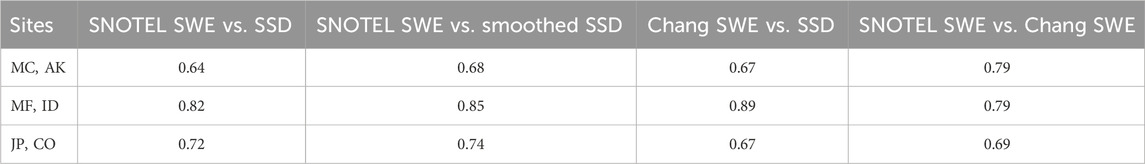
Table 3. Pearson correlation coefficient (r) results.

This study employs 4 ML techniques (Linear Regression (LR), RF, Gradient Boosting (GBoost), and Extreme Gradient Boosting (XGBoost)) to explore the key factors influencing SSDs at each site, aiming to disentangle their contributions using a workflow that involves data preprocessing, outlier removal, training, cross-validation (CV), and interpretability using feature importance and SHapley Additive exPlanations (SHAP) analysis. By identifying the drivers of SSD, we can test and explain the hypothesis that the correlation between SNOTEL or PMW-derived SWE and CETB SSDs is due to snow-related variables and/or maybe other environmental variables. To achieve the study’s objectives, we adopted a modeling approach where SSD serves as the target variable (dependent variable), and various environmental factors are treated as predictor variables (independent variables). Our goal is to evaluate whether CETB SSD can serve as a useful proxy for SWE by identifying the key drivers of CETB SSD variability across different geographic and climatic regions. Setting CETB SSD as the target variable allows us to assess how strongly SWE and other environmental factors (e.g., AirTemp, SM, albedo, etc.) contribute to CETB SSD observed variability. This step is crucial in determining whether CETB SSD contains a reliable and consistent SWE signal that could be leveraged for future SWE estimation. Our study first aims to establish whether CETB SSD responds to SWE variations before integrating it into direct SWE estimation models. This analysis serves as a diagnostic step to justify the inclusion of CETB SSD in future SWE retrieval algorithms. The key difference between regression (the task for feature importance analysis) and correlation (the task for identifying associations between SSDs and SNOTEL or PMW-derived SWE) lies in their purpose and interpretation. Regression aims to model the relationship between a dependent variable and one or more independent variables to understand the influence of these variables. In contrast, correlation measures the strength and direction of the linear relationship between two variables but does not imply a cause-and-effect relationship or allow for predictions. While correlation quantifies how two variables change together, regression (the ML approach adopted in this research) focuses on how one variable can be predicted based on the values of another. The methodology involves the following key steps (Figure 5).

Figure 5

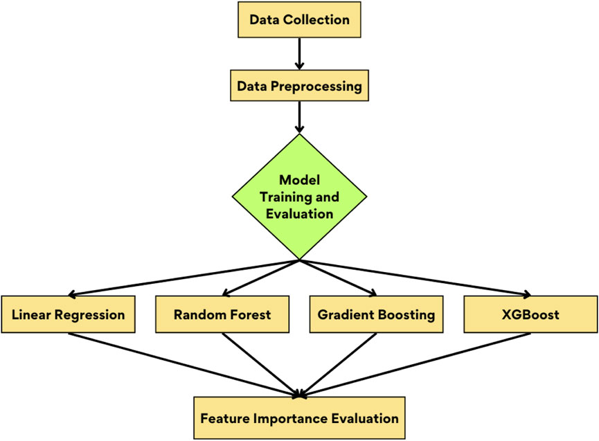
Figure 5. Methodology for feature importance evaluation and exploration of key CETB SSD drivers.

2.3.2.1 Data preparation for feature importance analysis

The dataset comprises daily values of CETB SSDs (target variable), and GLDAS SWE, SM, AirTemp, SurfaceTempt, Albedo, RadiationFlux, SD, Snowmelt, and WS, as well as MODIS NDVI (predictor variables) for 2000-2005 (Table 2). Here, we use GLDAS SWE, instead of SNOTEL SWE or Chang SWE, to do feature importance analysis because GLDAS SWE is more consistent with other GLDAS variables. The purpose of this analysis is to identify the most important drivers of CETB SSD variability, particularly focusing on snow-related variables such as SWE. While SNOTEL SWE offers accurate ground-based data, its spatial resolution is limited to specific point locations, which may not capture spatial or regional variability. Chang SWE, derived from PMW data, is prone to biases, outliers, and inconsistencies, especially in areas with dense vegetation, complex topography, or wet snow conditions (Saberi et al., 2020). GLDAS SWE, by integrating satellite and in situ data, provides a more consistent dataset across varied landscapes.

The comparison between SNOTEL SWE and GLDAS SWE across all three sites reveals important biases and discrepancies that can influence the interpretation of CETB SSD variability with respect to SWE (Figure 6). At MC, both datasets align relatively well in capturing seasonal accumulation and melt patterns, although GLDAS SWE tends to underestimate peak SWE values compared to SNOTEL, particularly during 2001 and 2004. In JP, the mismatch is more pronounced, with GLDAS SWE significantly underestimating SWE throughout the period, capturing only minimal snowpack variability compared to the sharp peaks in SNOTEL. This suggests that GLDAS’s lower resolution and large negative precipitation biases are more pronounced in regions with complex terrain and higher elevation, where modeled SWE struggles to capture local snowpack dynamics (Han et al., 2020). In contrast, MF shows better agreement between the two datasets, with GLDAS SWE closely following the accumulation and melt trends observed in SNOTEL, possibly due to less spatial variability at the 25 km scale. However, small discrepancies remain during peak periods, likely reflecting differences in how GLDAS and SNOTEL capture melt events and transient snowpack conditions in this semi-arid region. The cross-comparison of SNOTEL and GLDAS SWE across these three sites highlights the strengths and limitations of each dataset in different environmental contexts. While SNOTEL SWE provides reliable ground-based measurements, its point-based observations may not capture regional variability, particularly in areas like MF, where spatial snow dynamics can vary significantly. GLDAS SWE, on the other hand, offers better spatial coverage but suffers from modeling biases (Han et al., 2020), as evidenced by its consistent underestimation of SWE in JP and a tendency toward smoother seasonal variations in SWE at MC. These limitations are critical, as GLDAS’s underestimation of SWE may weaken the observed relationship between SWE and SSD variability, underrepresenting the snowpack’s role in CETB SSD signals.

Figure 6

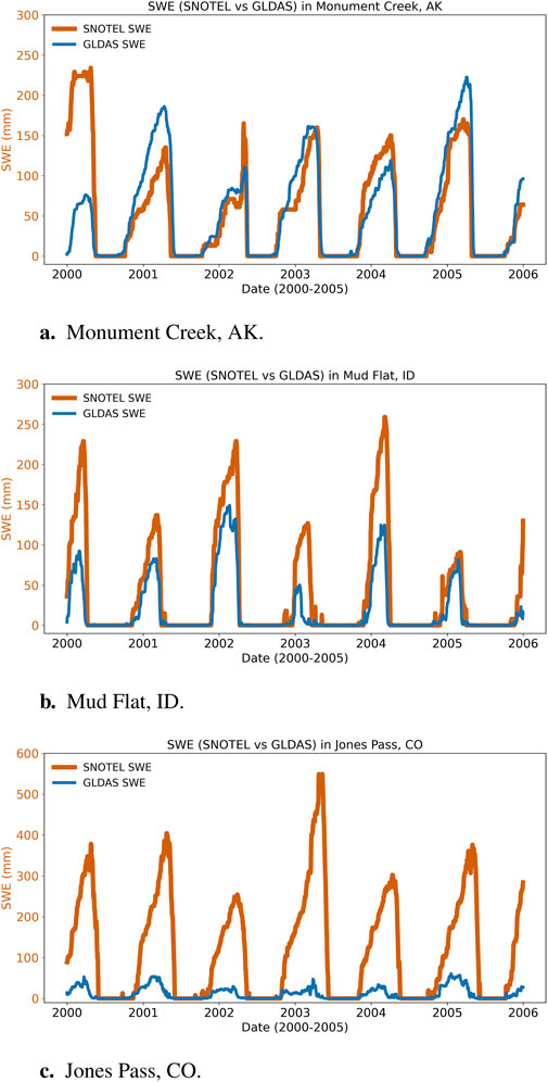
Figure 6. Comparison of SWE (SNOTEL & GLDAS) for (A) Monument creek, AK, (B) Mud Flat, ID, and (C) Jones pass, CO (2000-2005).

2.3.2.2 Data splitting, standardization, and outlier removal

• Outlier Removal: We first examined the time series of CETB SSD in Figure 7 and identified sites with potential outliers in the data. Outliers were then detected and removed using the Interquartile Range (IQR) method, filtering out data points that fell outside 1.5 times the IQR from the first and third quartiles. For MC in AK and JP in CO, outlier removal was applied across all models to ensure consistency and prevent extreme values from influencing the analysis. Although the IQR filter was also applied to MF in ID, no significant outliers were identified at this site.

• Train-Test Split: The cleaned dataset was divided into training and testing sets using an 80%–20% split. This split is commonly used in ML to ensure the model has enough data to learn from during training (80%) while still retaining a sufficient portion (20%) for testing on unseen data, helping to evaluate model performance and avoid overfitting.

• Standardization: Features were standardized to have a mean of 0 and a standard deviation of 1. This process is crucial for models like LR, which are sensitive to the scale of input data, and helps ensure that each feature is treated equally during the training process.

Figure 7

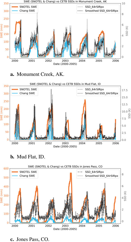
Figure 7. Comparison of SWE and SSD time series (2000-2005) for (A) MC, AK, (B) MF, ID, and (C) JP, CO. The correlations between CETB SSD and both SNOTEL SWE and Chang algorithm SWE (as presented in Table 3) are illustrated, highlighting the relationship between snowpack variability and SWE estimations at each site. At JP, discrepancies between SNOTEL SWE and PMW-derived SWE are particularly noticeable during peak snow periods, suggesting limitations in the Chang algorithm’s performance in more complex snowpack environments. In contrast, at MF, the simpler snowpack characteristics result in a stronger and more consistent association across the entire time series, demonstrating a reliable relationship between SSDs and SWE in less complex terrains.

2.3.2.3 Model training and evaluation

• ML Models: The following ML models were employed to assess their ability to predict CETB SSDs based on the selected predictors:

• LR: LR models the relationship between the predictor variables and the target variable by fitting a multiple linear regression. It is sensitive to outliers. The model minimizes the sum of squared residuals and assumes a linear relationship between the predictors and the target. LR provides interpretable results through its coefficients, indicating the strength and direction of relationships (Montgomery et al., 2021).

• RF Regressor: RF is an ensemble learning method based on decision trees. It constructs multiple decision trees using random subsets of the data and features. The final prediction is the average of the individual tree outputs, making RF robust to overfitting and outliers. To ensure the trees were effectively pruned and the model generalized well, hyperparameter tuning was performed using CV mentioned in the next paragraphs of this section. Additionally, RF provides feature importance scores by evaluating the contribution of each feature to the decision-making process (Breiman, 2001).

• GBoost Regressor: GBoost is an ensemble technique that sequentially builds decision trees, with each new tree correcting the errors of the previous ones. This iterative process optimizes a loss function to improve predictions over time. GBoost captures complex relationships but is more sensitive to outliers compared to RF (Friedman, 2001).

• XGBoost Regressor: XGBoost is an optimized version of GBoost that incorporates regularization to prevent overfitting, making it robust and scalable. It sequentially builds trees to correct errors from the previous models and includes advanced features like missing value handling and parallelization for faster training (Chen and Guestrin, 2016).

• Hyperparameter Tuning: To optimize the performance of the tree-based models (RF, GBoost, and XGBoost), hyperparameter tuning was performed using Grid Search Cross-Validation (GridSearchCV). A grid search over predefined hyperparameters was conducted for each model. For RF, the number of estimators, maximum depth, minimum samples per split, and minimum samples per leaf were tuned. For GBoost and XGBoost, additional parameters such as the learning rate, number of estimators, maximum depth, and subsampling rate were included. GridSearchCV was used with a 3-fold CV to identify the best set of hyperparameters for each model and ensure that models were optimized for performance and generalization. Once the best parameters were identified, the models were trained using these optimal configurations for final predictions.

• CV and Training: Each model was trained on the standardized training data. A 5-fold CV was applied to evaluate model performance by splitting the data into five subsets. Each subset served as a validation set once, while the remaining subsets were used for training. This provided a more reliable measure of model performance and reduced overfitting.

• Prediction and Evaluation: The models made predictions on the testing set, and performance was evaluated using the following metrics:

• R-squared (R²): Also known as the coefficient of determination, measures the proportion of variance in the target variable that is explained by the model. Higher R² values indicate better model performance.

• Root Mean Squared Error (RMSE): Measures the square root of the average squared differences between the predicted and actual values. RMSE provides an indication of the model’s prediction error in the same unit as the original data ([K]). Lower RMSE values indicate more accurate predictions.

2.3.2.4 Feature importance and SHAP analysis

• For Tree-Based Models (RF, GBoost, XGBoost): Feature importance scores were extracted from the tree-based models to quantify each feature’s contribution to the prediction of CETB SSDs and provide insights into the relationships between predictors and CETB SSDs. Feature importance quantifies the increase in model error when a specific feature is removed or its values are randomized, helping to highlight which variables significantly influence SSDs and validate the role of snow-related factors in the observed correlation with SWE. Additionally, SHAP analysis was employed to provide a more detailed interpretation of each feature’s impact. SHAP values explain how much each feature contributes to increasing or decreasing the predicted value of SSDs for each individual prediction. The SHAP analysis offers global insights into feature importance across the dataset and local explanations for individual predictions (Lundberg, 2017; Li, 2022; Aydin and Iban, 2023). SHAP values are especially helpful in understanding the complex interactions in models like XGBoost and RF, which may not be as interpretable through traditional feature importance alone. By assigning Shapley values, SHAP ensures that the contribution of each feature is fairly allocated, making it clear how snow-related factors like SWE drive the variability in CETB SSDs (Lundberg, 2017; Li, 2022; Aydin and Iban, 2023). Using a pre-trained ML model and a set of input variables, SHAP utilizes an explanation model to determine the individual contribution of each variable to the behavior of the model (Liu et al., 2022). In this study, we used the Python SHAP library to assess the importance of features.

In SHAP summary plots (Section 3.2), each element provides insight into how features contribute to model predictions. The dots represent individual data points, and their position along the x-axis shows the SHAP value, indicating how much a feature pushes the prediction higher (positive SHAP value) or lower (negative SHAP value). The color of the dots corresponds to feature values, with red representing higher values and blue indicating lower values. This color gradient helps reveal how feature values influence predictions. Dots are vertically aligned for each feature, and features are ordered by their mean absolute SHAP value, with the most important features at the top. A wider vertical spread of dots means that the feature’s impact on predictions varies more across data points. Dense clusters of dots indicate many data points with similar SHAP values. The range of SHAP values along the x-axis shows the degree to which each feature can affect predictions.

• For LR: In LR, feature importance is assessed through the magnitude of the model’s coefficients. Features with larger absolute coefficients have a stronger influence on the prediction, while the sign of the coefficient indicates whether the feature has a positive or negative relationship with SSDs. This provides a straightforward way to interpret the linear relationships between the predictors and the target. While the coefficients from LR give insights into linear relationships, SHAP analysis for tree-based models provides complementary non-linear insights, offering a comprehensive understanding of the factors influencing CETB SSDs.

3 Results

3.1 Hypothesis analysis and correlation results

To test the hypothesis, linear correlations (Pearson correlation/“r”) between SWE and CETB SSDs were computed. The correlations (as presented in Table 3), along with the robust associations observed across different periods and sites (as shown in Figure 7), reveal strong relationships. These findings suggest that CETB SSDs could serve as a valuable proxy for enhancing PMW SWE estimations, particularly in capturing the temporal and spatial heterogeneity of snowpack. The analysis implies that examining the variability in $T_b$ across multiple pixels can effectively capture the spatial heterogeneity of SD and terrain, leading to more accurate SWE estimates. The robustness of these results across sites and periods underscores their reliability. This insight indicates that integrating CETB SSDs into existing PMW-based SWE retrieval algorithms could improve their performance by addressing both the temporal and spatial variability inherent in snowpack characteristics. Table 3 summarizes the Pearson correlation coefficients (r) between SWE values from SNOTEL data and the Chang algorithm, and SSDs at each of the three study sites. The correlation analysis quantifies the strength of the relationship between these variables, showing how SSDs can enhance the interpretation of snowpack conditions.

Noise and outliers in PMW time series can impact forecasting. To address this, we smoothed the SSD time series using a median filter, which enhanced correlation, particularly in low or no-SWE conditions, while preserving critical details (see Table 3; Figure 7). After careful trial and error, considering noise levels, feature preservation, data resolution, and computational efficiency, a uniform window size of 13 days was chosen across the sites, which also corresponds to the temporal scale of synoptic events (Salas et al., 2022). The median filter was applied over a 13-day sliding window to the SSD values. This window size effectively reduces noise and highlights meaningful snowpack patterns without oversimplifying the data. This approach ensured that fine-scale details were retained, allowing for the detection of SSD variations in minimal snow conditions while considering gaps in PMW data at lower latitudes. As shown in Figure 7, we compared unsmoothed and smoothed data, which confirmed that the key relationships between CETB SSDs and SWE remained consistent. This demonstrates that the observed correlations are not solely artifacts of the smoothing process. We recognize, however, that smoothing can sometimes introduce artificially high correlations.

Figure 7 illustrates the comparison of the SWE time series derived from the SNOTEL and the Chang algorithm, along with CETB SSDs across the tested sites. The time series analysis reveals distinct correlations between SSDs and SWE at each site, highlighting the relationship between SSD and snowpack variability. While SNOTEL SWE serves as the ground truth, Chang SWE provides satellite-based estimates, and SSDs reflect spatial variability in $T_b$ across the sites. Notable differences in SWE values occur at each site, demonstrating how CETB SSDs complement both SNOTEL and PMW-derived SWE in capturing snowpack dynamics. The associations between smoothed SSDs and SNOTEL SWE further indicate the importance of noise reduction in improving the robustness of SWE estimations.

1. MC, AK: The moderate correlations between SNOTEL SWE and SSDs $(r=0.64)$ suggest that SSDs capture key aspects of snowpack heterogeneity affecting SWE estimations (see Figure 7A; Table 3). Smoothing the SSD time series increases the correlation $(r=0.68)$, underlining the value of noise reduction. The slightly stronger correlation between Chang SWE and SSDs $(r=0.67)$ further confirms the potential of SSDs to improve PMW-based SWE estimates. The high agreement between SNOTEL SWE and Chang SWE $(r=0.79)$ reflects a good alignment between ground-based and satellite-derived estimates, though further refinement is necessary for more complex snowpack features, such as ice layers or varying snow density. MC has a long-lasting snowpack with terrain that is less complex than JP but more complex than MF. The snowpack at MC may be more homogeneous in terms of snow properties (e.g., SD and density), leading to less variability in the microwave signal and, thus, lower SSD values.

2. MF, ID: In this region, strong correlations are observed between SNOTEL SWE and SSDs $(r=0.82)$, suggesting that SSDs effectively capture snowpack variability in what is generally considered a simpler terrain (see Figure 7B; Table 3). The correlation improves further when smoothing SSDs $(r=0.85)$, reinforcing the importance of filtering noise for SWE estimation accuracy. The high correlation between Chang SWE and SSDs $(r=0.89)$ highlights the ability of SSDs to reliably estimate SWE, likely due to a strong alignment between the snowpack characteristics at MF and the assumptions of the Chang algorithm. The correlation between SNOTEL SWE and Chang SWE $(r=0.79)$ also confirms the reliability of satellite-derived SWE estimates in this region. Despite the simplicity of the terrain, variability in snowpack conditions may arise due to solar radiation, wind redistribution, and subtle topographical influences, which could lead to higher values of SSDs as snowpack varies across the site.

3. JP, CO: Moderately strong correlations between SNOTEL SWE and SSDs $(r=0.72)$ reflect snowpack variability at JP (see Figure 7C; Table 3). Smoothing SSDs improves the alignment with SNOTEL SWE $(r=0.74)$, indicating the benefit of noise reduction. The time series shows good agreement between SNOTEL SWE and SSDs, though discrepancies between SNOTEL and Chang SWE occur during peak SWE periods. The correlation between Chang SWE and SSDs $(r=0.67)$ suggests SSDs can complement PMW-derived SWE estimates, particularly in complex environments like JP, where vegetation coverage and algorithm assumptions may lead to under- or overestimation during peak SWE.

Despite the complex terrain, SSD values at JP are slightly lower than those at MC and significantly lower than those at MF. Although JP has the largest SWE values, the snowpack may be thicker and more uniform, leading to less spatial variability in the microwave signal. Forest coverage at JP may also provide shade, reducing the snowpack’s exposure to solar radiation and wind redistribution, which would otherwise introduce variability. The dense forest and vegetation cover likely attenuate the microwave signal, making it less sensitive to snowpack variability. This attenuation may explain the lower SSD values, as the microwave sensor struggles to detect subtle changes in snow properties. The steep and rugged terrain at JP causes shadowing effects and localized variations in the snowpack, complicating the interpretation of microwave signals. These factors contribute to the lower SSD values. Finally, due to orbital limitations, PMW data at lower latitudes, such as those near JP, may have spatial or temporal gaps, with the frequency of missed observations increasing with proximity to the equator. These gaps may reduce the number of CETB observations per day over the surface and limit the ability to detect snowpack variability effectively within a GRD pixel (an envelope of 64 rSIR pixels), contributing to the lower SSD values at JP.

To assess the statistical significance of the observed correlation between SNOTEL SWE and CETB SSD, we utilized Monte Carlo simulations alongside bootstrap resampling methods. The results confirm that the correlations are statistically significant and are detailed in the Supplementary Materials. Based on observations from Figure 7, an increasing SSD trend may indicate a spatially variable snowpack and terrain, characterized by heterogeneity in SD, density, grain size, or structure across the observed area. This variability often results from factors such as uneven snowfall, wind redistribution, or partial melting. Such conditions necessitate careful consideration in SWE retrieval due to increased uncertainty in interpreting microwave signals. Conversely, a decrease in the SSD trend may suggest reduced snow variability or the diminishing presence of snow. Seasonal variations in SSD reflect the dynamic nature of the snowpack: SSD may be lower during the early accumulation phase, increase as the snowpack becomes more heterogeneous during peak SWE, and then decline as SWE decreases later in the season when the snow cover becomes sparse or disappears entirely. The analysis of correlations and associations between SWE from SNOTEL, Chang algorithm SWE, and CETB SSDs across three sites highlights the strength of the relationship of SSDs in capturing snowpack variability and its impact on SWE estimates. It should be noted that in regions with deep snowpack, such as those observed near the peak accumulation periods in Figure 7, the PMW signal can experience saturation. This occurs because the emitted microwave signal becomes insensitive to additional increases in SD or density beyond a certain threshold (SWE_max $\approx$ 150–200 mm), causing an underestimation of SWE (Cho et al., 2023).

3.2 Feature importance results

The primary objective of this feature importance analysis using ML techniques is to identify the key drivers influencing the CETB SSDs and to understand their impact on the observed correlation between SSDs and SWE, and assess whether SSDs can improve PMW SWE estimates. To achieve this, we employed several ML models, including LR, RF, GBoost, and XGBoost. Each model provided insights into the importance of various environmental variables, including SWE, SM, AirTemp, NDVI, SurfaceTempt, Albedo, RadiationFlux, SD, Snowmelt, and WS. These models helped to elucidate how these factors contribute to the variability in CETB SSDs and their subsequent relationship with SWE.

The model performance comparison across the three sites-MC, MF, and JP-reveals that MC in AK consistently shows the highest predictive accuracy across all models, with RF and XGBoost achieving the best results, each with an R² of 0.89 and low RMSE values around 0.37 to 0.39 on test data (Table 4). In contrast, MF in ID demonstrates moderate performance, with XGBoost and RF yielding R² values between 0.73 and 0.74, but with higher RMSEs (0.97–0.98) on test data. JP, CO shows the weakest performance, with LR yielding the lowest R² of 0.44 and the highest MSE (0.51) on test data, while tree-based models perform slightly better but still struggle with predictive accuracy, with XGBoost achieving the highest R² of 0.63 and RMSE of 0.58 on test data. In general, the models predict CETB SSD variability most accurately at MC, AK, moderately at MF, ID, and least effectively at JP, CO, highlighting site-specific challenges in capturing variability. The ML model performance for predicting CETB SSD variability at the MC, AK site shows that tree-based models (RF, GBoost, and XGBoost) consistently outperform LR in both CV and test data (Table 4). LR, with an average R² of 0.72 and a test R² of 0.75, captures some relationships between predictors and the target but struggles with complex interactions. In contrast, RF, GBoost, and XGBoost achieved significantly better test R² values of 0.89, 0.88, and 0.89, respectively, and lower RMSE values, indicating their superior ability to capture non-linear relationships. Among these, RF showed the highest performance, closely followed by XGBoost. These results underscore the suitability of tree-based models for predicting CETB SSD variability.

Table 4

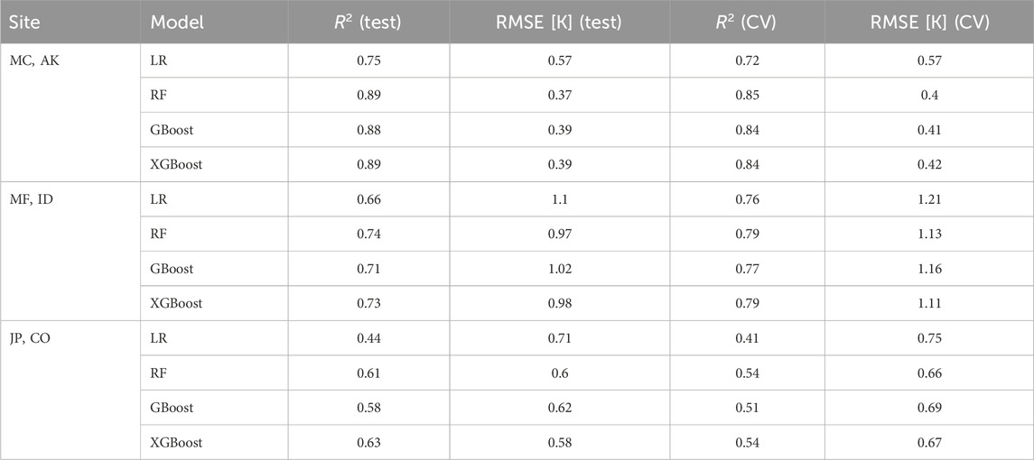
Table 4. Model performance on test data and CV for each site.

Feature importance and SHAP analysis provide further insights into variable contributions at MC, AK (Figures 8A, B). SWE emerged as the most influential predictor across all models, with significant importance in LR (1.08), RF (0.69), GBoost (0.69), and XGBoost (0.53). High SWE values were linked to higher SSD predictions, illustrating a strong relationship between SWE and SSD variability. Other variables, such as AirTemp, SM, and Albedo, also contributed notably, with SHAP analysis emphasizing their impact. Specifically, SM and AirTemp could influence depth hoar formation under cold, shallow snowpack, where large temperature gradients develop between the snow surface (affected by AirTemp) and the ground (influenced by SM), such as at MC. This increases microwave scattering and affects SSD, which can lead to overestimations of SD by algorithms like Chang, making the snowpack appear deeper (larger SWE values) than it actually is (see Figure 7). Energy exchange variables, such as Albedo and RadiationFlux, also played a role, though to a lesser extent.

Figure 8

Figure 8. (A) Feature importance, and (B) SHAP summary results for Monument Creek, AK. The dots in (B) represent individual data points, and their position along the x-axis shows the SHAP value, indicating how much a feature pushes the prediction higher (positive SHAP value) or lower (negative SHAP value). The color of the dots corresponds to feature values, with red representing higher values and blue indicating lower values. Dots are vertically aligned for each feature, and features are ordered by their mean absolute SHAP value, with the most important features at the top.

At the MF site, RF emerged as the best-performing model, with a test R² of 0.74 and the lowest RMSE (0.97) on test data, closely followed by XGBoost (R² = 0.73, RMSE = 0.98). GBoost, while slightly less accurate, still performed reasonably well (R² = 0.71, RMSE = 1.02). LR, despite decent CV results (R² = 0.76), underperformed on the test set (R² = 0.66, RMSE = 1.1) (Table 4). Feature importance for MF, ID confirmed SWE as the most significant variable, with high values driving SSD predictions upward (Figures 9A, B). In LR, SWE and SD were the most critical predictors, while SurfaceTempt and Albedo also played roles in snowmelt processes. For tree-based models, SWE, SM, and RadiationFlux were key, reflecting their ability to capture interactions between moisture, energy fluxes, and SSD variability. SM was influential in RF and XGBoost models, pushing SSD predictions higher when SM values were elevated.

Figure 9

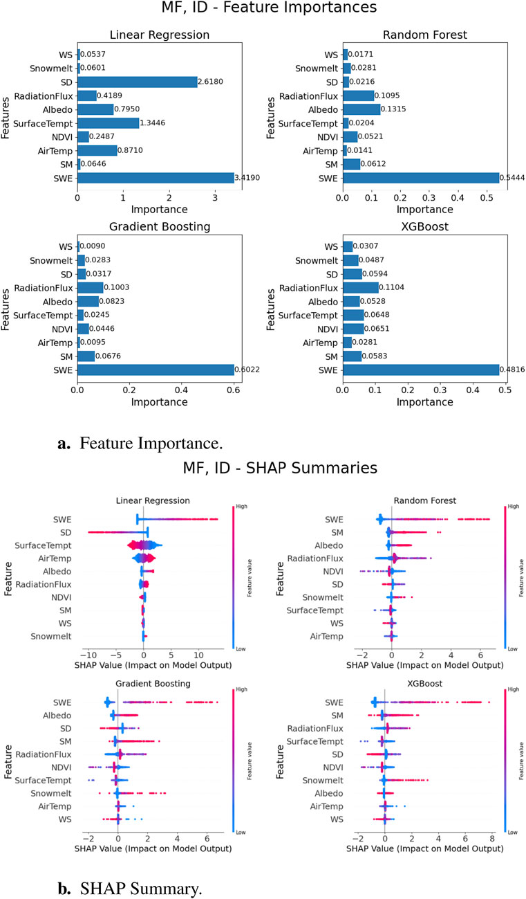
Figure 9. (A) Feature importance, and (B) SHAP summary results for Mud Flat, ID. Explanation of elements are mentioned in the caption of Figure 8.

At JP, CO, tree-based models again outperformed LR (Table 4). LR, with a CV R² of 0.41 and a test R² of 0.44, struggled to model the data complexity, reflected in a high test RMSE of 0.71. XGBoost, with a test R² of 0.63 and the lowest RMSE (0.58), better captured non-linear interactions, while RF achieved the test R² of 0.61 and a competitive RMSE (0.6). GBoost performed reasonably well but lagged behind RF and XGBoost (test R² = 0.58, RMSE = 0.62). Both XGBoost and RF proved highly effective at JP in CO, with XGBoost excelling in R² and better in minimizing error. Feature importance and SHAP analysis at JP, CO highlight SM as the dominant factor, especially in tree-based models (Figures 10A, B). At JP for LR model, SurfaceTempt, RadiationFlux, and AirTemp (in addition to SD) were the most important features, emphasizing the role of energy balance variables. RF, GBoost, and XGBoost underscored the importance of SM, RadiationFlux, and SWE, with subsurface moisture and energy dynamics playing crucial roles. Across models, high SM and RadiationFlux values drove SSD variability, reinforcing the significance of moisture and energy factors, particularly SM, in predicting SSDs at JP.

Figure 10

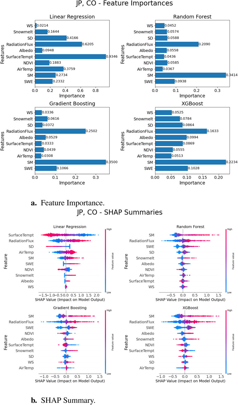
Figure 10. (A) Feature importance, and (B) SHAP summary results for Jones Pass, CO. Explanation of elements are mentioned in the caption of Figure 8.

In this study, we also conducted separate analyses for snow and no-snow seasons to better understand the impact of snow-related variables on CETB SSD variability. The snow season was defined as periods when both SWE and SD were greater than zero, indicating snow presence on the ground, while the no-snow season was defined as periods with zero SWE and SD, reflecting snow-free conditions. For each season, an RF model (the best-performing model) was trained and tested to evaluate the relationship between the predictor variables and the target variable, CETB SSDs (Table 5). By analyzing these two seasons separately, we aimed to isolate the influence of snow-related variables during periods of snow cover and compare them to periods without snow. This seasonal distinction provides deeper insights into the temporal dynamics of snow’s impact on microwave sensor measurements and allows us to assess whether snow-related factors are more significant drivers of SSD variability during snow-covered periods.

Table 5

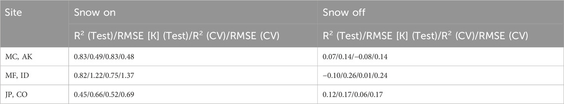
Table 5. Performance on test data and CV in snow and no-snow seasons.

The feature importance and SHAP analysis for MC, AK highlight key differences in the drivers of CETB SSD variability between snow and no-snow seasons (Figures 11A, 12A). During the snow season, RF performed well, with SWE emerging as the most significant predictor, driving higher SSD values. Other influential variables included SM, AirTemp, and SD, demonstrating the combined effects of snowpack dynamics and energy balance. High SM and warmer temperatures were associated with increased SSDs, while lower values corresponded to decreases. In contrast, the model struggled during the no-snow season, reflected in much lower R² values. During this period, NDVI, Albedo, SM, WS, SurfaceTempt, and RadiationFlux emerged as the dominant factors. Since SWE and SD were defined as zero during the no-snow season, their lack of influence reflects the absence of snow rather than a change in feature importance. Vegetation cover, reflected by higher NDVI, pushed SSD predictions upward, as expected, with surface and vegetation dynamics taking over in the absence of snow. Higher Albedo and SM also drove SSD predictions upward, but the model’s poor performance suggests that these factors alone do not fully capture SSD variability during the no-snow season. This seasonal shift underscores the changing dominance of snowpack processes during the snow season and surface and vegetation factors during the no-snow period.

Figure 11

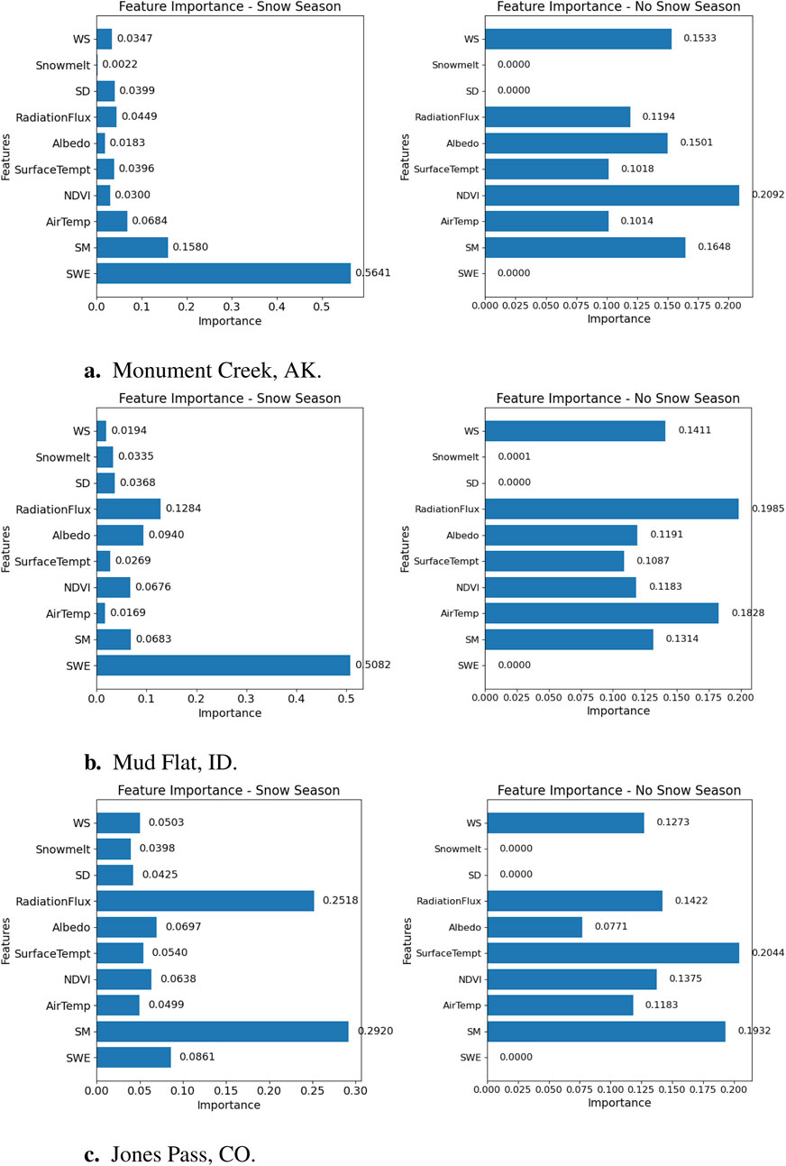
Figure 11. Feature importance results in snow and no-snow season across the three sites: (A) Monument Creek, AK, (B) Mud Flat, ID, and (C) Jones Pass, CO.

Figure 12

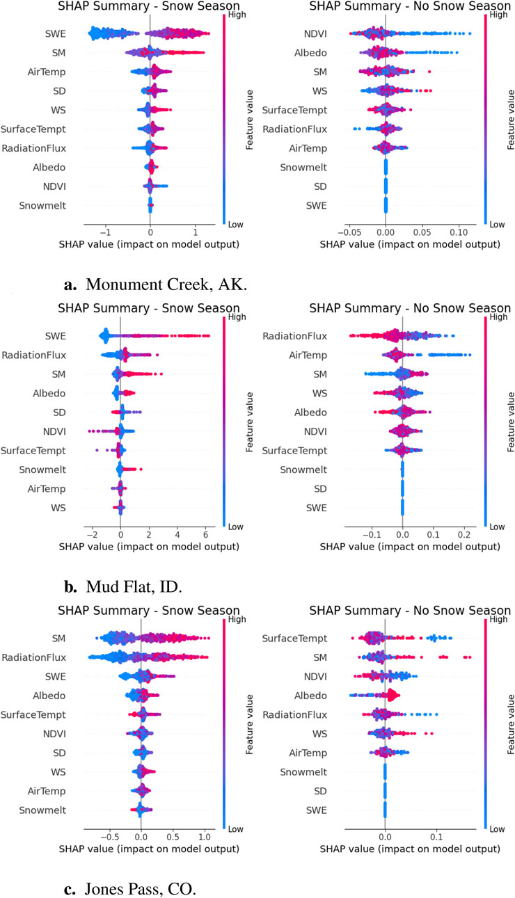
Figure 12. SHAP Summary results in snow and no-snow season across the three sites: (A) Monument Creek, AK, (B) Mud Flat, ID, and (C) Jones Pass, CO. Explanation of elements are mentioned in the caption of Figure 8.

At MF, the model revealed clear seasonal differences in CETB SSD drivers (Figures 11B, 12B). During the snow season, SWE was the most critical factor, consistently pushing SSD predictions higher. Other key variables included RadiationFlux, SM, Albedo, and SD, highlighting the influence of snowpack and energy fluxes. High values of SWE and SM push SSDs upward. In the no-snow season, RadiationFlux (having the greatest influence), AirTemp, and SM became the dominant variables. Despite the shift in dominant factors, the model’s poor performance in the no-snow season suggests these variables alone cannot explain SSD variability in the absence of snow. This seasonal transition emphasizes the higher relevance of surface energy and vegetation factors during the no-snow period.

For JP, the feature importance and SHAP analysis also revealed distinct seasonal shifts in SSD drivers (Figures 11C, 12C). In the snow season, SM was the most influential factor, with higher values driving SSD predictions upward. Other important contributors included RadiationFlux, SWE, and Albedo, showing the combined influence of subsurface moisture, snowpack, and energy balance. SurfaceTempt, NDVI, and SD played moderate roles, though less pronounced. In the no-snow season, SurfaceTempt, SM, and NDVI taking precedence. SM remained a key factor, though less dominant than during the snow season. The model’s lower performance during the no-snow season suggests that surface and energy factors alone cannot fully account for SSD variability when snow is absent, highlighting the shift from snowpack-driven processes to surface and energy dynamics.

4 Discussion

4.1 Key findings and implications

This study is the first to demonstrate the utility of site-specific CETB SSD variability for improving SWE estimations, addressing long-standing challenges in RS of snowpack in heterogeneous environments. The linear correlation results across all sites demonstrate that SSDs, particularly when smoothed, can be effective proxies for capturing a large part of the snowpack variability and could potentially enhance SWE estimations using PMW data in future studies. The correlations and time series analysis suggest that integrating SSDs into existing SWE retrieval algorithms, such as the Chang algorithm or ML techniques, can help mitigate discrepancies in SWE estimation, particularly during peak accumulation periods and when PMW signals become saturated.

The incorporation of site characteristics into snow depth retrieval models, as demonstrated by (Liu et al., 2024; Singh et al., 2024), underscores the importance of integrating auxiliary variables to account for spatial and environmental heterogeneity, particularly in complex terrains. Similarly, the potential of CETB SSDs in this study highlights their ability to capture the spatiotemporal variability of surface, snowpack, and atmospheric conditions, suggesting that leveraging SSDs alongside auxiliary factors could significantly improve the accuracy of SWE estimations in diverse and dynamic environments. Unlike traditional SWE retrieval methods that rely on static calculations and fixed empirical coefficients (e.g., the Chang algorithm), which fail to account for the spatial and temporal variability of snow characteristics and lead to errors in SD estimation (Yang et al., 2019), our dynamic, site-specific approach leverages CETB SSD to better capture snowpack variability, particularly in complex terrain such as JP in Colorado. This novel approach extends the applicability of SSDs to improve the accuracy and robustness of satellite-derived SWE estimates across diverse geographical regions. By addressing variability in snowpack characteristics, this approach advances snow monitoring capabilities, offering significant potential for hydrological modeling and environmental impact assessments.

4.2 Site-specific model performance

The feature importance analysis reveals notable differences in model performance across the three study sites. MC in AK consistently shows the highest model accuracy, with RF and XGBoost achieving test R² values of 0.89 and minimal RMSEs ranging from 0.37 to 0.39 (Table 4). In comparison, MF in ID exhibits moderate performance with R² values between 0.73 and 0.74 but higher RMSEs (0.97-0.98). JP in CO exhibits the weakest performance, with LR producing the lowest R² (0.44) and highest RMSE (0.71). However, XGBoost performs comparatively better at JP, achieving the best R² (0.63) and lower RMSE (0.58). These results emphasize that CETB SSD variability is most accurately predicted at MC, with moderate accuracy at MF and the least accuracy at JP, highlighting the challenges posed by site-specific factors and the need for tailored models that address local variability drivers at each site.

4.3 Performance under snow-on and snow-off conditions

A comparative analysis of snow-on and snow-off conditions reveals further insights into model performance and environmental drivers of SSD variability. (Table 5). At MC, models achieve high predictive accuracy during snow-on periods (R² = 0.83), but performance declines sharply during snow-off periods (R² = 0.07). Similarly, MF achieves strong snow-on performance (R² = 0.82) but struggles during snow-off conditions (R² = −0.10). In contrast, JP shows moderate snow-on performance (R² = 0.45) and comparatively better snow-off performance (R² = 0.12). These results indicate that the models perform more accurately during snow-on periods, driven by snowpack variables, but struggle to capture variability during snow-off periods. JP performs better in the no-snow season compared to other sites due to the persistent influence of SM, which remains a key driver year-round due to the site’s characteristics. This persistent variability in SM, along with energy balance factors such as RadiationFlux and SurfaceTempt, allows the model to effectively capture SSD variability even when snowpack variables are absent. In contrast, the models at MC in AK and MF in ID rely heavily on snowpack-related variables, which leads to poorer performance during the no-snow season. These findings underscore the importance of site-specific environmental drivers in determining SSD variability and highlight the need for tailored models that integrate additional non-snowpack variables in snow-off periods.

4.4 Environmental drivers of SSD variability

The feature importance and SHAP analyses reveal that environmental and snowpack conditions, as well as site-specific characteristics such as latitude and elevation, significantly shape CETB SSD variability. At MC, AK (65°N), SWE consistently emerges as the dominant factor across all models, especially in RF and XGBoost, reflecting the prolonged snow cover and substantial accumulation characteristic of high-latitude regions. SHAP values confirm the strong influence of SWE, with secondary contributions from SM, AirTemp, and RadiationFlux. Due to limited sunlight in winter, RadiationFlux becomes a more influential factor during spring and summer snowmelt. In contrast, vegetation (measured by NDVI) plays a minimal role at MC in Alaska, consistent with the region’s sparse vegetation.

At MF in ID (42°N), SWE remains the primary driver, particularly in tree-based models. However, factors such as RadiationFlux, SM, and NDVI also play significant roles. The semi-arid, mid-latitude environment of MF, ID, leads to a shorter snow season and increased solar radiation, making energy balance variables like RadiationFlux critical during snowmelt. SM also plays a key role in subsurface moisture dynamics, while denser vegetation compared to MC increases NDVI’s relevance. At JP, CO (39°N), SM emerges as the most influential factor across all models, driven by the short snow season and mountainous terrain. Although snow-related variables like SWE and SD contribute to SSD variability, SM, along with RadiationFlux and SurfaceTempt, has a greater impact. The complex terrain and dense vegetation at JP, CO, create spatial variability in SM-steep slopes facilitate rapid drainage, while valleys retain moisture. This variability significantly affects microwave emissions, making SM a critical driver of SSD variability. Additionally, the dense forest cover reduces snowpack exposure to sunlight and wind, stabilizing snow conditions and making SM a more critical factor in determining SSD variability. The relatively uniform snowpack at JP, CO, reduces the influence of SWE, shifting the focus toward subsurface moisture and energy balance factors. In contrast, the simpler terrain and sparse vegetation at MC and MF allow SWE to dominate SSD variability due to the microwave signal’s direct sensitivity to snowpack properties. The site comparisons highlight how latitude and elevation influence key drivers, with SWE dominating in high-latitude snow-heavy environments like MC in Alaska, and SM taking precedence in high-elevation, mid-latitude regions like JP in Colorado. At MF in Idaho, the interplay between SWE, RadiationFlux, and vegetation reflects the semi-arid, mid-latitude environment.

The comparisons across the three sites emphasize the influence of latitude, elevation, and terrain complexity in determining the primary drivers of SSD variability. At high-latitude sites such as MC, AK, SWE dominates due to prolonged snow cover and relatively simple terrain. In contrast, mid-latitude, high-elevation locations like JP, CO, rely more heavily on SM and energy balance variables, given the shorter snow season and complex terrain. Meanwhile, at MF, ID, the interplay between SWE, RadiationFlux, and vegetation reflects the semi-arid, mid-latitude environment, where both snowpack and energy balance factors contribute significantly to SSD variability. These findings highlight the need for site-specific adjustments in PMW-based SWE retrieval models to account for the varying environmental drivers across different regions. For example, in high-latitude regions like MC, AK, models should prioritize SWE, whereas in high-elevation sites like JP, CO, more weight should be given to SM and other energy balance variables. Additionally, these results also highlight the potential impact of biases in GLDAS SWE (a common negative bias in precipitation at higher altitudes and its impact on modeled SWE output). This could inflate correlations with other environmental variables, such as SurfaceTempt or SM, shifting the model’s interpretation of which features are most important in high-elevation, complex regions such as JP. Recognizing and addressing such biases is essential for accurately interpreting feature importance results, especially when analyzing the role of SWE and other snowpack variables across diverse landscapes.

4.5 Broader context and implications

Accurate SWE estimations derived from CETB SSD have significant potential to enhance hydrological models, supporting improved water resource management in snow-fed basins. By providing more reliable predictions of seasonal runoff, this approach is critical for flood mitigation and drought preparedness. Beyond snow research, the insights gained from CETB SSD can inform models of other environmental variables in snow-dominated regions, including vegetation dynamics, soil moisture variability, permafrost conditions, and snowmelt processes. These applications could contribute to more accurate environmental predictions and strengthen the effectiveness of water resource management strategies, particularly in regions where snowpack plays a vital role in the hydrological cycle.

4.6 Limitations and future directions

While this study highlights the transformative potential of CETB SSDs for improving SWE estimations, several limitations must be acknowledged. First, the reliance on GLDAS data introduces biases, particularly in high-altitude regions, which may affect model performance and the interpretation of feature importance. Addressing these biases is crucial to enhance the robustness of future analyses. Second, the study’s focus on three sites limits the generalizability of the findings. Expanding the analysis to include diverse terrains and climatic conditions, such as polar or tropical montane regions, could broaden the applicability of the approach. Third, the models demonstrate strong performance during snow-on periods but experience reduced accuracy during snow-off conditions. This highlights the need to better integrate non-snowpack variables such as soil moisture, vegetation, and energy fluxes.

Future research will explore ways to incorporate CETB SSDs directly into SWE retrieval algorithms under both wet and dry snow conditions, as microwave signals interact differently based on liquid water content (Kang et al., 2013). An interesting approach could involve leveraging adaptive computational models to account for site-specific variability in pixels or regions. These integrations could enhance the precision of PMW-based SWE estimation methods. Future research should incorporate a sensitivity analysis to refine feature selection for SWE estimation, ensuring that only the most relevant variables are included. While this study focuses on analyzing CETB SSD variability rather than directly predicting SWE, our next study will apply weighted ranking methods and feature selection techniques to improve ML model performance by prioritizing key predictors such as CETB SSDs, NDSI, fractional snow cover, and PMW channels. Incorporating high-resolution ancillary datasets will further improve model adaptability and performance across seasons. Testing this methodology in glacial or tropical snowpack regions could validate its applicability in diverse climatic settings. Additionally, leveraging advanced ML techniques and ensemble approaches could enhance predictive accuracy and mitigate model biases. Exploring the integration of physical snow models, such as the Snow Microwave Radiative Transfer (SMRT) model, would provide deeper insights into the relationship between CETB SSDs and snowpack dynamics, further refining SWE estimation techniques. The retrieval of SD and SWE using PMW RS faces significant uncertainties due to factors such as signal saturation in deep snowpacks, the presence of liquid water within the snowpack, and the spatial and temporal variability of snow properties, particularly grain size (Dai et al., 2023). Extending the analysis to other RS datasets and frequencies could enhance the robustness of CETB SSD applications. For instance, testing additional frequencies might better account for varying snow conditions, such as deep or shallow snowpacks. Dynamic models that adapt to seasonal shifts in snowpack and environmental drivers could further improve predictive accuracy for both snow-covered and snow-free landscapes. These efforts will support the development of more accurate SWE estimations, which is critical for water resource management, hazard mitigation, and environmental modeling.

5 Conclusion

This study provides a detailed analysis of CETB SSD variability and its environmental drivers across three geographically and climatically distinct sites: Monument Creek, AK; Mud Flat, ID; and Jones Pass, CO. Using machine learning-based feature importance analysis, SWE consistently emerged as the dominant driver at high-latitude sites like MC and MF, while soil moisture played a more critical role at JP due to its high elevation and complex terrain. Seasonal comparisons revealed distinct shifts in SSD drivers, with SWE, RadiationFlux, and SM dominating during snow-on periods, while SurfaceTempt, SM, and vegetation variables like NDVI gained prominence during snow-off periods. These shifts emphasize the versatility of CETB SSDs in capturing seasonal changes in snowpack, soil moisture, and vegetation. The findings demonstrate the potential of CETB SSDs to improve SWE estimations and provide valuable insights into other environmental variables such as SM, energy fluxes, and vegetation cover. By monitoring SSD changes in relation to observed, ground-based seasonal SWE variations, we can enhance the potential for more accurate SWE estimation across different stages of the snow season. Leveraging the potential of SSD not only improves RS methodologies but also deepens the interpretive accuracy of satellite-derived cryospheric datasets, leading to a more nuanced understanding and modeling of snowpack dynamics and their hydrological implications. By addressing site-specific variability and adapting to diverse snowpack and environmental conditions, this approach advances RS capabilities for hydrological and environmental modeling. Future efforts to expand this research into different regions, integrate dynamic models, and refine physical snow models will further enhance the applicability of CETB SSD-based techniques. As snowpack dynamics worldwide continues changing, these advancements will play a crucial role in managing water resources, ecosystems, and agriculture in snow-affected regions, as well as mitigating natural hazards and improving environmental predictions. This study offers a robust framework for improving SWE estimations and contributes to advancing RS techniques for monitoring snow-affected regions under changing environmental conditions.

Data availability statement

The original contributions presented in the study are included in the article/Supplementary Material, further inquiries can be directed to the corresponding author.

Author contributions

MBo: Conceptualization, Formal analysis, Investigation, Methodology, Software, Validation, Visualization, Writing–original draft, Writing–review and editing. JR: Conceptualization, Investigation, Project administration, Software, Resources, Supervision, Validation, Writing–review and editing. MBr: Conceptualization, Investigation, Software, Resources, Validation, Writing–review and editing. DL: Conceptualization, Investigation, Resources, Validation, Writing–review and editing. MH: Conceptualization, Investigation, Software, Resources, Validation, Writing–review and editing. H-PM: Conceptualization, Validation, Writing–review and editing.

Funding

The author(s) declare that financial support was received for the research, authorship, and/or publication of this article. This work was not supported by external funding. Partial funding from the Lehigh University College of Arts and Sciences Research Fellowship supported this project.

Acknowledgments

We sincerely thank Shad O’Neel, Frank Pazzaglia, and Barton Forman for their valuable insights and expertise. We also extend our gratitude to the data sources (SNOTEL, NSIDC, and NASA) that played a crucial role in enabling the findings of this study. Lastly, we acknowledge the Lehigh University College of Arts and Sciences Research Fellowship for supporting MBo in initiating this work.

Conflict of interest

The authors declare that the research was conducted in the absence of any commercial or financial relationships that could be construed as a potential conflict of interest.

Generative AI statement

The author(s) declare that no Generative AI was used in the creation of this manuscript.

Publisher’s note

All claims expressed in this article are solely those of the authors and do not necessarily represent those of their affiliated organizations, or those of the publisher, the editors and the reviewers. Any product that may be evaluated in this article, or claim that may be made by its manufacturer, is not guaranteed or endorsed by the publisher.

Supplementary material

The Supplementary Material for this article can be found online at: https://www.frontiersin.org/articles/10.3389/frsen.2025.1554084/full#supplementary-material

Footnotes

¹The elevation range is calculated within an approximate area of 5.5 km surrounding the site.

²ArcticDEM with 2 m resolution (Porter et al., 2018).

³Shuttle Radar Topography Mission (SRTM) Digital Elevation Model with 30 m resolution (Farr et al., 2007).

References

Adam, J. C., Hamlet, A. F., and Lettenmaier, D. P. (2009). Implications of global climate change for snowmelt hydrology in the twenty-first century. Hydrological Process. Int. J. 23, 962–972. doi:10.1002/hyp.7201

CrossRef Full Text | Google Scholar

Armstrong, R. L., and Brodzik, M. J. (2001). Recent Northern Hemisphere snow extent: a comparison of data derived from visible and microwave satellite sensors. Geophys. Res. Lett. 28, 3673–3676. doi:10.1029/2000GL012556

CrossRef Full Text | Google Scholar

Armstrong, R. L., and Brodzik, M. J. (2002). Hemispheric-scale comparison and evaluation of passive-microwave snow algorithms. Ann. Glaciol. 34, 38–44. doi:10.3189/172756402781817428

CrossRef Full Text | Google Scholar

Aydin, H. E., and Iban, M. C. (2023). Predicting and analyzing flood susceptibility using boosting-based ensemble machine learning algorithms with SHapley Additive exPlanations. Nat. Hazards 116, 2957–2991. doi:10.1007/s11069-022-05793-y

CrossRef Full Text | Google Scholar

Barnett, T. P., Adam, J. C., and Lettenmaier, D. P. (2005). Potential impacts of a warming climate on water availability in snow-dominated regions. Nature 438, 303–309. doi:10.1038/nature04141

PubMed Abstract | CrossRef Full Text | Google Scholar

Beaudoing, H., and Rodell, M. (2020). GLDAS Noah land surface model L4 3 hourly 0.25 x 0.25 degree V2.1. doi:10.5067/E7TYRXPJKWOQ

CrossRef Full Text | Google Scholar

Breiman, L. (2001). Random forests. Mach. Learn. 45, 5–32. doi:10.1023/A:1010933404324

CrossRef Full Text | Google Scholar

Brodzik, M., and Long, D. (2018). Calibrated passive microwave daily EASE-Grid 2.0 brightness temperature ESDR (CETB): algorithm theoretical basis Document. MEaSUREs Project White Paper: Boulder, CO, USA. doi:10.5281/zenodo.7958456

CrossRef Full Text | Google Scholar

Brodzik, M., Long, D., Hardman, M., Paget, A., and Armstrong, R. (2016). MEaSUREs calibrated enhanced-resolution passive microwave daily EASE-grid 2.0 brightness temperature ESDR, version 1. NASA National Snow and Ice Data Center Distributed Active Archive Center: Boulder, CO, USA. doi:10.5067/MEASURES/CRYOSPHERE/NSIDC-0630.001

CrossRef Full Text | Google Scholar

Chang, A., Foster, J., Hall, D., Goodison, B. E., Walker, A. E., Metcalfe, J., et al. (1997). Snow parameters derived from microwave measurements during the BOREAS winter field campaign. J. Geophys. Res. Atmos. 102, 29663–29671. doi:10.1029/96JD03327

CrossRef Full Text | Google Scholar

Chang, A. T., Foster, J. L., and Hall, D. K. (1987). Nimbus-7 SMMR derived global snow cover parameters. Ann. Glaciol. 9, 39–44. doi:10.3189/S0260305500200736

CrossRef Full Text | Google Scholar

Chang, A. T., Foster, J. L., Hall, D. K., Rango, A., and Hartline, B. K. (1982). Snow water equivalent estimation by microwave radiometry. Cold Regions Sci. Technol. 5, 259–267. doi:10.1016/0165-232X(82)90019-2

CrossRef Full Text | Google Scholar

Chang, T., Gloersen, P., Schmugge, T., Wilheit, T., and Zwally, H. (1976). Microwave emission from snow and glacier ice. J. Glaciol. 16, 23–39. doi:10.3189/S0022143000031415

CrossRef Full Text | Google Scholar

Chen, T., and Guestrin, C. (2016). “Xgboost: a scalable tree boosting system,” in Proceedings of the 22nd acm sigkdd international conference on knowledge discovery and data mining, 785–794. doi:10.1145/2939672.2939785

CrossRef Full Text | Google Scholar

Cho, E., Vuyovich, C. M., Kumar, S. V., Wrzesien, M. L., and Kim, R. S. (2023). Evaluating the utility of active microwave observations as a snow mission concept using observing system simulation experiments. Cryosphere 17, 3915–3931. doi:10.5194/tc-17-3915-2023

CrossRef Full Text | Google Scholar

Cook, B. I., Mankin, J. S., and Anchukaitis, K. J. (2018). Climate change and drought: from past to future. Curr. Clim. Change Rep. 4, 164–179. doi:10.1007/s40641-018-0093-2

CrossRef Full Text | Google Scholar

Dai, L.-Y., Ma, L.-J., Nie, S.-P., Wei, S.-Y., and Che, T. (2023). Historical and real-time estimation of snow depth in Eurasia based on multiple passive microwave data. Adv. Clim. Change Res. 14, 537–545. doi:10.1016/j.accre.2023.07.003

CrossRef Full Text | Google Scholar

Canada, N. R. (2015). Microwave remote sensing. Available at: https://natural-resources.canada.ca/maps-tools-and-publications/satellite-imagery-elevation-data-and-air-photos/tutorial-fundamentals-remote-sensing/microwave-remote-sensing/9371 (Accessed October, 2024).

Google Scholar

Didan, K. (2015). MOD13A1 MODIS/Terra vegetation indices 16-day L3 global 500m SIN grid V006. doi:10.5067/MODIS/MOD13A1.006

CrossRef Full Text | Google Scholar

SNOTEL (2024). SNOwpack TELemetry network (SNOTEL). United States, US department of agriculture, natural resource conservation Service, national water and climate center, Air and water database. Water Clim. Inf. Syst.

Google Scholar

Dewitz, J. (2023). National land cover database (NLCD) 2021 products. U.S. Geol. Surv. data release. doi:10.5066/P9JZ7AO3

CrossRef Full Text | Google Scholar

Farr, T. G., Rosen, P. A., Caro, E., Crippen, R., Duren, R., Hensley, S., et al. (2007). The shuttle radar topography mission. Rev. Geophys. 45. doi:10.1029/2005RG000183

CrossRef Full Text | Google Scholar

Fazli, S., Fisher, J. B., Li, W., Thomas, R., Grisel Todorov, N., Perera, S., et al. (2023). Cultivating climate resilience: hydrological shifts and agricultural strategies in California’s central valley. AGU Fall Meet. Abstr. 2023, H33I–H1906.

Google Scholar

Foster, J., Chang, A., and Hall, D. (1997). Comparison of snow mass estimates from a prototype passive microwave snow algorithm, a revised algorithm and a snow depth climatology. Remote Sens. Environ. 62, 132–142. doi:10.1016/S0034-4257(97)00085-0

CrossRef Full Text | Google Scholar

Foster, J. L., Sun, C., Walker, J. P., Kelly, R., Chang, A., Dong, J., et al. (2005). Quantifying the uncertainty in passive microwave snow water equivalent observations. Remote Sens. Environ. 94, 187–203. doi:10.1016/j.rse.2004.09.012

CrossRef Full Text | Google Scholar

Friedman, J. H. (2001). Greedy function approximation: a gradient boosting machine. Ann. statistics 29, 1189–1232. doi:10.1214/aos/1013203451

CrossRef Full Text | Google Scholar

Han, S., Liu, B., Shi, C., Liu, Y., Qiu, M., and Sun, S. (2020). Evaluation of CLDAS and GLDAS datasets for Near-surface Air Temperature over major land areas of China. Sustainability 12, 4311. doi:10.3390/su12104311

CrossRef Full Text | Google Scholar

Hoogendoorn, G., Stockigt, L., Saarinen, J., and Fitchett, J. M. (2021). Adapting to climate change: the case of snow-based tourism in Afriski, Lesotho. Afr. Geogr. Rev. 40, 92–104. doi:10.1080/19376812.2020.1773878

CrossRef Full Text | Google Scholar

Huning, L. S., and AghaKouchak, A. (2020). Global snow drought hot spots and characteristics. Proc. Natl. Acad. Sci. 117, 19753–19759. doi:10.1073/pnas.1915921117

PubMed Abstract | CrossRef Full Text | Google Scholar

Jiang, L., Shi, J., Tjuatja, S., Chen, K. S., Du, J., and Zhang, L. (2010). Estimation of snow water equivalence using the polarimetric scanning radiometer from the cold land processes experiments (CLPX03). IEEE Geoscience Remote Sens. Lett. 8, 359–363. doi:10.1109/LGRS.2010.2076345

CrossRef Full Text | Google Scholar

Johnson, M. T., Ramage, J., Troy, T. J., and Brodzik, M. J. (2020). Snowmelt detection with calibrated, enhanced-resolution brightness temperatures (CETB) in Colorado watersheds. Water Resour. Res. 56. doi:10.1029/2018WR024542

CrossRef Full Text | Google Scholar

Kang, D. H., Barros, A. P., and Dery, S. J. (2013). Evaluating passive microwave radiometry for the dynamical transition from dry to wet snowpacks. IEEE Trans. Geoscience Remote Sens. 52, 3–15. doi:10.1109/TGRS.2012.2234468

CrossRef Full Text | Google Scholar

Kelly, R. E., Chang, A. T., Tsang, L., and Foster, J. L. (2003). A prototype AMSR-E global snow area and snow depth algorithm. IEEE Trans. Geoscience Remote Sens. 41, 230–242. doi:10.1109/TGRS.2003.809118

CrossRef Full Text | Google Scholar

Kim, Y., and Van Zyl, J. J. (2009). A time-series approach to estimate soil moisture using polarimetric radar data. IEEE Trans. Geoscience Remote Sens. 47, 2519–2527. doi:10.1109/TGRS.2009.2014944

CrossRef Full Text | Google Scholar

Li, D., Lettenmaier, D. P., Margulis, S. A., and Andreadis, K. (2019). The role of rain-on-snow in flooding over the conterminous United States. Water Resour. Res. 55, 8492–8513. doi:10.1029/2019WR024950

CrossRef Full Text | Google Scholar

Li, D., Wrzesien, M. L., Durand, M., Adam, J., and Lettenmaier, D. P. (2017). How much runoff originates as snow in the western United States, and how will that change in the future? Geophys. Res. Lett. 44, 6163–6172. doi:10.1002/2017GL073551

CrossRef Full Text | Google Scholar

Li, Z. (2022). Extracting spatial effects from machine learning model using local interpretation method: an example of SHAP and XGBoost. Comput. Environ. Urban Syst. 96, 101845. doi:10.1016/j.compenvurbsys.2022.101845

CrossRef Full Text | Google Scholar

Liang, S., and Wang, J. (2020). “Chapter 19 - snow water equivalent,” in Advanced remote sensing. Second EditionSecond edition edn. (Academic Press), 713–763. doi:10.1016/B978-0-12-815826-5.00019-2

CrossRef Full Text | Google Scholar

Liston, G., and Sturm, M. (2021). Global seasonal-snow classification. doi:10.5067/99FTCYYYLAQ0

CrossRef Full Text | Google Scholar

Liu, Q., Gui, D., Zhang, L., Niu, J., Dai, H., Wei, G., et al. (2022). Simulation of regional groundwater levels in arid regions using interpretable machine learning models. Sci. Total Environ. 831, 154902. doi:10.1016/j.scitotenv.2022.154902

PubMed Abstract | CrossRef Full Text | Google Scholar

Liu, Y., Yang, J., Chen, X., Yao, J., Li, L., and Qiu, Y. (2024). Moderate-resolution snow depth product retrieval from passive microwave brightness data over Xinjiang using machine learning approach. Int. J. Digital Earth 17, 2299208. doi:10.1080/17538947.2023.2299208

CrossRef Full Text | Google Scholar

Long, D. G., and Brodzik, M. J. (2015). Optimum image formation for spaceborne microwave radiometer products. IEEE Trans. Geoscience remote Sens. 54, 2763–2779. doi:10.1109/TGRS.2015.2505677

PubMed Abstract | CrossRef Full Text | Google Scholar

Lu, H., Chen, M., and Kuang, W. (2020). The impacts of abnormal weather and natural disasters on transport and strategies for enhancing ability for disaster prevention and mitigation. Transp. Policy 98, 2–9. doi:10.1016/j.tranpol.2019.10.006

CrossRef Full Text | Google Scholar

Lundberg, S. (2017). A unified approach to interpreting model predictions. arXiv Prepr. arXiv:1705.07874. doi:10.48550/arXiv.1705.07874

CrossRef Full Text | Google Scholar

Markus, T., Powell, D. C., and Wang, J. R. (2005). Sensitivity of passive microwave snow depth retrievals to weather effects and snow evolution. IEEE Trans. Geoscience Remote Sens. 44, 68–77. doi:10.1109/TGRS.2005.860208

CrossRef Full Text | Google Scholar

Mätzler, C. (1994). Passive microwave signatures of landscapes in winter. Meteorology Atmos. Phys. 54, 241–260. doi:10.1007/BF01030063

CrossRef Full Text | Google Scholar

Montgomery, D. C., Peck, E. A., and Vining, G. G. (2021). Introduction to linear regression analysis. John Wiley & Sons.

Google Scholar

Njoku, E. G., and Kong, J.-A. (1977). Theory for passive microwave remote sensing of near-surface soil moisture. J. Geophys. Res. 82, 3108–3118. doi:10.1029/JB082i020p03108

CrossRef Full Text | Google Scholar

Ntokas, K. F., Odry, J., Boucher, M.-A., and Garnaud, C. (2021). Investigating ANN architectures and training to estimate snow water equivalent from snow depth. Hydrology Earth Syst. Sci. 25, 3017–3040. doi:10.5194/hess-25-3017-2021

CrossRef Full Text | Google Scholar

Omatsu, K., Uchiyama, M., Shimizu, U., Ling, Y., Okuda, S., and Koyama, Y. (2023). Impact of heavy snowfall on emergency transport and prognosis of out-of-hospital cardiac arrest patients: a nation-wide cohort study. Prehospital Disaster Med. 38, 436–443. doi:10.1017/s1049023x23006040

PubMed Abstract | CrossRef Full Text | Google Scholar

Picard, G., Leduc-Leballeur, M., Banwell, A. F., Brucker, L., and Macelloni, G. (2022). The sensitivity of satellite microwave observations to liquid water in the Antarctic snowpack. Cryosphere 16, 5061–5083. doi:10.5194/tc-16-5061-2022

CrossRef Full Text | Google Scholar

Porter, C., Morin, P., Howat, I., Noh, M.-J., Bates, B., Peterman, K., et al. (2018). ArcticDEM. doi:10.7910/DVN/OHHUKH

CrossRef Full Text | Google Scholar

Pulliainen, J., and Hallikainen, M. (2001). Retrieval of regional snow water equivalent from space-borne passive microwave observations. Remote Sens. Environ. 75, 76–85. doi:10.1016/S0034-4257(00)00157-7

CrossRef Full Text | Google Scholar

Qin, Y., Abatzoglou, J. T., Siebert, S., Huning, L. S., AghaKouchak, A., Mankin, J. S., et al. (2020). Agricultural risks from changing snowmelt. Nat. Clim. Change 10, 459–465. doi:10.1038/s41558-020-0746-8

CrossRef Full Text | Google Scholar

Rixen, C., Høye, T. T., Macek, P., Aerts, R., Alatalo, J. M., Anderson, J. T., et al. (2022). Winters are changing: snow effects on Arctic and alpine tundra ecosystems. Arct. Sci. 8, 572–608. doi:10.1139/as-2020-0058

CrossRef Full Text | Google Scholar

Rodell, M., Houser, P., Jambor, U., Gottschalck, J., Mitchell, K., Meng, C.-J., et al. (2004). The global land data assimilation system. Bull. Am. Meteorological Soc. 85, 381–394. doi:10.1175/BAMS-85-3-381

CrossRef Full Text | Google Scholar

Saberi, N., Kelly, R., Flemming, M., and Li, Q. (2020). Review of snow water equivalent retrieval methods using spaceborne passive microwave radiometry. Int. J. Remote Sens. 41, 996–1018. doi:10.1080/01431161.2019.1654144

CrossRef Full Text | Google Scholar

Salas, H. D., Valencia, J., Builes-Jaramillo, A., and Jaramillo, A. (2022). Synoptic time scale variability in precipitation and streamflows for river basins over northern South America. Hydrology 9, 59. doi:10.3390/hydrology9040059

CrossRef Full Text | Google Scholar

Sapiano, M. R., Berg, W. K., McKague, D. S., and Kummerow, C. D. (2012). Toward an intercalibrated fundamental climate data record of the SSM/I sensors. IEEE Trans. Geoscience Remote Sens. 51, 1492–1503. doi:10.1109/TGRS.2012.2206601

CrossRef Full Text | Google Scholar

Singh, D. K., Tanniru, S., Singh, K. K., Negi, H. S., and Ramsankaran, R. (2024). Passive microwave remote-sensing-based high-resolution snow depth mapping for Western Himalayan zones using multifactor modeling approach. Cryosphere 18, 451–474. doi:10.5194/tc-18-451-2024

CrossRef Full Text | Google Scholar

Slatyer, R. A., Umbers, K. D., and Arnold, P. A. (2022). Ecological responses to variation in seasonal snow cover. Conserv. Biol. 36, e13727. doi:10.1111/cobi.13727

PubMed Abstract | CrossRef Full Text | Google Scholar

Tait, A. (1998). Estimation of snow water equivalent using passive microwave radiation data. Remote Sens. Environ. 64, 286–291. doi:10.1016/S0034-4257(98)00005-4

CrossRef Full Text | Google Scholar

Takala, M., Luojus, K., Pulliainen, J., Derksen, C., Lemmetyinen, J., Kärnä, J.-P., et al. (2011). Estimating northern hemisphere snow water equivalent for climate research through assimilation of space-borne radiometer data and ground-based measurements. Remote Sens. Environ. 115, 3517–3529. doi:10.1016/j.rse.2011.08.014

CrossRef Full Text | Google Scholar

Tanniru, S., and Ramasankaran, R. (2023). Machine learning based estimation of high-resolution snow depth in Alaska using passive microwave remote sensing data. IEEE J. Sel. Top. Appl. Earth Observations Remote Sens. 16, 6007–6025. doi:10.1109/JSTARS.2023.3287410

CrossRef Full Text | Google Scholar

Tanniru, S., and Ramsankaran, R. (2023). Passive microwave remote sensing of snow depth: techniques, challenges and future directions. Remote Sens. 15, 1052. doi:10.3390/rs15041052

CrossRef Full Text | Google Scholar

Temimi, M., Lakhankar, T., Zhan, X., Cosh, M. H., Krakauer, N., Fares, A., et al. (2014). Soil moisture retrieval using ground-based L-band passive microwave observations in northeastern USA. Vadose Zone J. 13, 1–10. doi:10.2136/vzj2013.06.0101

CrossRef Full Text | Google Scholar

Thackeray, C. W., Derksen, C., Fletcher, C. G., and Hall, A. (2019). Snow and climate: feedbacks, drivers, and indices of change. Curr. Clim. Change Rep. 5, 322–333. doi:10.1007/s40641-019-00143-w

CrossRef Full Text | Google Scholar

Tsang, L., Kong, J., and Shin, R. (1985). Theory of microwave. Remote Sens.

Google Scholar

Vander Jagt, B. J., Durand, M. T., Margulis, S. A., Kim, E. J., and Molotch, N. P. (2013). The effect of spatial variability on the sensitivity of passive microwave measurements to snow water equivalent. Remote Sens. Environ. 136, 163–179. doi:10.1016/j.rse.2013.05.002

CrossRef Full Text | Google Scholar

Wei, Y., Li, X., Gu, L., Zheng, X., and Jiang, T. (2023). A novel fine-resolution snow depth retrieval model to reveal detailed spatiotemporal patterns of snow cover in Northeast China. Int. J. Digital Earth 16, 1164–1185. doi:10.1080/17538947.2023.2196446

CrossRef Full Text | Google Scholar

Wei, Y., Li, X., Gu, L., Zheng, X., Jiang, T., and Zheng, Z. (2022). A fine-resolution snow depth retrieval algorithm from enhanced-resolution passive microwave brightness temperature using machine learning in Northeast China. IEEE Geoscience Remote Sens. Lett. 19, 1–5. doi:10.1109/LGRS.2022.3196135

CrossRef Full Text | Google Scholar

Westerling, A. L. (2016). Increasing western US forest wildfire activity: sensitivity to changes in the timing of spring. Philosophical Trans. R. Soc. B Biol. Sci. 371. doi:10.1098/rstb.2015.0178

PubMed Abstract | CrossRef Full Text | Google Scholar

Wiesmann, A., and Mätzler, C. (1999). Microwave emission model of layered snowpacks. Remote Sens. Environ. 70, 307–316. doi:10.1016/S0034-4257(99)00046-2

CrossRef Full Text | Google Scholar

Xiao, X., Zhang, T., Zhong, X., Shao, W., and Li, X. (2018). Support vector regression snow-depth retrieval algorithm using passive microwave remote sensing data. Remote Sens. Environ. 210, 48–64. doi:10.1016/j.rse.2018.03.008

CrossRef Full Text | Google Scholar

Xiong, C., Yang, J., Pan, J., Lei, Y., and Shi, J. (2022). Mountain snow depth retrieval from optical and passive microwave remote sensing using machine learning. IEEE Geoscience Remote Sens. Lett. 19, 1–5. doi:10.1109/LGRS.2022.3226204

CrossRef Full Text | Google Scholar

Yang, J., Jiang, L., Luojus, K., Pan, J., Lemmetyinen, J., Takala, M., et al. (2020). Snow depth estimation and historical data reconstruction over China based on a random forest machine learning approach. Cryosphere 14, 1763–1778. doi:10.5194/tc-14-1763-2020

CrossRef Full Text | Google Scholar

Yang, J., Jiang, L., Pan, J., Shi, J., Wu, S., Wang, J., et al. (2022). Comparison of machine learning-based snow depth estimates and development of a new operational retrieval algorithm over China. Remote Sens. 14, 2800. doi:10.3390/rs14122800

CrossRef Full Text | Google Scholar

Yang, J., Jiang, L., Wu, S., Wang, G., Wang, J., and Liu, X. (2019). Development of a snow depth estimation algorithm over China for the FY-3D/MWRI. Remote Sens. 11, 977. doi:10.3390/rs11080977

CrossRef Full Text | Google Scholar

Glossary

AMSR-E Advanced Microwave Spectroradiometer for EOS

AirTemp Air Temperature

ANNs Artificial Neural Networks

(T_b) Brightness Temperatures

CETB Calibrated Enhanced-Resolution Brightness Temperatures

CV Cross-Validation

DMRT Dense Media Radiative Transfer

RadiationFlux Downward Short-wave Radiation Flux

XGBoost Extreme Gradient Boosting

GLDAS Global Land Data Assimilation System

GES DISC Goddard Earth Sciences Data and Information Services Center

GEE Google Earth Engine

GBoost Gradient Boosting

SDGRD GRD standard deviation

GridSearchCV Grid Search Cross-Validation

H-pol Horizontal Polarization

IQR Interquartile Range

JP Jones Pass

K Kelvin

LR Linear Regression

ML Machine Learning

RMSE Root Mean Squared Error

MEMLS Microwave Emission Model for Layered Snowpacks

MODIS Moderate Resolution Imaging Spectroradiometer

MC Monument Creek

MF Mud Flat

NASA National Aeronautics and Space Administration

NSIDC National Snow and Ice Data Center

NRCS Natural Resources Conservation Service

NDVI Normalized Difference Vegetation Index

PMW Passive Microwave

RF Random Forest

RS Remote Sensing

rSIR Scatterometer Image Reconstruction

SMMR Scanning Multi-channel Microwave Radiometer

SHAP SHapley Additive exPlanations

SD Snow Depth

SWE Snow Water Equivalent

SNOTEL SNOpack TELemetry

SM Soil Moisture

SSD Spatial Standard Deviation

SSM/I Special Sensor Microwave Imager

SSMIS Special Sensor Microwave Imager/Sounder

SVM Support Vector Machine

SurfaceTempt Surface Temperature

USDA United States Department of Agriculture

V-pol Vertical Polarization

WS Wind Speed