Sentinel-1 (S1) time series alignment method for rapeseed fields mapping

Introduction: This paper presents a comprehensive analysis of rapeseed fields mapping using Sentinel-1 (S1) time series data. We applied a time series alignment method to enhance the accuracy of rapeseed fields detection, even in scenarios where reference label data are limited or not available.

Methods: To this end, for five different study sites in France and North America, we first investigated the temporal transferability of the classifiers across several years within the same site, specifically using the Random Forest (RF) and InceptionTime algorithms. We then examined the spatiotemporal transferability of the classifiers when a classifier trained on one site and year was used to generate rapeseed fields map for another site and year. Next, we proposed an S1 time series alignment method to improve classification accuracy across sites and years by accounting for temporal shifts caused by differences in agricultural practices and climatic conditions between sites.

Results and discussion: The main results demonstrated that rapeseed detection for 1 year, using training data from another year within the same site, achieved high accuracy, with F1 scores ranging from 85.5% to 97% for RF and from 88.2% to 98.3% for InceptionTime. When classifying using one-year training data from one site to classify another year in a different site, F1 scores varied between 48.8% and 97.7% for both RF and InceptionTime. Using a three year training dataset from one site to classify rapeseed fields in another site resulted in F1 scores ranging from 82.7% to 97.8% with RF and from 88.7% to 97.1% with InceptionTime. The proposed alignment method, designed to enhance classification using training and test data from different sites, improved F1 scores by up to 46.7%. These findings confirm the feasibility of mapping rapeseed with S1 images across various sites and years, highlighting its potential for both national and international agricultural monitoring initiatives.

1 Introduction

Mapping rapeseed fields plays a crucial role in agricultural management as rapeseed being a major source for oilseed, protein meal, livestock feed, and industrial liquid biofuels (Baka and Roland-Holst, 2009; Duren et al., 2015). Accurately monitoring the distribution and characteristics of rapeseed fields enables farmers and decision-makers to make informed decisions regarding fertilizer application, optimize harvest dates, and estimate yield (Zhang et al., 2022).

The extensive volume of available earth observation data, combined with machine learning (ML) techniques, has demonstrated a significant ability to provide accurate monitoring of croplands (Mercier et al., 2020; Huang et al., 2022; Shorachi et al., 2022; Sun et al., 2024). In particular, the integration of remote sensing and machine learning algorithms offers significant advantages for rapeseed monitoring through both after-season and mid-season classification (Maleki et al., 2024). Most satellite-based rapeseed fields mapping methods using optical imagery rely on the unique optical spectral signature of rapeseed (Wang et al., 2018; Han et al., 2021a). Specifically, the distinctive yellow color of rapeseed during its flowering stage has been utilized in various studies for identifying rapeseed fields (Wang et al., 2018; d’Andrimont et al., 2020; Han et al., 2021a; Chen et al., 2022). Based on this spectral feature, the Ratio Oilseed Rape Colorimetric Index (RRCI) and the Normalized Rapeseed Flowering Index (NRFI) were developed by Wang et al. (2018) and Han et al. (2021a), respectively. Meanwhile, methods using Synthetic Aperture Radar (SAR) images rely on the period of high SAR backscatter during stem elongation, inflorescence emergence, and fruit development of rapeseed (Veloso et al., 2017; Ashourloo et al., 2019; Maleki et al., 2023; 2024). Using these spectral and SAR features, many studies have reported high accuracy in rapeseed detection using training and test data from the same site (Pan et al., 2013; Sulik and Long, 2015; Zhang et al., 2022; Maleki et al., 2023).

There are several challenges in rapeseed classification. One challenge lies in the application of spectral index thresholds to detect rapeseed. While thresholds from specific study sites can be helpful, they may not apply well to other areas (Han et al., 2021b). Additionally, many rapeseed classification studies produce rapeseed maps based on peak flowering dates (Ashourloo et al., 2019; Chen et al., 2022), which vary by area due to differences in environmental conditions and cultivation practices, especially over large regions (Sulik and Long, 2015; Han et al., 2021a; Sun et al., 2024). Furthermore, the rapeseed growth cycle can differ in duration, with variable start and end times across different years and sites (Maleki et al., 2023). Consequently, achieving accurate rapeseed field mapping at fine resolutions over expansive areas remains a substantial challenge. In addition, misclassification between rapeseed and other crops reduces classification accuracy. Our previous study on rapeseed detection showed that the main misclassification occurs between rapeseed, peas, and fallow lands (Maleki et al., 2024). Another challenge of rapeseed mapping lies in its reliance on training samples obtained through time-consuming and expensive field campaigns, as well as the necessity for real ground data from various years and regions (Zhang et al., 2022). Traditional techniques often struggle to generalize to new data from different growing seasons or sites in the absence of training data from the corresponding site and year. These limitations have led to the development of models that learn from large and complex datasets, facilitating the mapping of multiple crop types across different years and regions (Wang et al., 2018; Zhong et al., 2019; Vali et al., 2020). These models effectively generalize the classification algorithms across various growing conditions, agricultural practices, and phenological patterns (Rusňák et al., 2023). Recent studies have further explored the application of these models in classifying crop types in regions with limited training data (Hao et al., 2018; Bazzi et al., 2019; Wang et al., 2019; Luo et al., 2021) created 10-m resolution crop maps for several major crops (maize, rapeseed, winter, and spring Triticeae crops) across ten European Union (EU) countries by employing Random Forest (RF) with Sentinel-2 (S2) time series and transfer learning techniques. Using training data from England and France, they achieved an overall accuracy exceeding 89% across the EU countries. Wang et al. (2019) employed RF classifier and Landsat images to map three crop classes (corn, soybean, and “other”), leveraging abundant ground data within a specific region or year to map other sites or years. They achieved an overall accuracy higher than 80% using Landsat optical time series. Hao et al. (2018) employed a RF model, initially trained on Cropland Data Layer (CDL) data using Landsat time series, to classify crops over three distinct test sites and reported an overall accuracy of 93%. Maleki et al. (2023) examined the temporal transferability of RF and three neural networks algorithms to create the rapeseed map in La Rochelle, France. They achieved F1 scores ranging between 85.5% and 92.7% using the S1 time series and a classification model transferred from 1 year to another. They mentioned that low accuracies are sometimes obtained, mainly when a significant temporal shift is observed in the time series of radar images, due to different meteorological and climatic conditions between the training and testing years and sites (Maleki et al., 2023). Pandžić et al. (2024) applied temporal transferability for mapping nine different crop types. They employed RF and Convolutional Neural Network with highly dense time series data from Sentinel-1(S1). The overall F1 score achieved was between 78% and 88%. Similarly, Orynbaikyzy et al. (2022) used transfer learning for mapping 11 crops across different scenarios. Their results showed that RF model based on SAR features achieved an overall F1 accuracy ranging from 0.79 to 0.85.

Utilizing the spatiotemporal transferability of classifiers—i.e., applying training data from one region to classify data in another—remains challenging for mapping rapeseed fields, as the detection of this crop is closely linked to its phenological cycle. This difficulty is due to the potential variations in the timing of the growth stages across diverse sites and years, which complicates accurate crop detection. Moreover, previous studies using spatiotemporal transferability of classifier have primarily focused on optical images. The potential of using SAR images for rapeseed mapping through spatiotemporal transferability approach remains underexplored. Given that rapeseed is primarily cultivated in regions with frequent cloudy days, and its main growth cycle occurs during winter (Zhang et al., 2022), the use of SAR time series, which are unaffected by cloudy conditions (Maleki et al., 2020), is particularly justified.

This paper aims to improve the detection of rapeseed fields by classifying S1 time series data, even in scenarios where reference label data are limited or not available. In the first scenario, we evaluate the temporal transferability of two machine learning classifiers across various geographical locations with different agroclimatic features. Temporal transferability refers to transferring an ML model from 1 year to another at the same site. In the second scenario, we examined the spatiotemporal transferability of classifier, where an algorithm trained using ground data from one site (across one or several years) is used to generate a rapeseed map for a different site. Finally, to enhance this transferability, we propose a time series alignment approach prior to training the ML model. This approach handles the time shift in the S1 time series of rapeseed across regions and years due to differences in climatic and management practices. For all scenarios two machine learning algorithms are tested: Random Forest (RF) and InceptionTime.

2 Materials and methods

2.1 Study area

This study covers five different study sites within the three major rapeseed producing countries: France, United States and Canada. France is recognized as the main contributor to rapeseed production in Europe, accounting for a substantial 21% of the European Union’s total rapeseed production. With a significant contribution of 24% to total world rapeseed production, the European Union is the world leader in rapeseed production (USDA, 2023). Canada is the world’s second largest rapeseed producer, accounting for 21% of the world’s total production. The United States contributes 2% to world rapeseed production (USDA, 2023). The detailed rapeseed production in these three countries during the study years (2018, 2019 and 2020, which are the years of this study) is presented in the Supplementary Appendix Table A1.

In France, three specific sites have been selected, considering the environmental conditions in the northern and southern regions of France. These sites are La Rochelle, Tarbes and Le Mans. This selection was made to integrate the potential differences in the rapeseed growth cycle between the north and south of France. La Rochelle is located in the Charente-Maritime department in western France, Le Mans in the north-west of the country, specifically in the Sarthe department in the Pays de la Loire region, and Tarbes, a town in the south of France in the Hautes-Pyrénées department in the Midi-Pyrénées region. In the United States, the study site is located in Renville, in North Dakota, a major center for rapeseed production in the United States. In Canada, the study site is located in Saskatoon, in central Saskatchewan, a region known as a major rapeseed producer in Canada (USDA, 2023). Figure 1 shows the geographical distribution of our research sites.

Figure 1

Figure 1. Location of our five study sites and the rapeseed fields at each site.

To consider the diverse rapeseed cultivation periods across our study sites, we categorized the study sites into two groups based on their growth cycle characteristics. The first group, including La Rochelle, Tarbes, and Le Mans in France, typically has rapeseed cultivation starting between August and September and ending between July and August of the following year (USDA, 2023). The second group, comprising Renville County in the United States and Saskatoon in Canada, rapeseed planting begins in March and ends in November (USDA, 2023).

2.2 Dataset

2.2.1 Ground data

For the French study sites, we collected field data from the RPG (French Graphic Parcel Registry) database. This database acts as a repository for farmers’ declarations of agricultural parcels throughout the country. It outlines the boundaries of each declared agricultural parcel and includes basic information such as crop types and field sizes. The RPG database for the whole country can be accessed and downloaded from (https://www.data.gouv.fr/en/datasets/registre-parcellaire-graphique-rpg-contours-des-parcelles-et-ilots-culturaux-et-leur-groupe-de-cultures-majoritaire/). For ground data in Canada, we relied on the 30-m Annual Crop Inventory (ACI) to extract rapeseed fields (Fisette et al., 2013). In the United States, we used the 30-m Cropland Data Layer (CDL) (Boryan et al., 2011). Both datasets were obtained annually for each year of our study (2018, 2019, 2020) through the Google Earth Engine (GEE) platform. Notably, these crop layer products were derived from satellite imagery and incorporate a substantial volume of training sample collections (Han et al., 2021a) considered thus reliable source for training and validation of our ML models.

2.2.2 SAR images

S1 ground range detected (GRD) products at a frequency of 5.405 GHz from the Sentinel 1A (S1A) and Sentinel 1B (S1B) satellites were used in our study. These C-band SAR images, includes both ‘ascending’ and ‘descending’ acquisitions in VV and VH polarizations (pixel spacing 10 m). Access to these SAR data resources is provided through the European Space Agency (ESA) website (https://scihub.copernicus.eu/dhus/#/home).

The revisit schedule for the S1 constellation includes a 12-day cycle for each satellite (S1A or S1B) and a 6-day cycle when combining both satellites (S1A and S1B). Images for our study sites in France were obtained from both satellites over three S1 orbits (acquisitions), while the study sites in the United States and Canada had available images in two orbits, mainly from S1B. The orbit numbers for each study site are provided in Table 1. A dataset consisting of images from three orbits was compiled for each French study and two orbits for each study site in the United States and Canada. Regardless of the S1 orbit acquisition, all acquired images were chronologically arranged. Table 1 presents an overview of the overall number of S1 images gathered across each study site.

Table 1

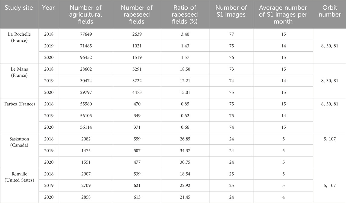
Table 1. The data sets used in this study. The location of these fields is shown in Figure 1.

2.2.3 Image preprocessing and dataset creation

Calibration of S1 images was conducted using the S1 toolbox developed by the European Space Agency (ESA). This calibration involved two steps: first, radiometric calibration, which converted digital numbers into linear backscatter coefficients (σ°), and second, geometric correction, where images were ortho-rectified using a 30 m digital elevation model from the Shuttle Radar Topography Mission (SRTM). The average S1 backscattering coefficient at the field scale was calculated using field boundary data. This was done by calculating the mean of pixel values within each field for each acquired S1 image. Subsequently, S1 time series were generated for each field at each rapeseed cultivation year, specifically 2018, 2019, and 2020. For classification, the backscatter coefficients (σ°) were used on a linear scale, while for dynamic backscatter analysis, the data were converted to decibels (dB), a logarithmic scale. Using the logarithmic scale (dB) makes the variations in backscattering dynamics more apparent.

The input data for our classifiers consisted of a 5-month S1 time series in VV and VH polarizations, capturing key stages of the rapeseed growth cycle, including stem elongation (approximately 30–40 days after germination, depending on the cultivation region), when the stem undergoes rapid vertical growth and thickening; inflorescence emergence (approximately 50–60 days after germination, depending on the cultivation region), marked by the appearance of flower buds at the top of the stem; flowering (approximately 60–70 days after germination, depending on the cultivation region), when an increase in the plant’s biomass and structural complexity leads to greater radar backscatter; and fruit development (approximately 70–80 days after germination, depending on the cultivation region), characterized by the formation and expansion of seed pods. A significant peak in S1 backscatter was observed during the inflorescence emergence and fruit development stages for both VV and VH polarizations. In fact, in a previous study, Maleki et al. (2024) highlighted that comparable results could be obtained by using both the entire growth cycle’s time series or a shorter time series covering only the aforementioned growth stages of rapeseed. The shorter time series reduced data storage requirements, streamlined downloads, and decreased the processing time.

Figure 2 shows the time series of S1 average backscatter coefficients for rapeseed fields in the five study sites over the 2018, 2019 and 2020 cultivation years. The study period is indicated by the dashed lines. During the initial portion of the study period, which includes the stem elongation, inflorescence emergence, and fruit development phases of rapeseed, both S1 VV and VH polarizations gradually increase, reaching a peak value. For the French study sites (Figures 2A–F), the S1 backscatter begins to rise in April, peaks between −12 and −10 dB for VH and −9 to −7 dB for VV in May. This peak is attributed to increased biomass, the height of rapeseed plants, and the random orientation of branches, which amplify backscatter through a double-bounce effect (Veloso et al., 2017; Mercier et al., 2019). Afterward, as senescence begins in June, backscatter declines, primarily due to reduced water content in the upper layers of rapeseed and an increased soil contribution to the S1 backscattering signal relative to vegetation. Therefore, our study period at the French sites included 2 months before and 1 month after this period to account for interannual variations (1 March - 1 August).

Figure 2

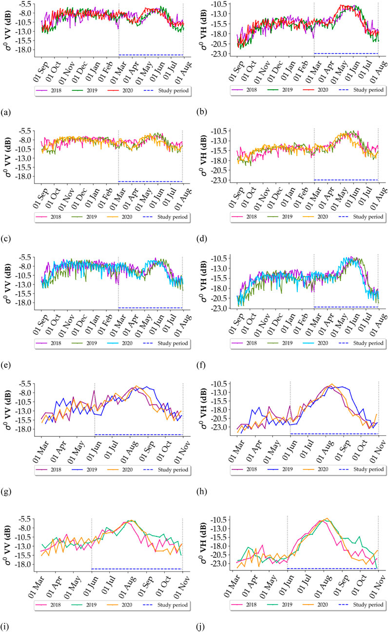
Figure 2. Time series of S1 average backscattering coefficients (σ°) in VV and VH polarizations for rapeseed fields in each year (2018, 2019 and 2020). The temporal period used in this study is represented by dashed lines. (A) La Rochelle (Fr): VV, (B) La Rochelle: VH, (C) Tarbes (Fr): VV, (D) Tarbes: VH, (E) Le Mans (Fr): VV, (F) Le Mans: VH, (G) Saskatoon (Canada): VV, (H) Saskatoon: VH, (I) Renville (United States): VV, (J) Renville: VH.

For the North American study sites (Figures 2G–J), S1 backscatter starts to increase in June, reaches a peak in early August—ranging from −11 to −10 dB for VH and −6 to −5 dB for VV—and subsequently decreases from late August to early October. Therefore, our study period at the North American sites was chosen to be between 1 June and 1 November.

In addition, Figures 2A–J show sometimes a temporal shift in the S1 time series (position of the highest peak) of rapeseed fields either between different years or among distinct study sites.

2.3 Algorithms

In this study we opted for the RF and InceptionTime classification algorithms due to their robustness and proven effectiveness in similar studies dealing with rapeseed classification (Belgiu and Drăguţ, 2016; Maleki et al., 2023). In our previous study (Maleki et al., 2023), we conducted a comprehensive evaluation of machine learning and deep learning models specifically for rapeseed mapping, with RF and InceptionTime yielding the best results. RF is a popular choice known for providing reliable classification outcomes in similar applications, making it a solid benchmark for accuracy comparison. InceptionTime also performed exceptionally well, achieving the highest accuracy and showing remarkable stability with a narrow range between its minimum and maximum accuracy metrics. However, InceptionTime requires considerably more computational resources during the training phase compared to the other classifiers.

The RF algorithm is a well-known ensemble learning technique that combines the results of multiple decision trees to improve accuracy and prevent overfitting (Inglada et al., 2015). InceptionTime is a convolutional-based deep learning algorithm that has achieved state-of-the art performance on time series classification tasks (Fawaz et al., 2020). This model is designed specifically for multivariate time series classification and consists of five separate Convolutional Neural Networks (CNNs), each comprising two residual blocks with three Inception modules per block. These Inception modules utilize multiple one-dimensional convolutional filters of varying lengths, allowing the model to capture features at multiple temporal scales. To minimize fluctuations in accuracy that might occur with a single network, an ensemble of networks with distinct weight initializations is employed. Additionally, shortcut connections between residual blocks facilitate direct gradient flow, effectively addressing the vanishing gradient issue often seen in deep networks (Fawaz et al., 2020).

While in many cases model performance can be enhanced through hyperparameter optimization, in the considered context of model transferability, where training and test data come from different distributions, conducting model hyperparameter optimization on a validation set made up solely of held-out training data might not ensure strong performance on the test data. Therefore, we deliberately opted for default parameter values which are usually calibrated in such a way to adapt well to more generic settings (Fawaz et al., 2020). For RF, we used the standard implementation provided in the Scikit-learn library with their built-in training optimization procedure and default hyperparameters (e.g., 100 trees in the forest and the Gini impurity splitting criterion). The InceptionTime approach is implemented in PyTorch using the default parameters defined by the authors in Fawaz et al. (2020). All the models have been implemented in Python. Our classification implementation codes can be found at github.com/cassiofragadantas/Colza_Classif.

For InceptionTime, training was performed via backpropagation of the cross-entropy loss (between predicted and true label) over 100 epochs with an Adam optimizer with learning rate 10^–5 and a weight decay of 10^–6. The model obtained at the end of the 100 epochs was employed at the inference stage. Although we recognize that this strategy might be prone to overfitting, performing early-stopping on a validation dataset would not be optimal due to our unsupervised transfer setting (i.e., no labeled data is available for the targeted test dataset) as explained previously.

2.4 Methodology

To address the challenges related to rapeseed fields mapping, we assessed three main scenarios. Figure 3A shows the flowchart of the method with several scenarios adopted in the study. A detailed description of each scenario is provided in the following subsections.

Figure 3

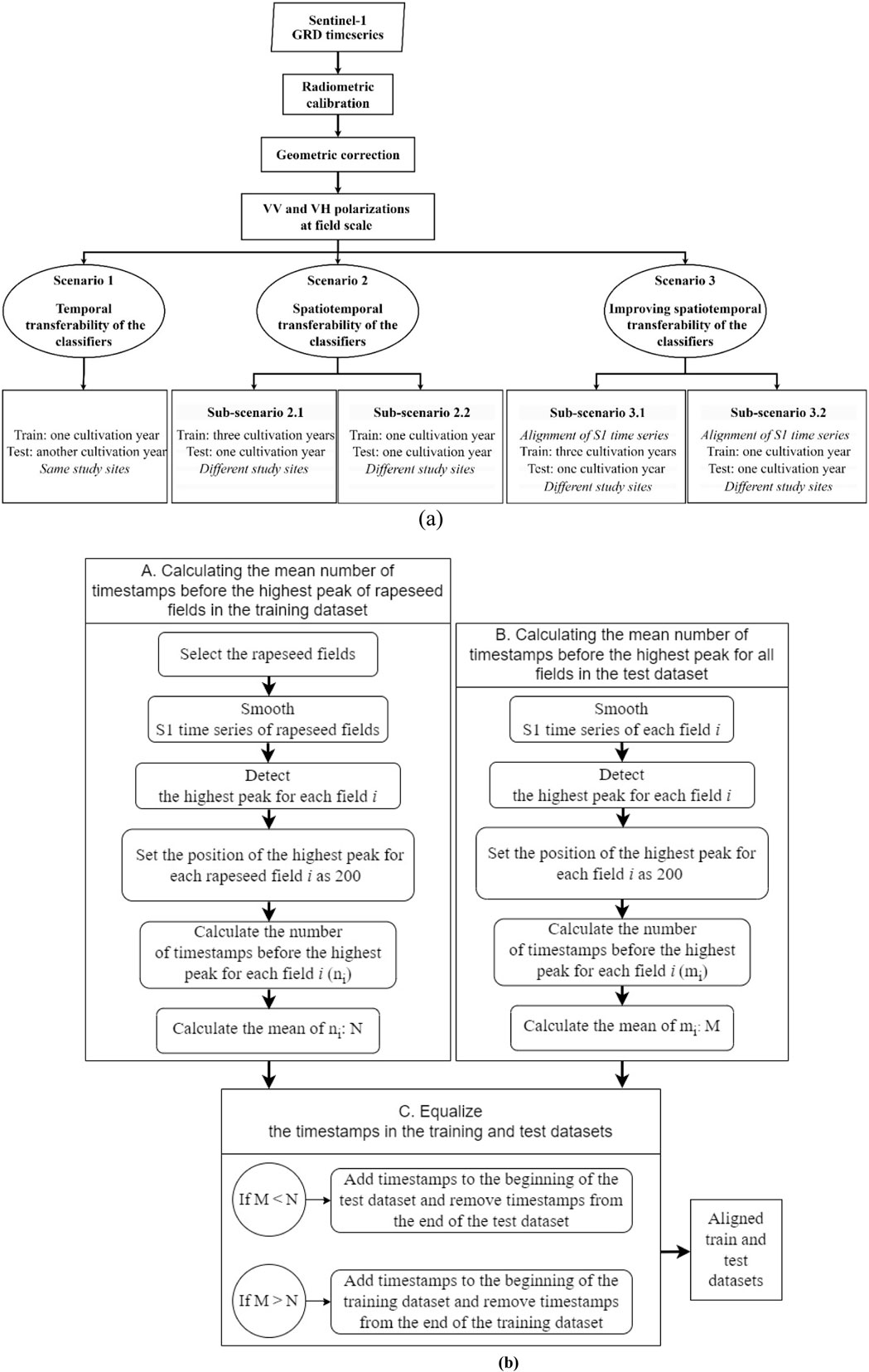
Figure 3. (A) Flow chart of the approaches that were tested in this study. (B) The flowchart of aligning S1 time series datasets based on the temporal position of the highest peaks of rapeseed fields.

2.4.1 Classification scenarios

2.4.1.1 Scenario 1: temporal transferability of the classifiers

In this scenario, the classifier (RF or InceptionTime) was trained using the S1 time series from 1 year within the 3 years of our study (2018, 2019, or 2020) to classify datasets from another year of the same study site. For instance, to generate the rapeseed map for Saskatoon in 2020, the training data from Saskatoon in 2018 or 2019 were employed. This evaluation encompassed testing 30 configurations, with 18 configurations for France and 12 for Canada-USA.

2.4.1.2 Scenario 2: spatiotemporal transferability of the classifiers

We evaluated the potential of rapeseed fields mapping using training and test data collected from different study sites within the same year (referred as spatial transferability of the classifiers), as well as from different study sites and cultivation years (considered both spatial and temporal transferability of the classifiers). To accomplish this, we used training data from one specific study site to classify data from another study site under similar climatic conditions. It is worth noting that rapeseed’s phenological cycle exhibits a maximum delay of 1 month between the study sites with similar climatic conditions (Maleki et al., 2023).

To assess this spatiotemporal transferability, we tested several combinations of datasets collected within each of our two climatic regions: the first climatic region encompassed French study sites (La Rochelle, Tarbes, Le Mans), while the second climatic region featured the two study sites in North America (Saskatoon in Canada, Renville in the United States).

We conducted this scenario according to two sub-scenarios.

2.4.1.2.1 Sub-scenario 2.1: three cultivation years training/one cultivation year test

In our first sub-scenario, we constructed a training dataset for each study site, consisting of S1 data from the 3 years 2018, 2019 and 2020. Each of these training datasets was then used to classify a single year’s dataset from another study site. For example, the La Rochelle training dataset with data from 2018, 2019 and 2020 was then used to classify the Tarbes datasets for 2018. This approach should enhance the classifiers robustness since it encompasses a greater variety of S1 backscattering coefficients for rapeseed, resulting from different meteorological conditions over 3 years, all of which affect the phenological cycle of rapeseed. This sub-scenario corresponds to the practical case where observations on a given site over many years are available and the objective is to carry out classification on a different site where no ground truth is available. This scenario involved testing 30 configurations of study sites and years (24 for France and 6 for Canada - United States).

2.4.1.2.2 Sub-scenario 2.2: one cultivation year training/one cultivation year test

In the second sub-scenario, classification was carried out considering a dataset from 1 year in the training site and a dataset from 1 year in the test site. In this paper, we presented four combinations of study sites. For the French study sites, the first combination involved La Rochelle as the training site and Tarbes as the test site, while the second combination used Tarbes as the training site and Le Mans as the test site (9 configurations of years for each combination). These site combinations showed more pronounced shifts in the phenological cycle between French study sites. In North America, the first combination consisted of Saskatoon as the training site and Renville as the test site, while the second combination was the reverse.

2.4.1.3 Scenario 3: improving spatiotemporal transferability of the classifiers by aligning S1 time series

In this section, we introduced an alignment method to improve the spatiotemporal transferability of the classifiers for rapeseed fields mapping. In scenario 3, both sub-scenarios of scenario 2 were repeated after applying the alignment method.

2.4.1.3.1 Sub-scenario 3.1: alignment of three cultivation years training/one cultivation year test

We used our novel alignment method to align the training dataset, which consisted of S1 time series from 3 years of one study site, with the test dataset, which consisted of a single year of data from another study site (with similar combinations of sites as described in sub-scenario 2.1). Classification was then performed on each pair of aligned training and test datasets.

2.4.1.3.2 Sub-scenario 3.2: alignment of one cultivation year training/one cultivation year test

The one-year training dataset was aligned with the one-year test dataset of different sites using alignment method (with similar combinations of sites and years as described in sub-scenario 2.2). Classification was then performed using each aligned training and test dataset.

2.4.1.4 Alignment method

In fact, the position of the highest peak in the S1 time series differs between 2 years or between two study sites as shown in Figure 2, which may likely induce lower accuracies when transferring a classifier from one site-year to another. The alignment of the highest peaks in the S1 time series of the training and test datasets was achieved through a process consisting of three steps outlined below (Figure 3B). The implementation codes are available at https://github.com/Saeideh-Maleki/Sentinel1-peak-alignement.

2.4.1.4.1 Calculating the mean number of timestamps before the highest peak of rapeseed fields in the training dataset

To align the highest peaks for rapeseed fields in S1 time series between training and test datasets, we started by performing the following procedures exclusively using the rapeseed fields in the training dataset:

• The highest peak for each rapeseed field within the training dataset was identified through a two-step process. Initially, the S1 time series of rapeseed fields were smoothed using a multidimensional Gaussian filter with a standard deviation equals to 4 days. Subsequently, the highest peak of S1 backscatter for each rapeseed field occurring during the peak period for rapeseed fields in the S1 time series was detected (between April 1st and July 1st for study sites in Europe, and between June 1st and November 1st for Canada and the United States sites). Supplementary Appendix Figure A1, provides a visual representation of these two steps for both VV and VH backscatter over a single rapeseed field.

• The position of the highest peak for each rapeseed field was standardized, arbitrarily setting it at 200 (Supplementary Appendix Figure A2). This number can be adjusted based on the number of timestamps in the time series. Subsequently, the number of timestamps (images) occurring before the highest peak for each rapeseed field i (n_i) was calculated, and the mean number of timestamps before the highest peak across all rapeseed fields in the training dataset (N) was computed.

2.4.1.4.2 Calculating the mean number of timestamps before the highest peak for all fields in the test dataset

The second step involved the identification of the highest peak for each field in the test dataset, whether it is rapeseed or not (operationally, we have no information about the crop types in the test datasets). First, the above-described multidimensional Gaussian smoothing process was performed on the test dataset, encompassing all fields, as shown in the Supplementary Appendix Figure A3. Subsequently, the position of the highest peak for each field was determined within the time frame where the potential rapeseed peak was logically expected to occur (between April 1st and July 1st for European study sites, and between June 1st and November 1st for sites in Canada and the United States).

The position of the highest peak for each field was then standardized by setting it to 200, as specified for the training dataset fields. This step is illustrated in the Supplementary Appendix Figure A4, showing the process for a single rapeseed field and a grassland field. The number of timestamps occurring before the highest peak for each field (m_i) was calculated, and subsequently, the mean number of timestamps before the highest peak for all fields was computed (M).

2.4.1.4.3 Equalize the number of timestamps in the training and test datasets

This final step consists in adding/removing timestamps in either the training or test dataset in order to align their peak positions. This was done in a way to maintain the initial number of timestamps, since RF and InceptionTime algorithms require homogeneous training and test sets in terms of input sample dimension.

For simplicity, we suppose that the average peak position in the test dataset is lower than in that of the training dataset, i.e., M < N.

For all fields in the test dataset with peak position (m_i) smaller than N:

1) Add (N-m_i) timestamps at the beginning of the test dataset by replicating its first timestamp (left padding) (Supplementary Appendix Figure A5).

2) Remove the same number of timestamps (N-m_i) from the end of the test dataset (right trimming) so that the peak is now at position N.

In the converse case (M > N), the roles of train and test datasets in the description above are switched. Figures 4, 5 illustrate the peak alignment procedure for the particular cases of M < N and M > N, respectively, presenting the average S1 time series for all rapeseed fields before (a, b) and after alignment (c, d).

Figure 4

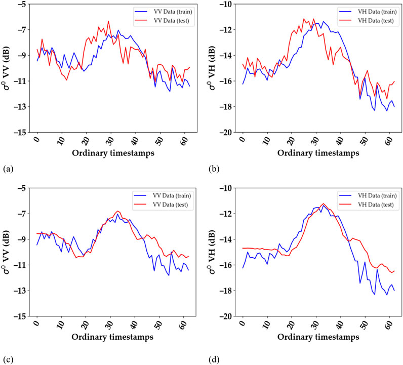
Figure 4. An example of alignment for M < N: Average S1 time series of all rapeseed fields before (A, B) and after alignment (C, D). Training dataset = La Rochelle 2018, 2019, and 2020; test dataset = Tarbes 2020. (A, C): VV polarization, (B, D) VH polarization. The graph corresponding to the test dataset appears smoother after alignment due to the use of a different number of duplicated timestamps for each field. However, the shape of the graph for a single field remains unchanged, with a slight temporal shift (equal to the duplicated timestamps). Ordinary timestamps indicate the sequential order of images in the time series, starting from 0 (representing the first image) and increasing by 1 for each subsequent image.

Figure 5

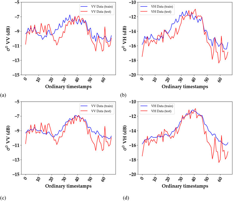
Figure 5. An example of alignment for M > N: Average S1 time series of all rapeseed fields before (A, B) and after alignment (C, D). Training dataset = Tarbes 2018, 2019, and 2020; test dataset = La Rochelle 2018. (A, C): VV polarization, (B, D) VH polarization. The graph corresponding to the training dataset appears smoother after alignment due to the use of a different number of duplicated timestamps for each field. However, the shape of the graph for a single field remains unchanged, with a slight temporal shift (equal to the duplicated timestamps). Ordinary timestamps indicate the sequential order of images in the time series, starting from 0 (representing the first image) and increasing by 1 for each subsequent image.

It is important finally to note that since the peak was detected within a constrained time window (comprising the period with the highest SAR backscatter coefficient for rapeseed in the study area), the number of duplicates (padding) was limited, with an average of only five duplicates in a time series consisting of 65 images. Furthermore, the duplicated data were in the early part of the time series, unrelated to the main peak period, thus avoiding any negative impact on the classification process. Importantly, the smoothing process was only applied during the highest peak detection phase, and both the training and test datasets remained unsmoothed when timestamps were added or removed.

Summary of the peak alignment procedure.

- Compute the average peak position in the training dataset (considering rapeseed fields only) and test dataset (considering all fields), as described in steps A and B.

- For the dataset with the smaller average peak position, perform left padding (and the corresponding right trimming) on each field so that their peak position matches the other dataset’s average peak position, as described in step C.

2.4.2 Evaluation metrics

To assess the performance of the different classification approaches, we evaluated the following metrics on the test dataset: precision, recall, F1 score and Kappa coefficient (Equations 1–4 respectively). Given the highly imbalanced nature of the considered datasets (small proportion of positive samples) a simple measure of accuracy would not be informative, while the precision-recall measures are better adapted to this context.

$\text{Recall}=\frac{TP}{TP+FN}(1)$

$\text{Precision}=\frac{TP}{TP+FP}(2)$

$\mathrm{F}1=\frac{2*\left(Precision*Recall\right)}{Precision+Recall}(3)$

$\text{Kappa}=\frac{Po-Pe}{1-pe}(4)$

• True positives (TP) represent the number of fields correctly identified as rapeseed.

• False positives (FP) represent the number of non-rapeseed fields classified as rapeseed.

• False negatives (FN) represent the number of rapeseed fields misclassified as non-rapeseed.

• Observed agreement ($\left.Po\right)$: The proportion of agreement between two raters or methods based on the actual observed data. It is calculated as the sum of true positives and true negatives divided by the total number of instances (Chicco et al., 2021).

• Expected agreement $\left(Pe\right)$: The expected agreement that occurs by chance. It is calculated based on the marginal probabilities of agreement for positive and negative instances (Chicco et al., 2021).

3 Results

3.1 Scenario 1: temporal transferability of the classifiers

The results of the accuracy assessment for temporal transferability using the RF and InceptionTime methods are shown in Table 2. The accuracy metrics for each study site are presented as the average value (Mean), the highest (Max) and lowest (Min) calculated from the six combinations of training and testing years (for each site, 2018–2019, 2018–2020, 2019–2018, 2019–2020, 2020–2018, 2020–2019, the first year for training and the second year for testing).

Table 2

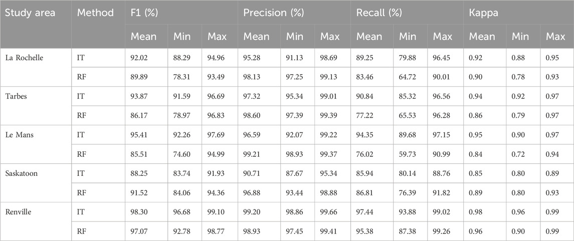
Table 2. Scenario 1: Accuracy assessment of temporal transferability of the classifiers created by InceptionTimes and RF algorithms in five study sites (La Rochelle, Tarbes, Le Mans, Saskatoon, Renville). ‘Mean’, ‘Max’, and ‘Min’ represent respectively the average value, the highest value, and the lowest value of each metric across all combinations of years.

According to Table 2, the mean F1 and Kappa scores achieved by the RF algorithm were consistently above 85.5% and 0.84, respectively. When using the InceptionTime algorithm, the mean F1 and Kappa scores exceeded 88.2% and 0.85, respectively. An average precision of over 90% indicates that both RF and InceptionTime have a remarkable ability to correctly label rapeseed fields while minimizing false positives while an average recall of over 75%, indicates that the classifiers were able to identify a significant number of rapeseed fields.

The results in Table 2 demonstrates that using the S1 time series of flowering and harvest (period showing the rapeseed characteristic peak) allows both RF and InceptionTime to generate accurate rapeseed maps across all study sites through the temporal transferability of the classifiers. However, a comparison of F1 scores between RF and InceptionTime shows that InceptionTime has a narrower value range between minimum and maximum F1 scores.

3.2 Scenario 2: spatiotemporal transferability of the classifiers

3.2.1 Sub-scenario 2.1: three cultivation years training/one cultivation year test

This scenario included a training dataset composed of 3 years’ time-series applied to one-year test time series of another site sharing similar climatic conditions as the training site. The accuracy metrics of this scenario are summarized in Table 3, where the Mean, Max and Min correspond respectively to the average value, the highest value and the lowest value of each accuracy metric across all three test years (2018, 2019, 2020). Using the RF, the mean F1 scores ranged between 82.7% and 97.8% and the mean Kappa scores between 0.8 and 1.0 across all testing sites/years. Slightly higher values are also obtained using the InceptionTime with F1 scores ranging from 88.7% to 97.1%, and mean Kappa scores in the range of 0.9–1.0. Examining the precision and recall, the RF algorithm achieved mean precision and recall scores greater than 89.0% and 75.0% respectively, whereas for InceptionTime algorithm the mean precision and recall were both higher than 85%.

Table 3

Table 3. Scenario 2, sub-scenario 2.1: Accuracy of rapeseed fields detection using spatiotemporal transferability of the classifiers created by RF and InceptionTime (IT) algorithms. Evaluation was conducted for six site combinations in France (La Rochelle–Le Mans, Le Mans–La Rochelle, Le Mans–Tarbes, Tarbes–Le Mans, Tarbes–La Rochelle, La Rochelle–Tarbes), and two site combinations in North America (Saskatoon in Canada–Renville in United States, Renville–Saskatoon). Mean, Max, and Min represent the average, highest, and lowest values of each accuracy metric across all 3 years.

3.2.2 Sub-scenario 2.2: one cultivation year training/one cultivation year test

The results of classification in this sub-scenario of spatiotemporal transferability using 1 year training data from one study site and 1 year test data from another site, can be found in Table 4 for La Rochelle (LR) – Tarbes (TA) and Tarbes–Le Mans (LM), and in Table 5 for Saskatoon (SA) – Renville (RE) and Renville–Saskatoon. When using one-year datasets for both training and testing for the two combinations of French study sites (Table 4), the RF achieves F1 scores ranging from 48.8% to 97.7%. While the InceptionTime algorithm yields F1 scores from 59.2% to 97.7%. In Table 5, focusing on the North American study sites, the F1 scores using the RF classifier vary from 49.0% to 96.6%, while InceptionTime algorithm produces F1 scores within the range of 58.4%–94.2%.

Table 4

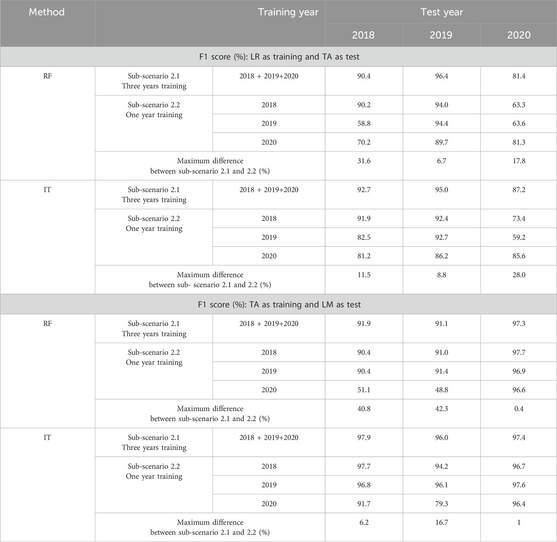
Table 4. Scenario 2, sub-scenarios 2.1 and 2.2 (France): Comparison between F1 scores (%) obtained from the three-year training dataset (sub-scenario 2.1) and the one-year training dataset (sub-scenario 2.2) for two combinations of French study sites: La Rochelle (LR) site as training and Tarbes (TA) as test, Tarbes (TA) as training and Le Mans (LM) as test. The maximum difference represents the maximum difference between the F1 score obtained from sub-scenario 2.1 and the three F1 scores obtained from sub-scenario 2.2.

Table 5

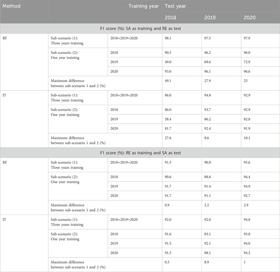
Table 5. Scenario 2, sub-scenarios 2.1 and 2.2 (North America): Comparison of F1 scores (%) using the three-years training dataset (sub -scenario 2.1) and the single-year training dataset (sub-scenario 2.2) for two combinations of North American study sites: Saskatoon (SA) as the training set and Renville (RE) as the test set, and vice versa. Maximum difference represents the greatest difference between the F1 score obtained from sub-scenario 2.1 and the three F1 scores derived from sub-scenario 2.

3.2.3 Comparison between the two sub-scenarios of spatiotemporal transferability

Tables 4, 5 also include the results obtained on the sub-scenario 2.1 alongside with the ones obtained on sub-scenario 2.2, to allow a comparison between both sub-scenarios. Comparing the results of the two sub-scenarios for La Rochelle–Tarbes, Table 4 shows that using La Rochelle’s 3 years training data for classifying Tarbes 2018, the maximum F1 score improvement is 31.6% with RF (compared to La Rochelle 2019 as training and Tarbes 2018 as test) and 11.5% with InceptionTime (compared to La Rochelle 2020 as training and Tarbes 2018 as test). For the classification of Tarbes 2019, the maximum F1 improvement is 6.7% with RF and 8.8% with InceptionTime (compared to La Rochelle 2020 as training and Tarbes 2019 as test for both algorithms). Tarbes 2020 achieves a maximum F1 score increase of 17.8% with RF (compared to La Rochelle 2018 as training and Tarbes 2020 as test) and 28.0% with InceptionTime when using the classifier with multi-date data (compared to La Rochelle 2019 as training and Tarbes 2020 as test).

In the case of Tarbes–Le Mans (Table 4), creating the rapeseed map for Le Mans 2018 using Tarbes’s three-year training data results in a maximum F1 score improvement of 40.8% with RF, and 6.2% with InceptionTime (compared to Tarbes 2020 as training and Le Mans 2018 as test for both algorithms). For Le Mans 2019, the maximum F1 score improvements are 42.3% with RF and 16.7% with InceptionTime (compared to Tarbes 2020 as training and Le Mans 2019 as test for both algorithms). The results of rapeseed detection of Tarbes 2020 show a maximum F1 score improvement of 0.7% with RF and 1.0% with InceptionTime (compared to Tarbes 2020 as training and Le Mans 2020 as test for both algorithms) when using the classifier with multi-date data.

Creating the rapeseed map for Renville 2018 using Saskatoon’s multi-year training data (Table 5) resulted in a maximum F1 score increase of 49.1% with RF and 27.6% with InceptionTime (compared to Saskatoon 2019 as training and Renville 2018 as test for both algorithms). For Renville 2019, using multi-year data for training led to maximum F1 score improvements of 27.9% with RF and 8.6% with InceptionTime (compared to Saskatoon 2019 as training and Renville 2019 as test for both algorithms). In the case of Renville 2020, the use of multi-year data resulted in maximum F1 score enhancements of 25% with RF and 10.1% with InceptionTime (compared to Saskatoon 2019 as training and Renville 2020 as test for both algorithms). The results for creating the rapeseed map for Saskatoon using Renville’s multi-year training data showed only a slight increase in the F1 score compared to the one-year Sub-scenario.

3.3 Scenario 3: improving spatiotemporal transferability of the classifiers by aligning S1 time series

In this scenario, the spatial and temporal transferability analysis previously conducted in Section 3.2 (the previous section) was repeated by employing the alignment method for training and test datasets.

3.3.1 Sub-scenario 3.1: alignment of three cultivation years training/one cultivation year test

The comparison of F1 scores of our first sub-scenario (three-years training/one-year test) before and after alignment using RF and InceptionTime algorithms is presented in Table 6 for all combinations of study sites and years in France, and Table 7 for all combinations of study sites and years in North America. For the French sites (Table7), the most notable improvement was observed when aligning the datasets from Le Mans (3 years) as the training dataset and Tarbes (2020) as the test dataset, resulting in a 9.9% increase in F1 score (from 77.9% before alignment to 87.8% after alignment using RF). Similarly, aligning the datasets from La Rochelle (3 years) as training and Tarbes (2020) as test resulted in an 8.0% improvement in F1 score (from 81.5% before alignment to 89.5% after alignment using RF). Figures 2A–F which illustrate the S1 time series of rapeseed backscatter at the French study sites, clearly show the temporal shifts between the phenological cycle of 3 years of Le Mans and Tarbes in 2020, and between the 3 years of La Rochelle and Tarbes in 2020. Thus, aligning the position of the highest peak in the S1 time series led to significant improvements in F1 scores, particularly in cases where the temporal shift was most pronounced. In North America (Table 7), alignment also improved the results of classification using RF and InceptionTime. The highest improvement occurred when aligning the dataset of the United States (3 years) as training and Canada (2020) as the test, resulting in a 3.2% increase in F1 score (from 89.1% before alignment to 92.3% after alignment using RF). Overall, it’s worth noting that the improvement in North America was less pronounced compared to the results in France.

Table 6

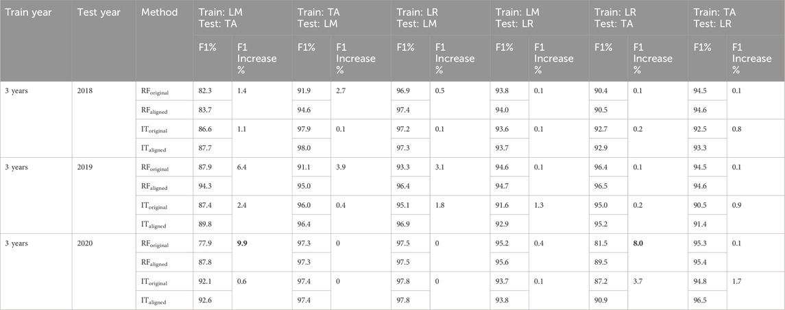
Table 6. Scenario 3, sub-scenario 3.1 (France): Comparison of F1 scores (%) before and after alignment of training and test datasets (3 years training and one-year test) for study sites in France (LR = La Rochelle, TA = Tarbes, LM = Le Mans). The “F1 increase” represents the difference between the F1 score after and before the alignment of the training and test datasets. The two highest increases in F1 are shown in bold. RF_original: RF using the datasets before alignment, RF_aligned: RF using the data sets after alignment, IT_original: InceptionTime using the data sets before alignment, IT_aligned: InceptionTime using the data sets after alignment.

Table 7

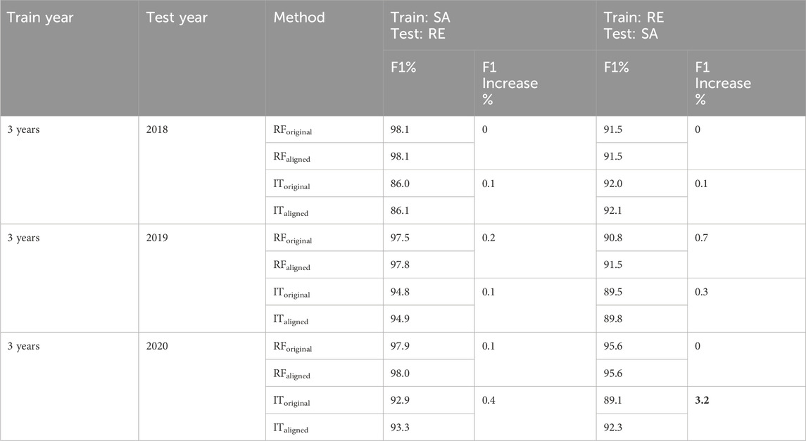
Table 7. Scenario 3, sub-scenario 3.1 (North America): Comparison of F1 scores (%) before and after alignment of training and test datasets (3 years training and 1 year test) for study sites in North America (Saskatoon = SA, Renville = RE). The “F1 increase” represents the difference between the F1 score after and before the alignment of the training and test datasets. The highest increase in F1 is shown in bold. RF_original: RF using the datasets before alignment, RF_aligned: RF using the data sets after alignment, IT_original: InceptionTime using the data sets before alignment, IT_aligned: InceptionTime using the data sets after alignment.

3.3.2 Sub-scenario 3.2: alignment of one cultivation year training/one cultivation year test

Table 8 presents a comparison of F1 scores for the second sub-scenario, which includes one-year training and one-year testing, both before and after applying the alignment method with the RF and the InceptionTime algorithms. This analysis focused on two combinations of French study sites, namely, La Rochelle–Tarbes and Tarbes–Le Mans. Meanwhile, Table 9 provides the corresponding results for two combinations of North American study sites: Saskatoon–Renville, and Renville–Saskatoon.

Table 8

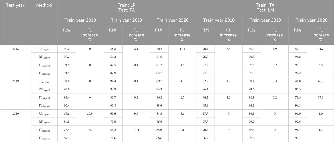
Table 8. Scenario 3, sub-scenario 3.2 (France). Comparison of F1 scores (%) before and after alignment of training and test datasets (one-year training and one-year test) for two combinations of study sites in France: La Rochelle as training/Tarbes as test (LR/TA), Tarbes as training/Le Mans as test (TA/LM). “F1 increase” represents the difference between the F1 value before and after the training and test data sets were aligned. The two highest F1 increases are shown in bold. RF_original: RF using the data sets before alignment, RF_aligned: RF using the data sets after alignment, IT_original: InceptionTime using the data sets before alignment, IT_aligned: InceptionTime using the data sets after alignment.

Table 9

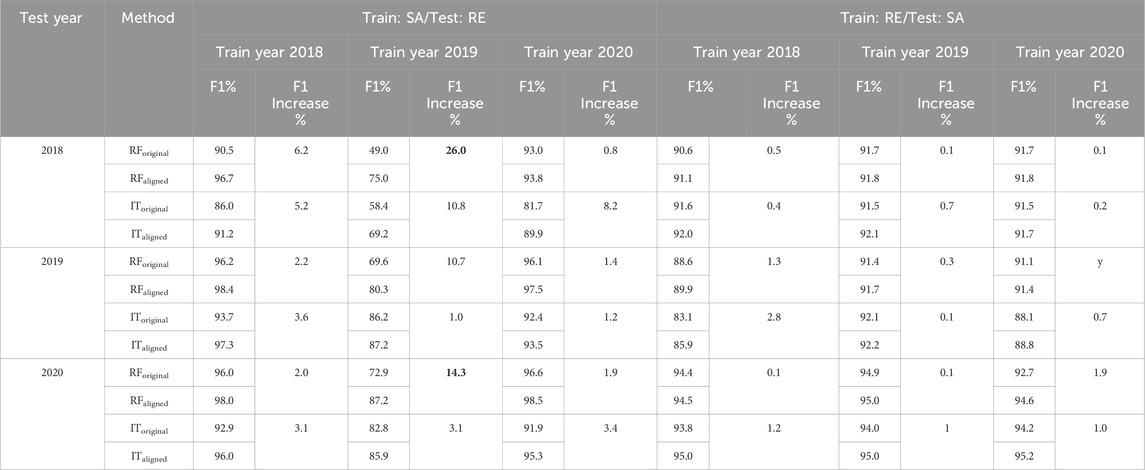
Table 9. Scenario 3, sub-scenario 3.2 (North America). Comparison of F1 scores (%) before and after alignment of training and test datasets (one-year training and one-year test) for study sites in North America (Saskatoon = SA, Renville = RE). “F1 increase” represents the difference between the F1 value before and after the training and test data sets were aligned. The two highest F1 increases are shown in bold. RF_original: RF using the data sets before alignment, RF_aligned: RF using the data sets after alignment, IT_original: InceptionTime using the data sets before alignment, IT_aligned: InceptionTime using the data sets after alignment.

For the French study sites, Table 8 clearly demonstrates that time series alignment significantly enhances F1 scores when using both RF and InceptionTime. The most remarkable improvements among the results of both algorithms, were observed when aligning the datasets of Tarbes (2020) for training and Le Mans (2019) for testing, resulting in a 46.7% increase in F1 score (from 48.8% before alignment to 95.5% after alignment using RF). Similarly, aligning the datasets of Tarbes (2020) for training and Le Mans (2018) for testing led to an increase of 44.7% in F1 score (from 51.1% before alignment to 95.8% after alignment using RF).

In North America, as shown in Table 9, the most significant enhancements occurred when aligning the datasets of Saskatoon (2019) for training and Renville (2018) for testing, resulting in a 26.0% increase in F1 score (from 49.0% before alignment to 75.0% after alignment using RF). Similarly, aligning the datasets of Saskatoon (2019) and Renville (2020) resulted in a 14.3% increase in F1 score (from 72.9% before alignment to 87.2% after alignment using RF).

3.3.3 Comparison between the two sub-scenarios of improving spatiotemporal transferability

Comparing the results between the two sub-scenarios (three-year training/one-year test in Tables 6, 7 and one-year training/one-year test in Tables 8, 9) reveals that the most substantial improvement is observed in the second sub-scenario (1 year as the training period). Specifically, the one-year training sub-scenario experiences the highest improvement of 46.7%, in contrast to the three-year training sub-scenario, which shows the highest improvement of 9.9%. Notably, before alignment, the three-year training sub-scenario outperformed the one-year training sub-scenario, which may explain the relatively lower improvement observed in the results of the three-year sub-scenario after alignment.

3.4 The rapeseed fields map

Figure 6 presents a comparison of rapeseed fields maps for a specific case, where Tarbes 2020 serves as the training dataset, and Le Mans 2019 as the test dataset. These maps show both before (Figures 6A, B using RF and InceptionTime, respectively) and after applying our alignment method (Figures 6C, D using RF and InceptionTime, respectively) to the S1 time series. The comparison is made against the ground samples of rapeseed fields. In these figures, the correctly classified rapeseed fields (True positives) are colored in green. In contrast, rapeseed fields incorrectly classified as non-rapeseed (False negatives) are indicated by empty red polygon outlines. It is worth noting that the percentage of non-rapeseed fields misclassified as rapeseed (False positives), marked in orange, is very low, at just 1%, making it a rare occurrence.

Figure 6

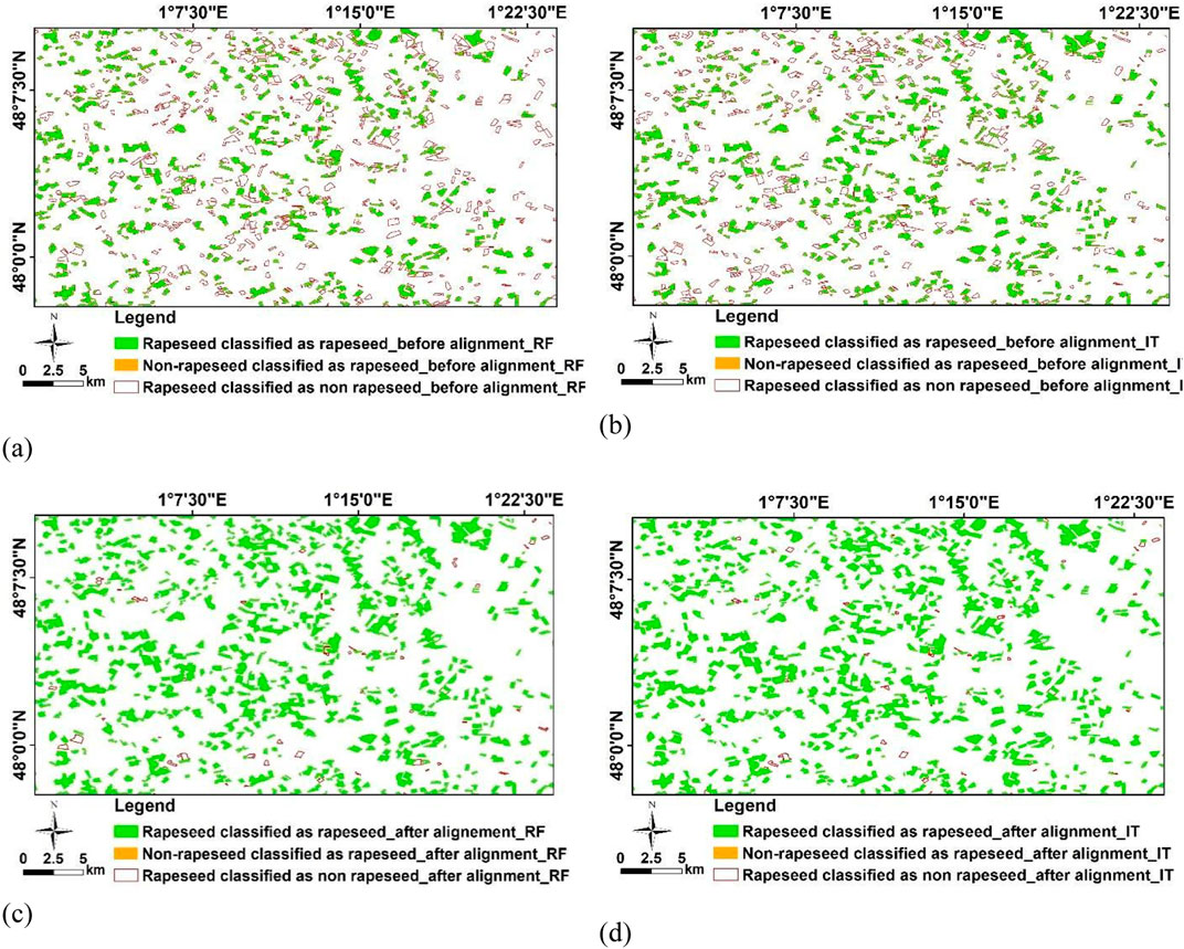
Figure 6. Comparing the rapeseed fields maps of Tarbes 2020 as training and Le Mans 2019 as test before and after applying our alignment approach of S1 time series. (A) Using RF before alignment method, (B) using InceptionTime (IT) before alignment method, (C) using RF after alignment method, (D) using InceptionTime after alignment method. The percentage of non-rapeseed fields that are misclassified as rapeseed, shown in orange, is very low, at only 1%, which makes it a rare occurrence.

As observed in Figures 6A, B, before aligning the S1 time series, many rapeseed fields sampled from the ground (RPG) were incorrectly classified as non-rapeseed. However, Figure 6B demonstrates that InceptionTime outperforms RF in correctly identifying rapeseed fields. On the other hand, Figures 6C, D provide a view of spatiotemporal transferability of the classifiers after applying our alignment method. These figures highlight the high performance of the alignment method in the spatiotemporal transfer for rapeseed classification. After alignment, misclassifications primarily involve small-sized rapeseed fields. This problem is due to the reduced number of S1 pixels used in the calculation of the average backscatter coefficient, which compounds the speckle effect. It is important to note that this type of error, particularly in the case of smaller-sized rapeseed fields, is not a direct consequence of the method employed but rather is linked to the spatial resolution of S1 images.

4 Discussion

This paper addresses several challenges associated with rapeseed fields mapping to improve the detection of this crop, particularly when collecting new training data is limited. We proposed a comprehensive approach to handling the complexities of field data collection and the transferability of the classifiers. Our approach is particularly relevant as there is a growing demand for crop monitoring at a national or global scale, while the availability of ground data across different regions and time frames remains a significant challenge, as highlighted by various studies (Johnson and Mueller, 2021; Henits et al., 2022; Lin et al., 2022).

4.1 Temporal transferability of the classifier

The results of temporal transferability of classifiers illustrated that, in all five study sites, both RF and InceptionTime algorithms consistently achieved high accuracy when classifying rapeseed fields from 1 year using the training dataset from another year (F1 and Kappa scores consistently exceeded 85% and 0.84) (Table 2). These high accuracy levels show that across all our five study sites, the classifiers have the ability to effectively distinguish rapeseed fields using training data from different years. The InceptionTime model used in this study achieved an F1 score of over 90% using only S1 time series, outperforming previous methods for classifying time series data. Maleki et al. (2023) used S1 time series for rapeseed mapping and examined temporal transferability for this task using RF, MLP, LSTM-FCN, and InceptionTime models. They achieved the highest mean F1 score with InceptionTime (92.7%). In another study, Rusňák et al. (2023) applied temporal transferability using SVM and a neural network (NN) algorithm to map seven crops—barley, rapeseed, maize, wheat, sugar beet, sunflower, and soybean—achieving overall accuracy ranging from 84.4% to 88.9% with the SVM algorithm and from 81.1% to 91.9% with the NN algorithm. Pandžić et al. (2024) achieved an overall F1 score ranging from 78% to 88% for mapping nine crops using RF and Convolutional Neural Network algorithms, based on highly dense time series data from S1. Lin et al. (2022) employed a historical threshold approach on S2 and Landsat data, achieving F1 scores between 85% and 87% for detecting various crops. Additionally, the InceptionTime model, which directly learns crop backscatter patterns from satellite imagery, offers a simpler alternative to decision boundary-based approaches (Yaramasu et al., 2020; You and Dong, 2020). In contrast, threshold-based methods rely on selecting crop-specific thresholds from historical samples to apply to a target year.

Notably, InceptionTime achieved an F1 score higher than 90% in four study sites (La Rochelle, Tarbes, Le Mans, Renville), while the RF algorithm reached an F1 score higher than 90% in one study site (Renville). InceptionTime also displayed a narrower range between minimum and maximum F1 scores when compared to RF, demonstrating greater stability in classification accuracy. Fawaz et al. (2020) showed that InceptionTime has less variation in accuracy thanks to its architecture composed of a series of convolutional layers with filters of varying lengths combined with residual connections. This suggests that InceptionTime is well suited for rapeseed fields classification in a temporal transferability context, providing consistent performance across different years. Transfer learning leverages shared patterns or characteristics that exist across different domains or datasets. For rapeseed, many of these characteristics are tied to growth stages and phenological changes that produce distinguishable patterns in satellite data. These patterns allow the classifier to transfer a model trained on one dataset to another (Nowakowski et al., 2021).

4.2 Spatiotemporal transferability of the classifier

In the sub-scenario where 3 years of data from one study site were used for training and 1 year of data from another study site were used for testing, both the RF and InceptionTime algorithms demonstrated strong spatiotemporal transferability (Table 3). The mean F1 scores of RF ranged from 82.7% to 97.8%, with mean Kappa scores consistently between 0.8 and 1. The InceptionTime algorithm achieved mean F1 scores ranging from 88.7% to 97.1%, with mean Kappa scores between 0.9 and 1. In a study by Mercier et al. (2020), an incremental method developed by Mercier et al. (2019) was adopted to detect rapeseed fields using only S1 time series from the same training and test sites, resulting in a lower accuracy with a kappa value of 0.63. (Sun et al., 2024). tested 12 models on rapeseed field detection, combining three convolutional neural network (CNN) models (U-Net, PSPNet, and DeepLab V3) with four backbone networks (ResNet-18, ResNet-34, ResNet-50, and ResNet-101). PSPNet outperformed the others, achieving an F1 score of 93.3% for same-year train-test scenarios. Previous studies on rapeseed detection have often relied on optical images alone or a combination of radar and optical images to achieve high accuracy (Mouret et al., 2021; Woźniak et al., 2022). For instance, Han et al. (2021a) achieved F1 scores ranging from 0.84 to 0.91 by combining S1 and S2 data to map rapeseed fields across 33 countries using a pixel- and phenology-based method. Compared with previous studies, both algorithms considered in this study are effective in classifying S1 data from different sites for training and testing. However, a narrower range between the minimum and maximum values of F1 scores is obtained by InceptionTime, indicating a higher stability of this algorithm in the transfer domain.

In the sub-scenario where one-year data from a specific study site was used for training and another one-year dataset from a different study site was used for testing, although high F1 scores were achieved for certain combinations (e.g., F1 of 96.6% for Canada 2019-USA 2019), both RF and InceptionTime algorithms showed high variation between the minimum and maximum F1 scores within the various combinations of study sites (Tables 4, 5). F1 scores ranged from 48.8% to 97.7% with RF and from 59.2% to 97.7% with InceptionTime in France study sites (Table 4). In North American cases, F1 scores using RF ranged from 49.0% to 96.6%, while InceptionTime yielded scores between 58.4% and 94.2% (Table 5). Previous studies using spatiotemporal transferability of classifier for crop mapping have also reported a wide range of accuracy results. Belgiu et al. (2021) achieved an overall accuracy ranging from 69% to 75% for 10 crops when applying spatiotemporal transferability within two study sites in the Netherlands using S2 time series and the RF algorithm. Meanwhile, Luo et al. (2022) used training data from England and France to produce crop maps for ten European countries and reported an overall accuracy of 89% in crop classification using S2 time series.

Comparing the results of our two spatiotemporal transfer sub-scenarios (Tables 3–5), the use of multi-year training data resulted in smaller variations in classification performance across different combinations of sites. Cai et al. (2022), who used a 15-year Landsat dataset to create a crop map for 2015 across the US, showed that a larger training dataset can significantly improve the classification performance. However, they also found that adding more years beyond a certain range can lead to a plateau in performance improvement.

Also, our results showed significant improvements in F1 score when training on data from multiple years, with the most notable enhancements observed with RF. Thus, training with multi-year backscatter data is beneficial, in order to improve the accuracy of classification using the spatiotemporal transferability of classifier while minimizing the difference between minimum and maximum accuracy. These results suggest that the use of multi-year training data, representing various phenology cycles and environmental conditions, enhance the accuracy and reliability of classification models mainly for the transferability of the classifiers when the labeled data are rare. As previous studies have mentioned that the lack of ground data poses a significant challenge to supervised classification methods over large study sites (Burke et al., 2021; Nowakowski et al., 2021), our approach of transferring models trained in one region to map larger spatial extents is of great value.

4.3 Improving spatiotemporal transferability of the classifier

Comparing the efficacy of the proposed alignment method between 3 years training and one-year training sub-scenarios showed that the alignment method induces significant improvement for one-year training cases and limited improvement for the three-years training. These results were expected since the three-years training included vast variation in the S1 time series data among the 3 years allowing the classification model to account for most of the possible cases in the training phase. For this reason, it achieves a high F1 before applying the alignment method. However, using one-year training dataset, the ability of the trained model to account for changes in the S1 time series between years was limited. Practically, the case of having 1 year of training data is more likely to occur in operational mapping, which highlights the significance of the proposed alignment method.

To discuss the impact of time series alignment on F1 score enhancement, we compared between the percentage of improvement in the F1-score after alignment and the temporal shift in the rapeseed peak for the S1 time series (in days), between the training and test datasets. This comparison is presented in the Supplementary Appendix Figures A6A, B (from Tables 6, 7) for the three-year training sub-scenario and in the Supplementary Appendix Figures A7A, B (from Tables 8, 9) for the one-year training sub-scenario. In these figures, the x-axis represents the temporal shift, i.e., the difference between the date of the highest peak in the training and test datasets. Both figures illustrate that, as the temporal shift between the highest peak of rapeseed in the training and test data increases, more improvement in F1 score after the application of the alignment method is observed.

However, some low improvement cases are mainly related to the results of the InceptionTime algorithm, showing that the improvement achieved through the alignment with InceptionTime may not be completely determined by the temporal shift between training and test datasets. For instance, for two cases in the Supplementary Appendix Figure A6A with more than 20 days’ shift, classifying Tarbes 2020 with a three-year training dataset of Le Mans showed an improvement of 0.6% using InceptionTime and 10% using RF (Table 6). Additionally, a similar situation is present for rapeseed detection in Le Mans 2019 with a three-year training dataset from Tarbes, leading to an improvement of 0.4% using the InceptionTime algorithm and 4% using RF (Table 6). Similarly, in the Supplementary Appendix Figure A7A, in the case of Tarbes 2020 – Le Mans 2018, with a temporal shift of 29 days, the InceptionTime presented a 5.5% improvement, while RF demonstrated a significant improvement of 44.7%. Furthermore, comparing the F1 scores of the RF and InceptionTime algorithms shows that peak alignment has a more pronounced effect on RF compared to InceptionTime which already achieved higher F1 scores (Tables 8, 9). These differences between the results of RF and InceptionTime may be attributed to the structural disparities between these two algorithms. Unlike RF, which builds independent decision trees that does not account for the temporal dependency between features, InceptionTime is a time series classification algorithm employing convolutional neural networks (CNN). It is specifically designed to handle time series data and it uses convolutional layers to extract meaningful features by sliding filters over the data (Fawaz et al., 2020). This enables InceptionTime to be on one hand robust to possible temporal shifts and on the other hand to capture temporal patterns, transitions, and dependencies within the time series, making it particularly advantageous for sequential data like S1 time series (Fawaz et al., 2020).

4.4 Factors affecting the time series alignment method

For some train/test combinations, the F1 score of the RF remains below 90% although there is an improvement in performance after alignment. For instance, for Le Mans 3 years - Tarbes 2020, the F1 score by RF increases from 77.9% to 87.8% after alignment (Table 6). Notably, as shown in the Supplementary Appendix Figure A8, for this combination a sudden decline in the S1 backscatter for Tarbes is present by the end of June 2020, creating a dissimilarity in the backscatter trend between the training and test data. However, this decline is not reflected in the S1 backscatter data for Tarbes in 2018 and 2019 (as shown in Figure 2, S1 backscatter for our study sites). A comparison of precipitation data for Tarbes between 2018, 2019 and 2020 shows a significant decrease in precipitation in 2020, especially between May and July. Precipitation in 2020 decreased by 47.1% compared to 2018 and by 74.5% compared to 2019. Therefore, low F1 value even after the alignment can be related to the meteorological variability in the study site, as this variability may change the SAR backscatter trend (Fieuzal et al., 2013; Han et al., 2021a). Shorachi et al. (2022) demonstrated that drought conditions lead to lower VV and VH backscatter values. Reduced VV and VH backscatter during drought periods may be attributed to factors such as dry soils, lower vegetation water content (VWC), and altered leaf geometry. The extent of these changes, however, varies depending on crop type, soil characteristics, and regional water management practices (for example, irrigation). The unusual S1 backscatter patterns, resulting from drought conditions, complicated the alignment between the training and test time series. Cai et al. (2022) observed that spatiotemporal transfer performance can produce outliers during extreme climatic events, such as droughts or unusually high precipitation years. Similarly, Rusňák et al. (2023) found that intense drought events in specific years pose significant challenges for spatiotemporal transfer.

5 Conclusion

This study explores the spatiotemporal transferability of RF and InceptionTime as a solution for limited availability of reference label data to map rapeseed fields. In addition, the paper introduced an approach that improve the rapeseed fields mapping through spatiotemporal transfer.

The performance of the RF and InceptionTime classifiers across different years in five diverse study sites was evaluated. Both algorithms consistently demonstrated strong performance, achieving high accuracy in classifying rapeseed fields using training data from 1 year and testing data from another year in the same site. The F1 scores ranged between 85.0% and 97.0% for both algorithms.

The effectiveness of the spatiotemporal transferability of classifiers was then examined. Main results emphasized the importance of using multi-year training data, when the training and test sites are different. Using a three-years training dataset of a given study site to create one-year rapeseed map of another site, the F1 scores ranged between 82.7% and 97.8% for RF and between 88.7% and 97.1% for InceptionTime. The higher performance of InceptionTime compared to RF could be attributed to CNN’s ability to capture temporal patterns, transitions, and dependencies within the time series.

To enhance the rapeseed fields detection using spatiotemporal transferability of classifiers, an alignment method was proposed to align the highest peaks in S1 time series data between training and test datasets. This method proved highly effective in the case of limited training data (1 year), resulting in a significant improvement in the F1 score of up to 46.7%. However, lower improvements were found for cases exhibiting extreme weather conditions, such as droughts, in the test site/year.

Our findings provide valuable insights for agricultural monitoring and crop classification, enhancing the efficiency and accuracy of rapeseed field mapping across various regions and years. When training samples are limited, the proposed alignment method shows promise for effective rapeseed mapping. This approach can be integrated into operational agricultural monitoring systems to aid decision-making and resource allocation. However, the machine learning models used in the study might have certain biases that affect their ability to generalize well, which could impact the transferability results. Different algorithms may behave in ways that are not always ideal for every dataset, and this could limit their performance, especially under conditions involving more severe variations across datasets. Future work should consider a broader range of locations and crop types to validate the method’s effectiveness. Further exploration of different deep learning architectures, transfer learning techniques, and ensemble learning methods is recommended for future studies. Additionally, future work will focus on integrating additional satellite data sources and climatic variables, such as rainfall, to improve the accuracy of rapeseed mapping models. Furthermore, scalability to larger geographical areas and different crop types needs to be evaluated to ensure broader applicability.

Data availability statement

The raw data supporting the conclusions of this article will be made available by the authors, without undue reservation.

Author contributions

SM: Conceptualization, Data curation, Formal Analysis, Investigation, Methodology, Software, Validation, Visualization, Writing–original draft, Writing–review and editing. NB: Conceptualization, Data curation, Funding acquisition, Investigation, Project administration, Resources, Supervision, Validation, Writing–review and editing. SN: Data curation, Writing–review and editing. CD: Formal Analysis, Software, Writing–review and editing. DI: Writing–review and editing. HB: Writing–review and editing.

Funding

The author(s) declare that financial support was received for the research, authorship, and/or publication of this article. French Space Study Center (CNES, TOSCA 2024).

Acknowledgments

The authors would like to thank the French Space Study Center (CNES, TOSCA 2024), and the National Research Institute for Agriculture, Food and the Environment (INRAE) for their support in carrying out this research. We are also grateful to the European Space Agency (ESA) for providing the S1 images.

Conflict of interest

The authors declare that the research was conducted in the absence of any commercial or financial relationships that could be construed as a potential conflict of interest.

The author(s) declared that they were an editorial board member of Frontiers, at the time of submission. This had no impact on the peer review process and the final decision.

Publisher’s note

All claims expressed in this article are solely those of the authors and do not necessarily represent those of their affiliated organizations, or those of the publisher, the editors and the reviewers. Any product that may be evaluated in this article, or claim that may be made by its manufacturer, is not guaranteed or endorsed by the publisher.

Supplementary material

The Supplementary Material for this article can be found online at: https://www.frontiersin.org/articles/10.3389/frsen.2024.1483295/full#supplementary-material

References

Ashourloo, D., Shahrabi, H. S., Azadbakht, M., Aghighi, H., Nematollahi, H., Alimohammadi, A., et al. (2019). Automatic canola mapping using time series of sentinel 2 images. ISPRS J. Photogrammetry Remote Sens. 156, 63–76. doi:10.1016/j.isprsjprs.2019.08.007

CrossRef Full Text | Google Scholar

Baka, J., and Roland-Holst, D. (2009). Food or fuel? What European farmers can contribute to Europe’s transport energy requirements and the Doha Round. Energy Policy 37, 2505–2513. doi:10.1016/j.enpol.2008.09.050

CrossRef Full Text | Google Scholar

Bazzi, H., Baghdadi, N., El Hajj, M., and Zribi, M. (2019). Potential of sentinel-1 surface soil moisture product for detecting heavy rainfall in the south of France. Sensors 19, 802. doi:10.3390/s19040802

PubMed Abstract | CrossRef Full Text | Google Scholar

Belgiu, M., Bijker, W., Csillik, O., and Stein, A. (2021). Phenology-based sample generation for supervised crop type classification. Int. J. Appl. Earth Observation Geoinformation 95, 102264. doi:10.1016/j.jag.2020.102264

CrossRef Full Text | Google Scholar

Belgiu, M., and Drăguţ, L. (2016). Random forest in remote sensing: a review of applications and future directions. ISPRS J. Photogrammetry Remote Sens. 114, 24–31. doi:10.1016/j.isprsjprs.2016.01.011

CrossRef Full Text | Google Scholar

Boryan, C., Yang, Z., Mueller, R., and Craig, M. (2011). Monitoring US agriculture: the US department of agriculture, national agricultural statistics service, cropland data layer program. Geocarto Int. 26, 341–358. doi:10.1080/10106049.2011.562309

CrossRef Full Text | Google Scholar

Burke, M., Driscoll, A., Lobell, D. B., and Ermon, S. (2021). Using satellite imagery to understand and promote sustainable development. Science 1979, eabe8628. doi:10.1126/science.abe8628

PubMed Abstract | CrossRef Full Text | Google Scholar

Cai, W., Tian, J., Li, X., Zhu, L., and Chen, B. (2022). A new multiple phenological spectral feature for mapping winter wheat. Remote Sens. (Basel) 14, 4529. doi:10.3390/rs14184529

CrossRef Full Text | Google Scholar

Chen, S., Li, Z., Ji, T., Zhao, H., Jiang, X., Gao, X., et al. (2022). Two-stepwise hierarchical adaptive threshold method for automatic rapeseed mapping over jiangsu using harmonized landsat/sentinel-2. Remote Sens. (Basel) 14, 2715. doi:10.3390/rs14112715

CrossRef Full Text | Google Scholar

Chicco, D., Warrens, M. J., and Jurman, G. (2021). The matthews correlation coefficient (MCC) is more informative than cohen’s kappa and brier score in binary classification assessment. IEEE Access 9, 78368–78381. doi:10.1109/ACCESS.2021.3084050

CrossRef Full Text | Google Scholar

d’Andrimont, R., Taymans, M., Lemoine, G., Ceglar, A., Yordanov, M., and van der Velde, M., (2020). Detecting flowering phenology in oil seed rape parcels with Sentinel-1 and -2 time series. Remote Sens. Environ. 239, 111660. doi:10.1016/j.rse.2020.111660

PubMed Abstract | CrossRef Full Text | Google Scholar

Duren, I., Voinov, A., Arodudu, O., and Firrisa, M. T. (2015). Where to produce rapeseed biodiesel and why? Mapping European rapeseed energy efficiency. Renew. Energy 74, 49–59. doi:10.1016/j.renene.2014.07.016

CrossRef Full Text | Google Scholar

Fawaz, H., Lucas, B., Forestier, G., Pelletier, C., Schmidt, D. F., Weber, J., et al. (2020). InceptionTime: finding AlexNet for time series classification. Data Min. Knowl. Discov. 34, 1936–1962. doi:10.1007/s10618-020-00710-y

CrossRef Full Text | Google Scholar

Fieuzal, R., Baup, F., and Marais-Sicre, C. (2013). Monitoring wheat and rapeseed by using synchronous optical and radar satellite data—from temporal signatures to crop parameters estimation. Adv. Remote Sens. 02, 162–180. doi:10.4236/ars.2013.22020

CrossRef Full Text | Google Scholar

Fisette, T., Rollin, P., Aly, Z., Campbell, L., Daneshfar, B., Filyer, P., et al. (2013). AAFC annual crop inventory. Agro-Geoinformatics (Agro-Geoinformatics), 2013 Second Int. Conf. 270–274. doi:10.1109/Argo-Geoinformatics.2013.6621920

CrossRef Full Text | Google Scholar

Han, J., Zhang, Z., and Cao, J. (2021a). Developing a new method to identify flowering dynamics of rapeseed using landsat 8 and sentinel-1/2. Remote Sens. (Basel) 13, 105–118. doi:10.3390/rs13010105

CrossRef Full Text | Google Scholar

Han, J., Zhang, Z., Luo, Y., Cao, J., Zhang, L., Zhang, J., et al. (2021b). The RapeseedMap10 database: annual maps of rapeseed at a spatial resolution of 10 m based on multi-source data. Earth Syst. Sci. Data 13, 2857–2874. doi:10.5194/essd-13-2857-2021

CrossRef Full Text | Google Scholar

Hao, P., Wu, M., Niu, Z., Wang, L., and Zhan, Y. (2018). Estimation of different data compositions for early-season crop type classification. PeerJ 6, e4834. doi:10.7717/peerj.4834

PubMed Abstract | CrossRef Full Text | Google Scholar

Henits, L., Szerletics, Á., Szokol, D., Szlovák, G., Gojdár, E., and Zlinszky, A. (2022). Sentinel-2 enables nationwide monitoring of single area payment scheme and greening agricultural subsidies in Hungary. Remote Sens. (Basel) 14, 3917. doi:10.3390/rs14163917

CrossRef Full Text | Google Scholar

Huang, Y., Qiu, B., Chen, C., Zhu, X., Wu, W., Jiang, F., et al. (2022). Automated soybean mapping based on canopy water content and chlorophyll content using Sentinel-2 images. Int. J. Appl. Earth Observation Geoinformation 109, 102801. doi:10.1016/j.jag.2022.102801

CrossRef Full Text | Google Scholar

Inglada, J., Arias, M., Tardy, B., Hagolle, O., Valero, S., Morin, D., et al. (2015). Assessment of an operational system for crop type map production using high temporal and spatial resolution satellite optical imagery. Remote Sens. (Basel) 7, 12356–12379. doi:10.3390/rs70912356

CrossRef Full Text | Google Scholar

Johnson, D. M., and Mueller, R. (2021). Pre- and within-season crop type classification trained with archival land cover information. Remote Sens. Environ. 264, 112576. doi:10.1016/j.rse.2021.112576

CrossRef Full Text | Google Scholar

Lin, C., Zhong, L., Song, X.-P., Dong, J., Lobell, D. B., and Jin, Z. (2022). Early- and in-season crop type mapping without current-year ground truth: generating labels from historical information via a topology-based approach. Remote Sens. Environ. 274, 112994. doi:10.1016/j.rse.2022.112994

CrossRef Full Text | Google Scholar

Luo, Y., Zhang, Z., Zhang, L., Han, J., Cao, J., and Zhang, J. (2022). Developing high-resolution crop maps for major crops in the European union based on transductive transfer learning and limited ground data. Remote Sens. (Basel) 14, 1809. doi:10.3390/rs14081809

CrossRef Full Text | Google Scholar

Luo, C., Liu, H., Lu, L., Liu, Z., Kong, F., and Zhang, X. (2021). Monthly composites from Sentinel-1 and Sentinel-2 images for regional major crop mapping with Google Earth Engine. J. Integr. Agric. 20, 1944–1957. doi:10.1016/S2095-3119(20)63329-9

CrossRef Full Text | Google Scholar

Maleki, S., Baghdadi, N., Dantas, C. F., Najem, S., Bazzi, H., Reluy, N. P., et al. (2023). Artificial intelligence algorithms for rapeseed fields mapping using sentinel-1 time series: temporal transfer scenario and ground sampling constraints. IEEE J. Sel. Top. Appl. Earth Obs. Remote Sens. 16, 8884–8899. doi:10.1109/jstars.2023.3316304

CrossRef Full Text | Google Scholar

Maleki, S., Baghdadi, N., Najem, S., Dantas, C. F., Bazzi, H., and Ienco, D. (2024). Determining the optimal temporal windows for rapeseed detection using sentinel-1 time series and deep learning. Remote Sens. 16 (3), 549. doi:10.3390/rs16030549

CrossRef Full Text | Google Scholar

Maleki, S., Baghdadi, N., Soffianian, A., El Hajj, M., and Rahdari, V. (2020). Analysis of multi-frequency and multi-polarization SAR data for wetland mapping in Hamoun-e-Hirmand wetland. Int. J. Remote Sens. 41, 2277–2302. doi:10.1080/01431161.2019.1688414

CrossRef Full Text | Google Scholar

Mercier, A., Betbeder, J., Baudry, J., Le Roux, V., Spicher, F., Lacoux, J., et al. (2020). Evaluation of Sentinel-1 and 2 time series for predicting wheat and rapeseed phenological stages. ISPRS J. Photogrammetry Remote Sens. 163, 231–256. doi:10.1016/j.isprsjprs.2020.03.009

CrossRef Full Text | Google Scholar

Mercier, A., Betbeder, J., Rumiano, F., Baudry, J., Gond, V., Blanc, L., et al. (2019). Evaluation of sentinel-1 and 2 time series for land cover classification of forest–agriculture mosaics in temperate and tropical landscapes. Remote Sens. (Basel) 11, 979. doi:10.3390/rs11080979

CrossRef Full Text | Google Scholar

Mouret, F., Albughdadi, M., Duthoit, S., Kouamé, D., Rieu, G., and Tourneret, J. Y. (2021). Outlier detection at the parcel-level in wheat and rapeseed crops using multispectral and sar time series. Remote Sens. (Basel) 13, 956–1025. doi:10.3390/rs13050956

CrossRef Full Text | Google Scholar

Nowakowski, A., Mrziglod, J., Spiller, D., Bonifacio, R., Ferrari, I., Mathieu, P. P., et al. (2021). Crop type mapping by using transfer learning. Int. J. Appl. Earth Observation Geoinformation 98, 102313. doi:10.1016/j.jag.2021.102313

CrossRef Full Text | Google Scholar

Orynbaikyzy, A., Gessner, U., and Conrad, C. (2022). Spatial transferability of random forest models for crop type classification using sentinel-1 and sentinel-2. Remote Sens. (Basel) 14, 1493. doi:10.3390/rs14061493

CrossRef Full Text | Google Scholar

Pan, Z., Huang, J., and Wang, F. (2013). Multi range spectral feature fitting for hyperspectral imagery in extracting oilseed rape planting area. Int. J. Appl. Earth Observation Geoinformation 25, 21–29. doi:10.1016/j.jag.2013.03.002

CrossRef Full Text | Google Scholar

Pandžić, M., Pavlović, D., Matavulj, P., Brdar, S., Marko, O., Crnojević, V., et al. (2024). Interseasonal transfer learning for crop mapping using Sentinel-1 data. Int. J. Appl. Earth Observation Geoinformation 128, 103718. doi:10.1016/j.jag.2024.103718

CrossRef Full Text | Google Scholar

Rusňák, T., Kasanický, T., Malík, P., Mojžiš, J., Zelenka, J., Sviček, M., et al. (2023). Crop mapping without labels: investigating temporal and spatial transferability of crop classification models using a 5-year sentinel-2 series and machine learning. Remote Sens. (Basel) 15, 3414. doi:10.3390/rs15133414

CrossRef Full Text | Google Scholar

Shorachi, M., Kumar, V., and Steele-Dunne, S. C. (2022). Sentinel-1 SAR backscatter response to agricultural drought in The Netherlands. Remote Sens. (Basel) 14, 2435. doi:10.3390/rs14102435

CrossRef Full Text | Google Scholar

Sulik, J. J., and Long, D. S. (2015). Spectral indices for yellow canola flowers. Int. J. Remote Sens. 36, 2751–2765. doi:10.1080/01431161.2015.1047994

CrossRef Full Text | Google Scholar

Sun, Y., Hao, Z., Chang, H., Yang, J., Ding, G., Guo, Z., et al. (2024). Accurate mapping of rapeseed fields in the initial flowering stage using Sentinel-2 satellite images and convolutional neural networks. Ecol. Indic. 162, 112027. doi:10.1016/j.ecolind.2024.112027

CrossRef Full Text | Google Scholar

USDA (2023). Oilseeds: world markets and trade. Foreign Agric. Service/USDA/Glob. Mark. Anal. Available at: https://fas.usda.gov/data/oilseeds-world-markets-and-trade (Accessed January 30, 2024).

Google Scholar

Vali, A., Comai, S., and Matteucci, M. (2020). Deep learning for land use and land cover classification based on hyperspectral and multispectral earth observation data: a review. Remote Sens. (Basel) 12, 2495. doi:10.3390/RS12152495

CrossRef Full Text | Google Scholar

Veloso, A., Mermoz, S., Bouvet, A., Le Toan, T., Planells, M., Dejoux, J.-F., et al. (2017). Understanding the temporal behavior of crops using Sentinel-1 and Sentinel-2-like data for agricultural applications. Remote Sens. Environ. 199, 415–426. doi:10.1016/j.rse.2017.07.015

CrossRef Full Text | Google Scholar

Wang, D., Fang, S., Yang, Z., Wang, L., Tang, W., Li, Y., et al. (2018). A regional mapping method for oilseed rape based on HSV transformation and spectral features. ISPRS Int. J. Geoinf 7, 224. doi:10.3390/ijgi7060224

CrossRef Full Text | Google Scholar

Wang, S., Azzari, G., and Lobell, D. B. (2019). Crop type mapping without field-level labels: random Forest transfer and unsupervised clustering techniques. Remote Sens. Environ. 222, 303–317. doi:10.1016/j.rse.2018.12.026

CrossRef Full Text | Google Scholar

Woźniak, E., Rybicki, M., Kofman, W., Aleksandrowicz, S., Wojtkowski, C., Lewiński, S., et al. (2022). Multi-temporal phenological indices derived from time series Sentinel-1 images to country-wide crop classification. Int. J. Appl. Earth Observation Geoinformation 107, 102683. doi:10.1016/j.jag.2022.102683

CrossRef Full Text | Google Scholar

Yaramasu, R., Bandaru, V., and Pnvr, K. (2020). Pre-season crop type mapping using deep neural networks. Comput. Electron Agric. 176, 105664. doi:10.1016/j.compag.2020.105664

CrossRef Full Text | Google Scholar

You, N., and Dong, J. (2020). Examining earliest identifiable timing of crops using all available Sentinel 1/2 imagery and Google Earth Engine. ISPRS J. Photogrammetry Remote Sens. 161, 109–123. doi:10.1016/j.isprsjprs.2020.01.001

CrossRef Full Text | Google Scholar

Zhang, H., Liu, W., and Zhang, L. (2022). Seamless and automated rapeseed mapping for large cloudy regions using time-series optical satellite imagery. ISPRS J. Photogrammetry Remote Sens. 184, 45–62. doi:10.1016/j.isprsjprs.2021.12.001

CrossRef Full Text | Google Scholar

Zhong, L., Hu, L., and Zhou, H. (2019). Deep learning based multi-temporal crop classification. Remote Sens. Environ. 221, 430–443. doi:10.1016/j.rse.2018.11.032

CrossRef Full Text | Google Scholar