Verification of uncertainty estimates of autonomous field measurements of marine reflectance using simultaneous observations

The primary ocean color product is the spectrum of remote sensing reflectance R_RS that allows the quantification of in-water optically significant constituents and all ocean color applications. The determination of its uncertainties is thus key to the creation of comprehensive uncertainty budgets for all derived ocean color products. The assessment of satellite R_RS uncertainties has largely relied on corresponding field measurements but this process is solid only if these field measurements are in turn fully characterized. Uncertainty budgets have therefore been defined and reported for the radiometric measurements collected in the framework of the Ocean Color component of the Aerosol Robotic Network (AERONET-OC). The contemporaneous deployment of two autonomous systems for 5.5 years on the Acqua Alta Oceanographic Tower (AAOT) located in the northern Adriatic Sea led to the collection of 4,449 pairs of coincident observations (collected with a time difference lower than 10 min) distributed over 659 days of data acquisitions that can be used to verify reported uncertainty values. The comparison of matched pairs showed a good agreement for R_RS (with differences of typically 2%–3% between 412 and 560 nm), as well as for the aerosol optical thickness τ_a (3%–6%). Differences between data from the two systems appear generally consistent with their stated uncertainties, indicating that they are metrologically compatible and that uncertainties reported for AERONET-OC data are usually trustworthy (with possible exceptions depending on the level of error correlation between measurements from the two systems). Using uncertainty cone diagrams, this result holds across the range of uncertainty values with few exceptions. Independent uncertainty estimates associated with non-systematic error contributions were obtained using a collocation framework allowing for error correlation between measurements from the two systems. The resulting uncertainties appeared comparable with the reported values for τ_a and R_RS. The related mathematical development also showed that the centered root-mean-square difference between data collected by two systems is a conservative estimate of the uncertainty associated with these data (excluding systematic contributions) if these data show a good agreement (expressed by a slope of method II regression close to 1) and if their uncertainties can be assumed similar with errors moderately correlated (typically lower than 0.5).

1 Introduction

Ocean color products derived from data of water-leaving radiance L_W or remote sensing reflectance R_RS offer an extensive array of applications (IOCCG, 2008), including environmental monitoring or climate science, in the context of which L_W is listed as an Essential Climate Variable (ECV) (GCOS, 2011). But the use of ocean color remote sensing is only trustworthy if these products are accompanied by uncertainty estimates (IOCCG, 2019), a requirement increasingly recognized in explicit terms in related projects (Donlon et al., 2012; Hollmann et al., 2013; Ahmad et al., 2019). Much of what is known about uncertainties of ocean color data relies on comparison with field measurements, a process termed validation. In the context of climate studies, validation activities are actually required by the Global Climate Observing System (GCOS) for the generation of ECV products (GCOS, 2010). Among the field data used for validation activities, Fiducial Reference Measurements (FRM) have a central role to play as data of particularly high quality; they must fulfill some criteria on measurement and quality control protocols, uncertainty characterization, and traceability to standards (Ruddick et al., 2019; Donlon et al., 2014; Fahy et al., 2022). However, the validity of uncertainty estimates associated with FRMs should also be verified, a process that can rely on inter-comparison exercises (Donlon et al., 2014). Even though such exercises have proved useful for an improved characterization of radiometric measurements and associated uncertainties (e.g., Hooker and Maritorena, 2000; Hooker et al., 2002; Zibordi et al., 2004; Vabson et al., 2019; Alikas et al., 2020; Tilstone et al., 2020), they have often been limited to short periods of time.

Since 2002, the Ocean Color (OC) component of the Aerosol Robotic Network (Holben et al., 1998), AERONET-OC (Zibordi et al., 2021), has provided standardized radiometric measurements collected by autonomous Sun photometers operating from offshore structures in coastal regions or lakes. AERONET-OC radiometric measurements have been extensively used for the validation of satellite radiometric products (normalized water leaving radiance L_WN or R_RS) from a variety of satellite missions (e.g., Zibordi et al., 2009a; Zibordi et al., 2022b; Mélin et al., 2011; Mélin et al., 2012; Pahlevan et al., 2021; McCarthy et al., 2023) as well as for other applications such as the assessment of detection methods for specific types of phytoplankton (Cazzaniga et al., 2021; Cazzaniga et al., 2023), the testing of multi-mission merging techniques (Mélin and Zibordi, 2007; Mélin et al., 2009) or system vicarious calibration (Mélin and Zibordi, 2010). They benefit from a calibration traceable to standards (Johnson et al., 2021) and a comprehensive set of quality control procedures (Zibordi et al., 2022a; D’Alimonte and Zibordi, 2006; Giles et al., 2019). Studies by Gergely and Zibordi (2014) and Cazzaniga and Zibordi (2023) also described an approach to compute uncertainty estimates for each AERONET-OC L_WN record.

In October 2017, the AERONET-OC system operating on the Acqua Alta Oceanographic Tower (AAOT), located in the northern Adriatic Sea (45.314°N, 12.508°E), was updated with the installation of a CE-318T Sun photometer with enhanced capabilities but the previous CE-318 instrument was kept in operation till March 2023, which has provided 5.5 years of simultaneous measurements from similar instruments. This dual configuration and the resulting large body of data offer a unique opportunity to assess the AERONET-OC observations and their uncertainty budget by analysing if the differences observed between measurements of two instruments are compatible with their associated uncertainties. The first objective of this study is thus to verify the uncertainty estimates reported for the AAOT AERONET-OC data as well as to validate the approach devised to compile these uncertainties. The second objective is more methodological, i.e., to present a metrologically sound approach for such an assessment that could be applied to other cases of simultaneous observations.

2 Materials and methods

The Acqua Alta Oceanographic Tower (AAOT) in the northern Adriatic Sea has been hosting a SeaWiFS¹ Photometer Revision for Incident Surface Measurements (SeaPRISM or simply PRS hereafter) CE-318 system since 2002 and is the precursor site for AERONET-OC. This site is characterized by a large variability in bio-optical quantities since located in a transition region between open sea and coastal waters affected by the input from several rivers (Zibordi et al., 2009a). The aerosol type is mostly continental, occasionally maritime (Mélin and Zibordi, 2005; Mélin et al., 2006).

In October 2017, a more recent SeaPRISM system (CE-318T, Zibordi et al., 2021) was additionally deployed on AAOT. The two instruments were located a short distance apart (∼65 cm) and observed the same portion of the sea (see Zibordi et al., 2021, for a view of the setting). The two systems (hereafter called PRS₀ and PRS₁ for CE-318T and CE-318, respectively) operated simultaneously from October 2017 to March 2023. CE-318 and CE-318T differ mainly in the number of measurement sequences performed and the number of the center-wavelengths at which measurements are acquired, which are both higher for PRS₀ (CE-318T). Every hour, whereas CE-318 instruments perform two sequences of measurements, CE-318T instruments perform two triplets of measurement sequences. Each triplet is composed of three complete measurement sequences typically completed within 10 min.

CE-318 acquires measurements at eight bands with nominal center-wavelengths at 412.5, 442.5, 490.0, 532.0, 551.0, 667.0, 870.0 and 1,020.0 nm, while CE-318T acquires measurements at 11 bands with nominal center-wavelengths matching those of the Ocean and Land Colour Imager (OLCI, Donlon et al., 2012), at 400.0, 412.5, 442.5, 490.0, 510.0, 560.0, 620.0, 665.0, 779.0, 865.0, and 1,020.0 nm. Exact center-wavelengths actually vary with each deployment, with a maximum deviation of 4.4 nm for CE-318 (maximum in the range 551–555 nm) and 0.3 nm for CE-318T. In the considered observation period (Oct. 2017-March 2023), 2 and 5 instruments were alternatively deployed for PRS₀ and PRS₁, respectively. These instruments were regularly substituted for maintenance and re-calibration: the considered period was associated with seven deployments for PRS₀ and 8 deployments for PRS₁, so that the pair of instruments in operation varied at irregular intervals. Even though comparison statistics may somewhat vary from one pair of instruments to another (Zibordi et al., 2021), the observations collected by successive deployments of CE-318T and CE-318 were considered as a single time-series covering the whole period for PRS₀ and PRS₁, respectively, which is consistent with the way the respective data sets are distributed through the AERONET-OC portal² for the “AAOT” and “Venice” sites.

2.1 PRS measurements

The water-leaving radiance L_W at wavelength λ is quantified by PRS measurements in the following way (Zibordi et al., 2021, and references therein):

$L_W\left(\lambda ,\theta ,{\theta }_0,\varphi \right)=L_T\left(\lambda ,\theta ,{\theta }_0,\varphi \right)-\rho \left(\theta ,{\theta }_0,\varphi ,w\right)L_i\left(\lambda ,{\theta }^{\prime },{\theta }_0,\varphi \right)(1)$

where L_T is the total radiance measured by the instrument pointed at the sea surface with the geometry defined by the zenith viewing angle θ (fixed at 40°) and relative azimuth with respect to the solar plane ϕ (fixed at 90°) with a solar zenith angle θ₀, and L_i is the sky radiance collected with a viewing angle θ′ = 180°-θ. The sea-surface reflectance factor ρ is computed as a function of geometry and sea state represented by wind speed w (Mobley, 1999; Mobley, 2015). For each measurement sequence, 11 measurements of L_T and 3 measurements of L_i are performed. Selected values of L_T and L_i are then obtained by averaging all L_i measurements and the lowest 2 out of 11 measurements of L_T, aiming at minimizing the impact of wave perturbations, as described in Zibordi et al. (2021) and in D’Alimonte et al. (2021).

The conversion from L_W to the normalized water-leaving radiance L_WN is performed through:

$L_{WN}\left(\lambda \right)=\frac{L_W\left(\lambda ,\theta ,{\theta }_0,\varphi \right)}{d^2\cos {\theta }_0{t}_d\left(\lambda ,{\theta }_0\right)}{C}_Q\left(\lambda ,\theta ,{\theta }_0,\varphi ,OP,w\right)(2)$

where d is the inverse normalized Earth-Sun distance, and t_d is the diffuse atmospheric transmittance (Deschamps et al., 1983). The remote sensing reflectance R_RS is simply defined as L_WN/E₀, where E₀ is the mean extra-terrestrial solar irradiance (Thuillier et al., 2003). In effect, the product d²cos θ₀E₀t_d normalizes L_W by the incident downward irradiance. C_Q is a factor correcting for bidirectional effects associated for non-nadir illumination and observation conditions. It is here modeled as a function of geometry, wind speed and the optical properties of the water (labeled OP), represented either by chlorophyll-a concentration (Chl) according to Morel et al. (2002) or by Inherent Optical Properties (IOP) according to Lee et al. (2011). Both correction methods are provided for AERONET-OC data and corresponding R_RS values are hereafter referred to as $R_{RS}^{\mathit{Chl}}$ and $R_{RS}^{\mathit{IOP}}$, respectively.

As indicated above, wavelengths associated with any two systems differ slightly. This could be corrected with a band-shift correction such as that described in Zibordi et al. (2009a) and applied to L_WN. This shift includes a correction for E₀ (which is here embedded in the conversion to R_RS) and a component modeling spectral changes in IOPs of the water, themselves computed with L_WN with a regional algorithm. This part of the correction may be associated with significant uncertainties (Mélin and Sclep, 2015; Salem et al., 2023) that are not easily quantified for all records. Thus, considering that differences in wavelengths are relatively small and that comparison statistics actually do not improve when applying the correction, it is not applied here.

For completeness, it is recalled that AERONET-OC sites also function as generic AERONET sites for the determination of the aerosol optical thickness τ_a using direct solar irradiance measurements (Holben et al., 1998; Smirnov et al., 2000). Reported uncertainties for τ_a measurements are typically decreasing with wavelength from the blue to the near-infrared (NIR) in the interval 0.010–0.015 (Eck et al., 1999; Schmid et al., 1999). In the comparison between τ_a collected by instruments at different wavelengths, a band-shifting procedure is applied by modeling the spectrum of τ_a as a second-order polynomial (in log-space) (O’Neill et al., 2001; Mélin et al., 2007; Mélin et al., 2013).

2.2 Uncertainties associated with PRS ocean color measurements

In this work, only Level 2.0 AERONET-OC data, i.e., measurements that passed the highest level of quality control (QC), were used. A first automated QC process, fully described in Zibordi et al. (2022a), discarded measurements potentially affected by clouds, high aerosol load, high variability in both illumination and water surface conditions. Additionally, until March 2023, data were qualified as Level 2.0 after an expert-based quality control procedure. For more recent data, an automated comprehensive QC procedure was instead applied, which included former automated checks and mimicked the expert analysis during the final QC of AERONET-OC data.

The measurement function associated with the AERONET-OC systems and its related error sources is displayed in an uncertainty analysis diagram (also called uncertainty tree) following Mittaz et al. (2019) (Figure 1). In the works by Gergely and Zibordi (2014) and Cazzaniga and Zibordi (2023), the combined standard uncertainty (with a coverage factor k = 1) associated with AERONET-OC L_W data, u(L_W,j) for record j, was expressed by the law of uncertainty propagation applying a first-order Taylor series development to Eq. 1 (Ku, 1966; GUM, 2008) leading to (omitting the spectral dependence for simplicity):

$u^2\left(L_{W,j}\right)={\left(L_{T,j}{u}_{\%}\left(L_T\right)\right)}^2+{\left(L_{i,j}{u}_{\%}\left(L_i\right){\rho }_j\right)}^2+{\left(L_{i,j}{u}_{\%,j}\left(\rho \right){\rho }_j\right)}^2(3)$

where u_%(L_T) and u_%(L_i) are L_T and L_i relative uncertainty values, respectively, which include the uncertainty affecting instrument calibration, the decay of instrument sensitivity during a deployment and the short-term environmental perturbations u_env(L_T) and u_env(L_i) (Figure 1) (the notation u_% will indicate relative uncertainties in % throughout the manuscript). Since only PRS₀ systems provide triplets of measurements, used to estimate u_env(L_T) and u_env(L_i), u_%(L_i) and u_%(L_T) were calculated as in Cazzaniga and Zibordi (2023) only for PRS₀ time series, and their average values were applied too when calculating PRS₁ uncertainties. For those PRS₁ center-wavelengths which were not available from PRS₀, these average values were interpolated spectrally. Finally, u_%,j(ρ), relative uncertainty for ρ, was calculated for each L_W,j value as in Cazzaniga and Zibordi (2023). It is acknowledged that Eq. 3 does not include error correlation terms that are deemed insufficiently characterized.

FIGURE 1

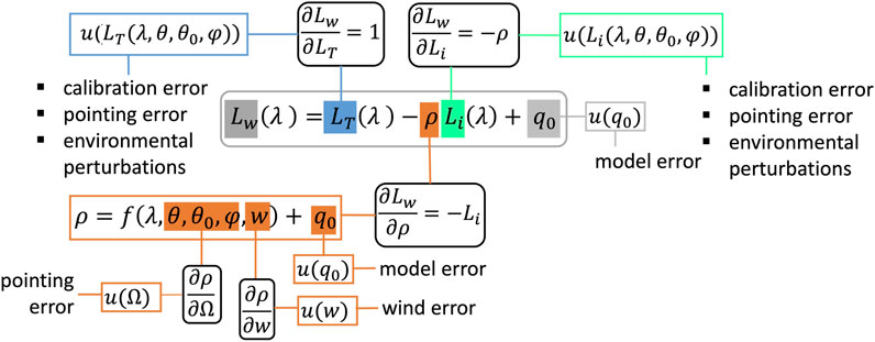
FIGURE 1. Uncertainty tree diagram for the AERONET-OC L_W measurement function (associated with Eq. 3). The measurement function is in the grey rectangle, expressing the measurand as a function of its influence quantities (or input quantities). For each input, the associated error sources are traced with various colors to their contributing factors. Rounded black rectangles indicate the sensitivity factors (expressed as partial derivatives), i.e., the extent to which an error in an input impacts the measurand. For all equations in the diagram, q₀ is a generic notation indicating a possible model error. Ω is a short notation for the geometry of observation and illumination.

The conversion from L_W to the normalized water-leaving radiance L_WN or, equivalently, to the remote sensing reflectance R_RS (L_WN and R_RS merely differ by the factor E₀, Eq. 2) is illustrated by the uncertainty tree diagram of Figure 2. For each record j, the combined standard uncertainty for L_WN, u(L_WN,j), was calculated from u(L_W,j) and the law of uncertainty propagation applied to Eq. 2, according to (also ignoring correlated terms):

$u^2\left(L_{WN,j}\right)={\left(C_{Q,j}{C}_{A,j}u\left(L_{W,j}\right)\right)}^2+{\left(L_{W,j}{u}_{\%}\left(C_{Q,j}\right)C_{Q,j}{C}_{A,j}\right)}^2+{\left(L_{W,j}{u}_{\%}\left(C_{A,j}\right)C_{A,j}{C}_{Q,j}\right)}^2(4)$

where $C_{A,j}=d_j^2\cos {\theta }_{0,j}{t}_{d,j}$, and its relative uncertainty u_%(C_A) is assumed constant for all center-wavelengths and equal to 1.5% (Zibordi et al., 2009b). This estimate encompasses several sources of error such as those due to aerosol, ozone and Rayleigh optical thickness and related optical properties (Figure 2). The relative uncertainty associated with C_Q (term correcting for bidirectional effects), u_%(C_Q,j), is calculated for each record j as in Cazzaniga and Zibordi (2023), differently when considering Chl-based or IOP-based bidirectional correction functions. Uncertainty values associated with R_RS were eventually obtained from u(L_WN) by dividing by E₀ considered as well known [in reality, this step could introduce an additional, spectrally-varying, uncertainty contribution of the order of 1%, Figure 2, Thuillier et al. (1998)]. Finally, uncertainty estimates shown in this work could slightly vary from those reported in Cazzaniga and Zibordi (2023) due to an updated AERONET-OC time-series which includes more recent data.

FIGURE 2

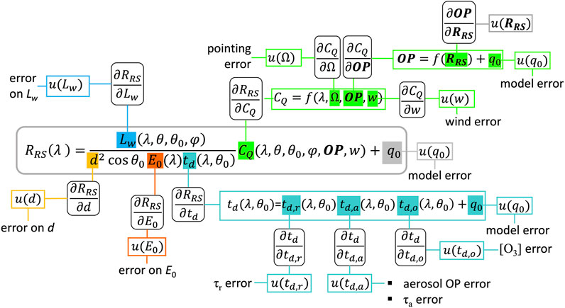
FIGURE 2. Uncertainty tree diagram for the conversion from L_W to R_RS (associated with Eq. 4). Its construction is similar to Figure 1. Bold notations indicate a spectrum of values for R_RS or for optical properties OP. t_d,r, t_d,a, and t_d,o are transmittance associated with air molecules (Rayleigh), aerosol and ozone. τ_r is the Rayleigh optical thickness (dependent on tabulated values at the standard atmospheric pressure and the actual atmospheric pressure).

2.3 Statistics of comparison

For each day of operation of PRS₀ and for each measurement, the data collected by PRS₁ were searched for the record with the closest time of acquisition, and the pair of coincident measurements was selected for comparison if the time difference was smaller than Δt. From the data set of N pairs of matched data ${(x_{0,i})}_{i=1,N}$ and ${(x_{1,i})}_{i=1,N}$ associated with PRS₀ and PRS₁, respectively, statistics of comparison were computed (Mélin and Franz, 2014; IOCCG, 2019), such as:

$\mathrm{\Delta }=\sqrt{\frac{1}{N}{\displaystyle \sum _{i=1}^N}{\left(x_{1,i}-x_{0,i}\right)}^2}(5)$

$\delta =\frac{1}{N}{\displaystyle \sum _{i=1}^N}\left(x_{1,i}-x_{0,i}\right)=\overline{x_1}-\overline{x_0}(6)$

${\mathrm{\Delta }}_c=\sqrt{\frac{1}{N}{\displaystyle \sum _{i=1}^N}{\left(x_{1,i}-x_{0,i}+\overline{x_0}-\overline{x_1}\right)}^2}=\sqrt{{\mathrm{\Delta }}^2-{\delta }^2}(7)$

where the overbar indicates an average value. Δ, the root-mean-square (RMS) difference between x₀ and x₁ (Eq. 5), can be expressed as the sum (in quadratic form) of the average difference (also called bias), δ, and the centered RMS difference Δ_c.

Acknowledging that there was no reason to consider one measurement better than the other, relative differences were quantified using their unbiased (or symmetric) form, i.e., taking the average of x₀ and x₁ as a reference (at the denominator) (e.g., Hooker and Morel, 2003; Mélin and Franz, 2014).

$|{\psi }_u{|}_m=\text{median}{\left(\frac{2|x_{1,i}-x_{0,i}|}{x_{0,i}+x_{1,i}}\right)}_{i=1,N}(8)$

${\psi }_{u,m}=\text{median}{\left(\frac{2\left(x_{1,i}-x_{0,i}\right)}{x_{0,i}+x_{1,i}}\right)}_{i=1,N}(9)$

The “median” operator was adopted to reduce the possible impact of outliers; |ψ_u|_m is the median unbiased absolute relative difference (here “absolute” refers to the use of the modulus operator | |, Eq. 8) and ψ_u,m is the median unbiased relative difference (Eq. 9).

The Pearson correlation coefficient r between coincident PRS₀ and PRS₁ measurements (R_RS or τ_a) was also computed.

2.4 Error model for collocation statistics

Going beyond simple comparison statistics, collocation analysis underpinned by an error model can provide more elaborate statistics characterizing uncertainties (Stoffelen, 1998; Toohey and Strong, 2007). Here the following error model was adopted for the records ${(x_{0,i})}_{i=1,N}$ and ${(x_{1,i})}_{i=1,N}$ associated with PRS₀ and PRS₁, respectively:

$x_{0,i}=t_i+{ϵ}_{0,i}(10)$

$x_{1,i}=\alpha +\beta t_i+{ϵ}_{1,i}(11)$

where t is a reference value and the ϵ′s are zero-mean random error terms. The term t that serves as a link between x₀ and x₁ can be related to the true value and is not impacted by non-systematic effects that are captured by ϵ. Additive and multiplicative biases, α and β, respectively, further relate x₀ and x₁. Besides systematic effects, uncertainties of x₀ and x₁ could be characterized by the standard deviation of the associated ${({ϵ}_i)}_{i=1,N}$, σ_ϵ.

This framework was adopted to investigate uncertainties of satellite values (Mélin, 2010; Mélin et al., 2016; Mélin, 2021; Mélin, 2022) with the assumption that the ϵ terms were uncorrelated with t and with each other. Considering that the simultaneous determination of R_RS by the 2 PRS systems share some elements (Figures 1, 2), this assumption is not warranted here and the framework was extended to the case where ϵ₀ and ϵ₁ are correlated with a coefficient r_ϵ. Writing the variance and covariance terms associated with x₀ and x₁ in that case leads to:

${\sigma }_0^2={\sigma }_t^2+{\sigma }_{ϵ0}^2(12)$

${\sigma }_{01}=\beta {\sigma }_t^2+r_{ϵ}{\sigma }_{ϵ0}{\sigma }_{ϵ1}(13)$

${\sigma }_1^2={\beta }^2{\sigma }_t^2+{\sigma }_{ϵ1}^2(14)$

where σ₀ and σ₁ are the standard deviation of x₀ and x₁, respectively, and σ_ϵ0 and σ_ϵ1 the standard deviation of ϵ₀ and ϵ₁, respectively.

This system can be rewritten by removing σ_t from Eqs 12, 14 using Eq. 13:

${\sigma }_0^2=\frac{{\sigma }_{01}-r_{ϵ}{\sigma }_{ϵ0}{\sigma }_{ϵ1}}{\beta }+{\sigma }_{ϵ0}^2(15)$

${\sigma }_1^2=\beta \left({\sigma }_{01}-r_{ϵ}{\sigma }_{ϵ0}{\sigma }_{ϵ1}\right)+{\sigma }_{ϵ1}^2(16)$

This system with two equations and four unknowns can be solved if the ratio σ_ϵ1/σ_ϵ0, noted η, and r_ϵ are known. This leads to a second-order polynomial with the solution:

$\beta =\frac{{\sigma }_1^2-{\eta }^2{\sigma }_0^2+\sqrt{{\left({\sigma }_1^2-{\eta }^2{\sigma }_0^2\right)}^2+4\left({\sigma }_{01}-r_{ϵ}\eta {\sigma }_0^2\right)\left({\eta }^2{\sigma }_{01}-r_{ϵ}\eta {\sigma }_1^2\right)}}{2\left({\sigma }_{01}-r_{ϵ}\eta {\sigma }_0^2\right)}(17)$

The case r_ϵ = 0 reduces β to the slope of the model II regression, and to the slope of a simple major-axis regression if additionally η = 1 (Legendre and Legendre, 1998).

The value of β finally leads to σ_ϵ0 and σ_ϵ1 that are considered as the uncertainties associated with x₀ and x₁ (excluding systematic effects).

${\sigma }_{ϵ0}^2=\frac{\beta {\sigma }_0^2-{\sigma }_{01}}{\beta -r_{ϵ}\eta }(18)$

${\sigma }_{ϵ1}^2=\frac{{\sigma }_1^2-\beta {\sigma }_{01}}{1-\beta r_{ϵ}/\eta }(19)$

3 Results

3.1 General statistics on data and uncertainties

During the common period of operations (∼5.5 years), PRS₀ produced Level 2.0 data over 1,112 days totaling 14,700 records, while data were collected by PRS₁ in 811 days (3,059 records). The difference in the number of acquisitions is mostly explained by the higher frequency of observation granted by the CE-318T system (PRS₀).

Figure 3 shows the median values for R_RS and associated median uncertainty u(R_RS) for both terms $R_{RS}^{\mathit{Chl}}$ and $R_{RS}^{\mathit{IOP}}$. R_RS values are typical of the AAOT site, representative of coastal waters with moderately turbid conditions and a peak at 490–530 nm (or secondarily at 555–560 nm) (e.g., Zibordi et al., 2021). The median spectra R_RS display a remarkable agreement, both between methods ($R_{RS}^{\mathit{Chl}}$ and $R_{RS}^{\mathit{IOP}}$) and between systems (PRS₀ and PRS₁), in the latter case when wavelengths are coincident. The spectra u(R_RS) have a broadly similar shape, with the highest values in the interval 490–560 nm, with lower values in the blue and much lower values in the red. The median spectra u(R_RS) for PRS₁ usually appear higher than for PRS₀, which is due mostly to the different amounts of data (these differences largely disappear when considering common records, see below).

FIGURE 3

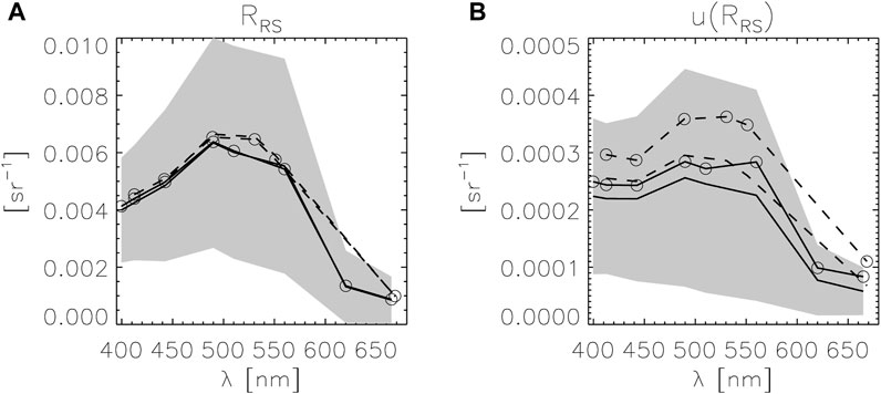
FIGURE 3. Overall average statistics: (A) Spectrum of median R_RS for PRS₀ (line) and PRS₁ (dashed line), for $R_{RS}^{\mathit{Chl}}$ (line and circle) and for $R_{RS}^{\mathit{IOP}}$ (simple line), the grey envelope representing ± the standard deviation of $R_{RS,0}^{\mathit{IOP}}$; (B) Median uncertainty u (R_RS) for PRS₀ (line) and PRS₁ (dashed line), for $u(R_{RS}^{\mathit{Chl}})$ (line and circle) and for $u(R_{RS}^{\mathit{IOP}})$ (simple line), the grey envelope representing ± the standard deviation of $u(R_{RS,0}^{\mathit{IOP}})$.

The overall median aerosol optical thickness τ_a decreases from 0.167 (standard deviation, s.d., 0.133) at 412 nm to 0.054 (s.d. 0.051) at 865 nm for PRS₀, and from 0.166 (s.d. 0.143) at 412 nm to 0.055 (s.d. 0.056) at 869 nm for PRS₁. The median Ångström exponent [computed with a log-transformed linear regression for bands between 412 and 869 nm, Ångström, (1964)] is equal to 1.55 (s.d. 0.30) and 1.52 (s.d. 0.31) for PRS₀ and PRS₁, respectively. These values are also typical for the site and representative of the continental aerosols encountered in the region (Mélin and Zibordi, 2005; Mélin et al., 2006; Clerici and Mélin, 2008).

Focusing on the uncertainties of R_RS (calculated assuming uncorrelated inputs, see Section 2.2), Figure 4 shows the distribution functions of $u(R_{RS}^{\mathit{Chl}})$ and $u(R_{RS}^{\mathit{IOP}})$ for PRS₀, (results for PRS₁ are similar with slightly higher values). Results are consistent with those given by Cazzaniga and Zibordi (2023), with median $u(R_{RS}^{\mathit{Chl}})$ and $u(R_{RS}^{\mathit{IOP}})$ in the interval 2.2–2.8 10⁻⁴ sr⁻¹ for wavelengths below 665 nm for PRS₀ (2.5–3.6 10⁻⁴ sr⁻¹ for PRS₁). For PRS₀, median values at 665 nm are 0.83 10⁻⁴ sr⁻¹ for $u(R_{RS}^{\mathit{Chl}})$ and 0.58 10⁻⁴ sr⁻¹ for $u(R_{RS}^{\mathit{IOP}})$ (1.1 and 0.68 10⁻⁴ sr⁻¹ for PRS₁ at 667 nm). The distributions for $u(R_{RS}^{\mathit{Chl}})$ and $u(R_{RS}^{\mathit{IOP}})$ are fairly similar, with the former showing a longer tail of high values. In that respect, the corresponding distributions for the relative uncertainties (Figure 5) show more pronounced differences, with $u_{\%}(R_{RS}^{\mathit{Chl}})$ extending towards larger values. Considering both PRS₀ and PRS₁, the median $u_{\%}(R_{RS}^{\mathit{IOP}})$ is in the interval 4.2%–5.4% for wavelengths below 665 nm, and increases to ∼6.2% at 665–667 nm; the median $u_{\%}(R_{RS}^{\mathit{Chl}})$ is slightly higher, in the interval 4.4%–6.4% for wavelengths below 665 nm, and 10.1%–12.1% at 665–667 nm.

FIGURE 4

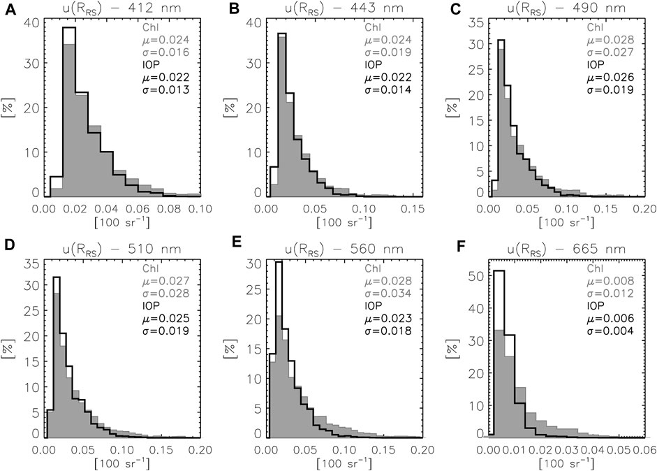
FIGURE 4. Normalized distribution functions of the uncertainties u(R_RS) for PRS₀ at (A) 412 nm, (B) 443 nm, (C) 490 nm, (D) 510 nm, (E) 560 nm and (F) 665 nm. Grey histogram and statistics are associated with $u(R_{RS}^{\mathit{Chl}})$, while black line and statistics are associated with $u(R_{RS}^{\mathit{IOP}})$. μ and σ give median and standard deviation, respectively.

FIGURE 5

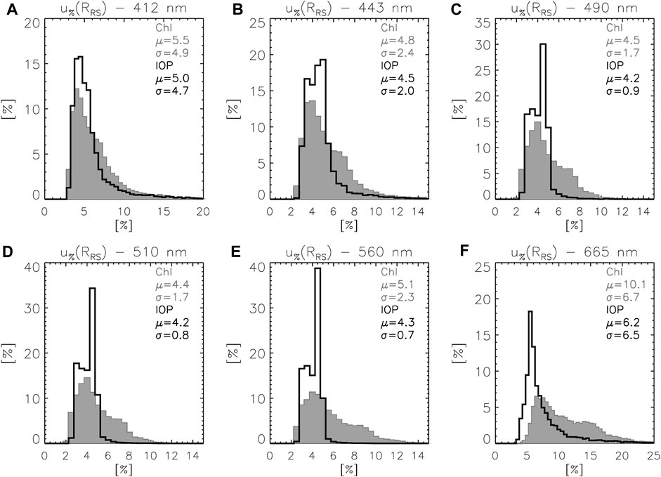
FIGURE 5. Normalized distribution functions of the relative uncertainties u_%(R_RS) for PRS₀ at (A) 412 nm, (B) 443 nm, (C) 490 nm, (D) 510 nm, (E) 560 nm and (F) 665 nm. Grey histogram and statistics are associated with $u_{\%}(R_{RS}^{\mathit{Chl}})$, while black line and statistics are associated with $u_{\%}(R_{RS}^{\mathit{IOP}})$. μ and σ give median and standard deviation, respectively.

3.2 Comparison of τ_a and R_RS data

Selecting a maximum time difference Δt of 10 min, 659 days have at least one pair of matching observations, amounting to a total of 4,449 pairs. This short time difference is associated with similar conditions of illumination, with a mean absolute difference of 0.49° for the solar zenith angle and 1.9° for the solar azimuth angle. In this matching exercise, several members of each PRS₀ triplet (up to 3) can be associated with the same PRS₁ record. Enforcing the occurrence of the PRS₁ data in one matching pair only would reduce the number of matching pairs by half: it would exclude some members of the associated PRS₀ triplet and ultimately a considerable number of valid observations in an arbitrary way. The option adopted here is to consider all PRS₀ data as valid independent observations to be compared to PRS₁ observations. Importantly, besides a lower number of match-ups, results are not affected by this choice.

The comparison between τ_a from PRS₀ and PRS₁ shows a remarkable agreement with a determination coefficient r² decreasing from 0.994 at 412 nm to 0.977 at 865 nm, maximum RMS differences Δ of ∼0.01 in the spectral range 412–560 nm, and median unbiased absolute relative differences |ψ_u|_m lower than 5% (6.5% at 865 nm) (see Table 1 and Figure 6). There are very few outliers that might be associated with cases of rapid changes in the atmosphere. For instance on 25 February 2020 (the case associated with the highest τ_a in Figure 6), PRS₀ detected three values of τ_a (412) in a hour, 1.26, 1.25 and 1.67, while PRS₁ recorded only one value (1.38) 6 min before the third PRS₀ record.

TABLE 1

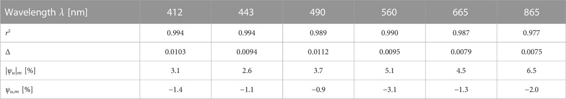
TABLE 1. Comparison statistics for τ_a with determination coefficient r², RMS difference Δ, median unbiased absolute relative difference |ψ_u|_m and median unbiased relative difference ψ_u,m. Positive values indicate that τ_a from PRS₁ is higher than from PRS₀.

FIGURE 6

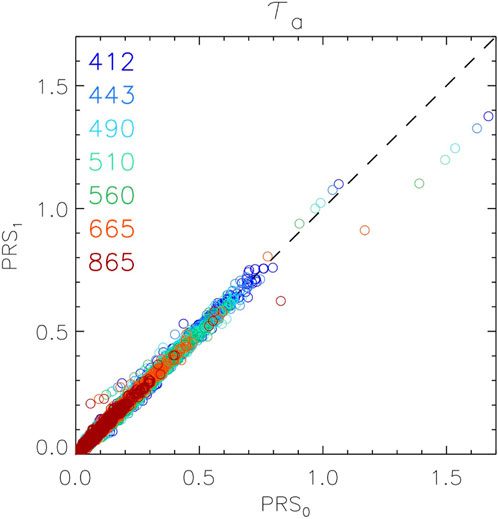
FIGURE 6. Scatter plot of τ_a between PRS₀ and PRS₁ for the indicated wavelengths. Statistics of comparison are given in Table 1.

The R_RS data from the two systems also agree very well with very few outliers (Figure 7) in agreement with preliminary results found in Zibordi et al. (2021). This is true for both $R_{RS}^{\mathit{Chl}}$ and $R_{RS}^{\mathit{IOP}}$, with Δ of the order of 3 10⁻⁴ sr⁻¹ (except ∼1.66 10⁻⁴ sr⁻¹ at 665 nm), |ψ_u|_m of 2%–3% (except 5.8% at 665 nm), median unbiased relative differences ψ_u,m around or below 1% (except 2.5% at 665 nm) and r² in the range 0.967–0.994 (Table 2).

FIGURE 7

FIGURE 7. Scatter plots comparing (A) $R_{RS}^{\mathit{Chl}}$ and (B) $R_{RS}^{\mathit{IOP}}$ from PRS₀ and PRS₁ for the indicated wavelengths. Statistics of comparison are given in Table 2.

TABLE 2

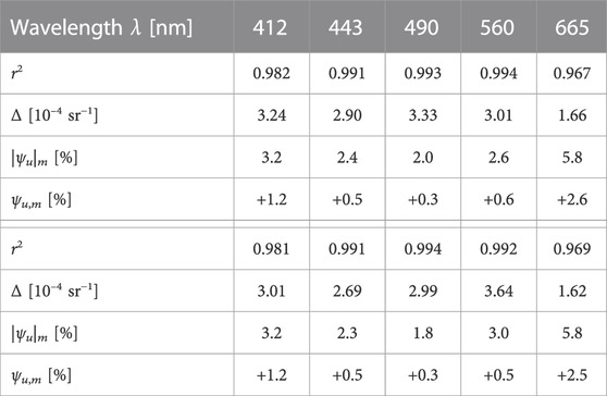
TABLE 2. Comparison statistics for $R_{RS}^{\mathit{Chl}}$ (upper part) and $R_{RS}^{\mathit{IOP}}$ (lower part) with determination coefficient r², RMS difference Δ, median unbiased absolute relative difference |ψ_u|_m and median unbiased relative difference ψ_u,m. Positive values indicate that R_RS from PRS₁ is higher than from PRS₀.

3.3 Uncertainty estimates versus comparison statistics

Considering the similar conditions of observations associated with the matched data and the common method to derive uncertainty estimates, u(R_RS) from PRS₀ and PRS₁ are expected to be close, which is indeed verified by Figure 8. For both $u(R_{RS}^{\mathit{Chl}})$ and $u(R_{RS}^{\mathit{IOP}})$, r² between the two distributions is ∼0.98. For $u(R_{RS}^{\mathit{Chl}})$, Δ is ∼0.2 10⁻⁴ sr⁻¹, except at 560 nm where it is 0.6 10⁻⁴ sr⁻¹. In the case of the green band, there are more outliers and an overestimate of the uncertainty from PRS₀ with respect to $u(R_{RS}^{\mathit{Chl}})$ from PRS₁. This can not be easily explained by differences in center wavelengths, as R_RS would tend to decrease (and likely its related uncertainty) from 551–555 nm (typical of PRS₁) to 560 nm (associated with PRS₀). Except few outliers, the agreement is slightly better for $u(R_{RS}^{\mathit{IOP}})$ (Figure 8B) with Δ in the interval 0.15–0.25 10⁻⁴ sr⁻¹ between 412 and 560 nm (and 0.08 10⁻⁴ sr⁻¹ at 665 nm); in agreement with Figure 4, there are also less $u(R_{RS}^{\mathit{IOP}})$ values in the upper range (and none above 1.4 10⁻³ sr⁻¹).

FIGURE 8

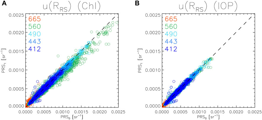
FIGURE 8. Scatter plots comparing (A) $u(R_{RS}^{\mathit{Chl}})$ and (B) $u(R_{RS}^{\mathit{IOP}})$ from PRS₀ and PRS₁ for the indicated wavelengths.

The uncertainty estimates should now be related to the differences between coincident records of R_RS from PRS₀ and PRS₁ documented in the previous Section 3.2. The uncertainty associated with the difference R_RS,1 − R_RS,0 can be expressed with (Mélin, 2021):

$u^2\left(R_{RS,1}-R_{RS,0}\right)=u^2\left(R_{RS,0}\right)+u^2\left(R_{RS,1}\right)-2r\left(e\left(R_{RS,0}\right),e\left(R_{RS,1}\right)\right)u\left(R_{RS,0}\right)u\left(R_{RS,1}\right)(20)$

where r(e(R_RS,0), e(R_RS,0)) is the correlation between the errors associated with R_RS,0 and R_RS,1. If this correlation is null in Eq. 20, the uncertainty associated with the difference is the sum of the uncertainties (in quadratic form) [e.g., Immler et al. (2010)]. The following inequality may then be introduced (Kacker et al., 2010; Mélin, 2021):

$|R_{RS,1}-R_{RS,0}|<k\sqrt{u^2\left(R_{RS,0}\right)+u^2\left(R_{RS,1}\right)-2r\left(e\left(R_{RS,0}\right),e\left(R_{RS,1}\right)\right)u\left(R_{RS,0}\right)u\left(R_{RS,1}\right)}(21)$

where k is the so-called coverage factor. With a normal hypothesis, this inequality would be true in 68% of cases with a coverage factor k = 1. Strictly speaking, this reasoning is valid for a hypothetical situation where multiple measurements are repeated in identical conditions; it was here extended to the current match-up data set where R_RS (and their uncertainties) are associated with varying conditions experienced during years of operations. No estimate is readily available to quantify the term associated with error correlation (see further on for discussion on this issue) and four cases were considered (with the correlation coefficient assumed constant across the data set): no correlation, low correlation (0.2), moderate correlation (0.5) and high correlation (0.7). The percentage κ of records where Eq. 21 is true appears much higher than 68% for $R_{RS}^{\mathit{Chl}}$ (Table 3); only in the worst case scenario (r = 0.7) does κ become slightly lower than 68% at 412 and 665 nm. For $R_{RS}^{\mathit{IOP}}$ between 412 and 490 nm, κ is only slightly lower than for $R_{RS}^{\mathit{Chl}}$ (and mostly well above 68% except at 412 nm for r = 0.7) but is noticeably lower at 560 and 665 nm, and lower than 68% for an error correlation above 0.5. Average differences between PRS₀ and PRS₁ are similar for $R_{RS}^{\mathit{Chl}}$ and $R_{RS}^{\mathit{IOP}}$ (actually higher in the latter case at 560 nm, Table 2), while uncertainty estimates tend to be lower for $R_{RS}^{\mathit{IOP}}$ than for $R_{RS}^{\mathit{Chl}}$ (Figures 4, 5), which explains why Eq. 21 is less often verified for $R_{RS}^{\mathit{IOP}}$, and ultimately the degraded results obtained for κ associated with $R_{RS}^{\mathit{IOP}}$.

TABLE 3

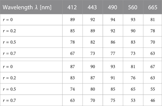
TABLE 3. Fractions κ (given in %) of records where Eq. 21 is verified for $R_{RS}^{\mathit{Chl}}$ (upper part) and $R_{RS}^{\mathit{IOP}}$ (lower part) and for the four cases of error correlation.

The previous analysis was conducted with statistics compiled over the whole data set; taking advantage of the amount of data available, it can be completed by a more detailed analysis along the range of uncertainties. The set of uncertainties u(R_RS) was split into 20 bins of equal sample size for which the average value was computed. Then, the centered RMS difference Δ_c (Eq. 7) and average difference δ (Eq. 6) between R_RS from PRS₀ and PRS₁ were computed using the records associated with each bin.

Results for $R_{RS}^{\mathit{Chl}}$ and $R_{RS}^{\mathit{IOP}}$ are shown for representative wavelengths in the uncertainty “cone diagrams” of Figures 9, 10, respectively. For each bin, the vertical bar represents ±Δ_c (that is the standard deviation of R_RS,1 − R_RS,0) while the circle shows δ (the dotted lines being the ±1:1 lines). This type of graphs is more readily used to verify uncertainty estimates when a data set y (typically satellite retrievals) is compared with reference data x (typically field data) (e.g., Ghent et al., 2019). If the error associated with x is negligible, Δ_c is the standard deviation of the errors associated with y and the extremities of the vertical bars should follow the dotted lines (with the assumption that the errors of x and y are not correlated). The dotted uncertainty lines are not extended to 0: in the case of a comparison with reference data, the cone is extended on the lower range by horizontal lines that represent the uncertainty associated with these reference data, considered as the minimum possible value (in the current case the uncertainty lines are only displayed for the available range). Vertical bars exceeding the conic envelope of the dotted lines would indicate that the uncertainty values are underestimated (i.e., that the actual uncertainties would be higher), while vertical bars well contained within the dotted envelope would suggest the opposite. In the current study, neither PRS₀ nor PRS₁ can be taken as a reference value, which means that the comparison between estimated uncertainties and Δ_c remains imperfect. It can just be noted that if the true value of R_RS happened to be always in the interval [R_RS,0; R_RS,1], then Δ_c would be larger than the uncertainty.

FIGURE 9

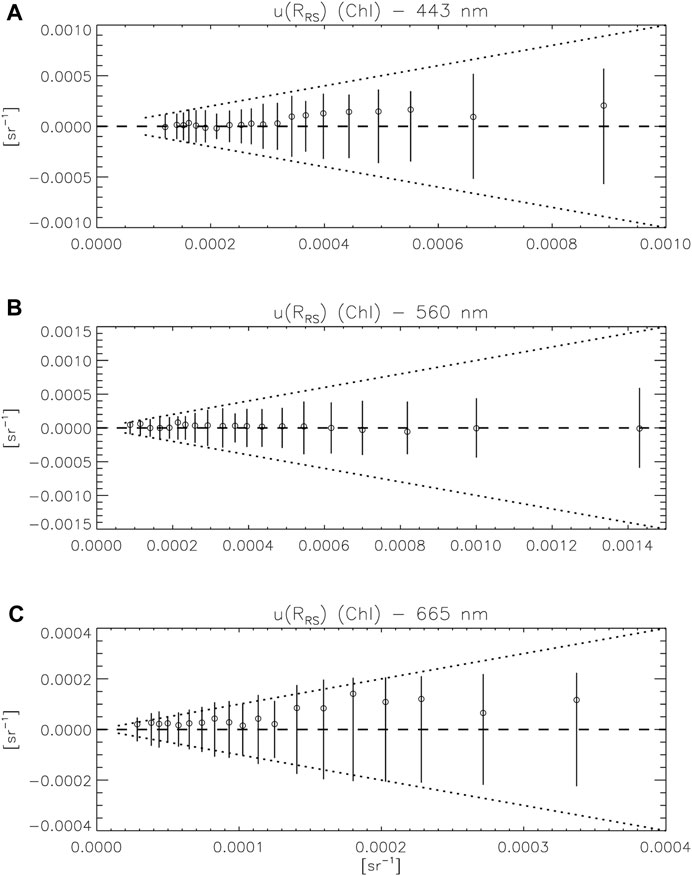
FIGURE 9. Comparison between uncertainty estimates $u(R_{RS}^{\mathit{Chl}})$ and comparison statistics through an uncertainty cone diagram at (A) 443 nm, (B) 560 and (C) 665 nm. The vertical bars represented ±Δ_c computed between $R_{RS,0}^{\mathit{Chl}}$ and $R_{RS,1}^{\mathit{Chl}}$ for each bin of increasing uncertainty $u(R_{RS}^{\mathit{Chl}})$. Circles are the associated average difference between $R_{RS,0}^{\mathit{Chl}}$ and $R_{RS,1}^{\mathit{Chl}}$. Dotted lines are ±1:1 lines.

FIGURE 10

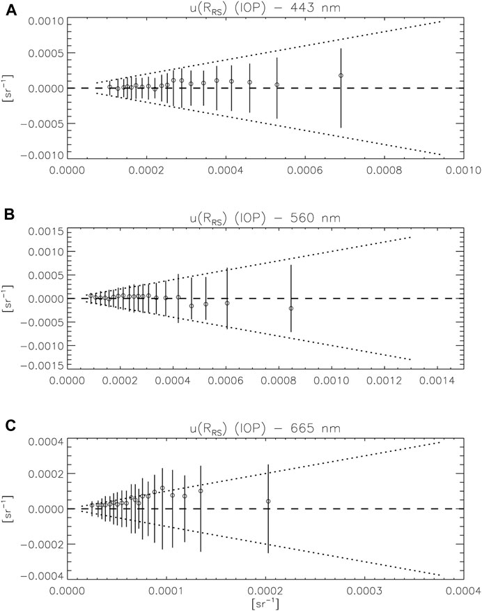
FIGURE 10. Comparison between uncertainty estimates $u(R_{RS}^{\mathit{IOP}})$ and comparison statistics through an uncertainty cone diagram at (A) 443 nm, (B) 560 and (C) 665 nm. The vertical bars represented ±Δ_c computed between $R_{RS,0}^{\mathit{IOP}}$ and $R_{RS,1}^{\mathit{IOP}}$ for each bin of increasing uncertainty u$(R_{RS}^{\mathit{IOP}})$. Circles are the associated average difference between $R_{RS,0}^{\mathit{IOP}}$ and $R_{RS,1}^{\mathit{IOP}}$. Dotted lines are ±1:1 lines.

At almost all wavelengths and across the range of reported uncertainties, the average differences δ between R_RS,0 and R_RS,1 is well below the uncertainty (circles in the dotted cone in Figures 9, 10), the exception being the case of $R_{RS}^{\mathit{IOP}}$ at 665 nm where δ is close to $u(R_{RS}^{\mathit{IOP}})$ (Figure 10C). For $R_{RS}^{\mathit{Chl}}$ between 412 and 560 nm, the extremities of the vertical bars ±Δ_c tend to follow the uncertainty estimates (the dotted lines) in the low range of values; in the higher range of uncertainty values, ±Δ_c remains further away from the conic envelop (for instance, at 560 nm Δ_c tends to remain stable above uncertainties of 3 10⁻⁴ sr⁻¹, Figure 9B), suggesting that uncertainty values could actually be too high. The same behavior is seen at 665 nm but the extremities of ±Δ_c follow the uncertainty estimates for almost the entire uncertainty range (Figure 9C). For $R_{RS}^{\mathit{IOP}}$ (Figure 10), the extremities of ±Δ_c closely follow the cone lines (or are included within the cone) across the range of reported uncertainties from 412 to 560 nm, while at 665 nm, they exceed the uncertainty estimates, suggesting that reported uncertainties may be too low. This is of course coherent with the relatively low values obtained for κ in that case (Table 3). Again, the interpretation that can be given about the positions of the vertical bars ±Δ_c within (or beyond) the uncertainty cone implicitly assumes that the error correlation between the PRS₀ and PRS₁ records is negligible. If this is not the case, conclusions drawn from the cone diagrams are too favorable to an extent dependent on the error correlation (Section 3.6). The cone diagram analysis is still valuable as complementary to the analysis conducted with all data (Table 3) as it looks at the behavior of statistics across the range of uncertainties.

3.4 Uncertainty estimates versus collocation statistics for τ_a

The collocation approach was first applied to the aerosol optical thickness data τ_a. Considering the agreement of the τ_a data from PRS₀ and PRS₁ (Figure 6), the choice of η = 1 (ratio of the σ_ϵ’s) appears justified. A value for the error correlation is also required and four cases are again considered with r_ϵ equal to 0, 0.2, 0.5 and 0.7. For the case of r_ϵ = 0, the value of β varies between 0.996 and 1.011 (at 865 nm) (Table 4), values that are barely affected by the choice of r_ϵ. σ_ϵ tends to decrease with wavelength, e.g., from 0.0072 at 412 nm to 0.0053 at 865 nm for r_ϵ = 0. Contrary to β, σ_ϵ increases with r_ϵ (following Eqs. 18, 19), from 0.0072 for r_ϵ = 0 to 0.0131 for r_ϵ = 0.7 at 412 nm, or from 0.0053 to 0.0096 at 865 nm. These results are mostly lower than reported uncertainties (Eck et al., 1999; Schmid et al., 1999) of 0.01–0.015 (in the interval 412–865 nm, decreasing with wavelength) but are very close in the case of r_ϵ = 0.7. Similar inputs in environmental variables used in τ_a retrieval, such as atmospheric pressure for the determination of the Rayleigh optical depth or ozone concentration and properties, would result in an error correlation for two instruments functioning simultaneously, whereas effects such as instrument noise would not. While determining the relative weights of correlated and uncorrelated effects in τ_a retrievals is out of the scope of this work, it can be said that, unless the contribution to the uncertainty budget from environmental variables is dominant, leading to the upper value of the error correlation, σ_ϵ is found somewhat lower than reported uncertainty values; but it is also stressed that σ_ϵ does not contain contributions from systematic effects (these would be captured by α and β in Eqs. 10, 11), which can be significant (Giles et al., 2019). For completeness, it is noted that the median difference between τ_a from PRS₀ and PRS₁ varies (in modulus) between 0.0010 and 0.0033. Overall, collocation statistics appear consistent with reported uncertainty values for τ_a.

TABLE 4

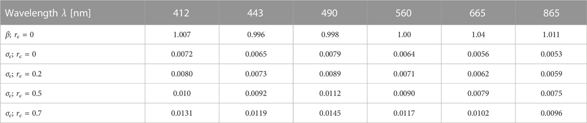
TABLE 4. Collocations statistics: regression slope β for r_ϵ = 0, and σ_ϵ for τ_a for four cases of error correlation r_ϵ.

3.5 Uncertainty estimates versus collocation statistics for R_RS

A similar analysis was conducted with R_RS with results reported in Table 5 for the same four cases of error correlation r_ϵ (this time relative to R_RS), again under the assumption of η = 1 considering the agreement in R_RS illustrated in Figures 7, 8. The value of β is only given for r_ϵ = 0 since it hardly varies with r_ϵ (with values very close to 1). As for τ_a and according to Eqs 18, 19, σ_ϵ increases with r_ϵ for both $R_{RS}^{\mathit{Chl}}$ and $R_{RS}^{\mathit{IOP}}$, typically from ∼2 to ∼3 10⁻⁴ sr⁻¹ (for wavelengths between 412 and 560 nm) when r_ϵ increases from 0 to 0.5. σ_ϵ increases again significantly if r_ϵ is increased from 0.5 to 0.7 (reaching ∼4 10⁻⁴ sr⁻¹).

TABLE 5

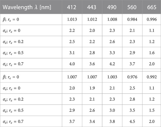
TABLE 5. Collocations statistics β for r_ϵ = 0, and σ_ϵ (in 10^–4 sr⁻¹) for $R_{RS}^{\mathit{Chl}}$ (upper part) and $R_{RS}^{\mathit{IOP}}$ (lower part) and for four cases of error correlation r_ϵ.

Values of σ_ϵ can eventually be compared with other statistics presented in the previous sections, the median uncertainty estimate u(R_RS) (for both PRS₀ and PRS₁, computed with the common records of the match-up data set) and the RMS difference between R_RS from PRS₀ and PRS₁ in its centered form Δ_c since σ_ϵ does not include systematic contributions (the average difference δ is also illustrated for completeness and comparison with non-systematic terms). In agreement with Section 2.1 and Figure 4, the median $u(R_{RS}^{\mathit{IOP}})$ is lower than $u(R_{RS}^{\mathit{Chl}})$ (compare Figures 11A, B), while the related Δ_c are comparable, except at 560 nm, where values are higher for $R_{RS}^{\mathit{IOP}}$. As a result, for $R_{RS}^{\mathit{Chl}}$, u(R_RS) is similar or higher than Δ_c except at 665 nm where u(R_RS) becomes lower (Figure 11A), while for $R_{RS}^{\mathit{IOP}}$, u(R_RS) is clearly lower than Δ_c at 560 and 665 nm (Figure 11B). For low values of r_ϵ (0 and 0.2), σ_ϵ associated with $R_{RS}^{\mathit{Chl}}$ is lower than u(R_RS) except at 665 nm, while for $R_{RS}^{\mathit{IOP}}$, σ_ϵ is lower than u(R_RS) for 412–490 nm, similar for 560 nm and higher for 665 nm. Interestingly, σ_ϵ is very close to Δ_c if r_ϵ = 0.5. For the case of highest correlation (0.7), σ_ϵ is to a varying extent higher than both Δ_c and u(R_RS).

FIGURE 11

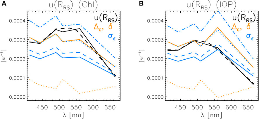
FIGURE 11. Spectra of the median reported uncertainty u (R_RS) (black line for PRS₀ and black dashed line for PRS₁) computed for coincident measurements, spectra of centered RMS differences Δ_c (orange line) and average differences δ (orange dotted line), and spectra of σ_ϵ for r_ϵ = 0 (blue line), 0.2 (blue dashed line), 0.5 (blue dotted line) and 0.7 (blue dashed-dotted line). Results are given for (A) $R_{RS}^{\mathit{Chl}}$ and (B) $R_{RS}^{\mathit{IOP}}$.

The relation between Δ_c and σ_ϵ can be further discussed by relating Δ_c with terms of variance and covariance of ${(x_{0,i})}_{i=1,N}$ and ${(x_{1,i})}_{i=1,N}$ in Eqs 12–14, starting from:

${\mathrm{\Delta }}_c^2={\sigma }_0^2+{\sigma }_1^2-2{\sigma }_{01}(22)$

Eq. 22 then leads to:

${\mathrm{\Delta }}_c^2={\left(\beta -1\right)}^2{\sigma }_0^2+\left(\beta \left(2-\beta \right)+{\eta }^2-2r_{ϵ}\eta \right){\sigma }_{ϵ0}^2(23)$

In the case where η ∼1, if β → 1, then ${\mathrm{\Delta }}_c^2\to 2(1-r_{ϵ}){\sigma }_{ϵ}^2$, that is equal to ${\sigma }_{ϵ}^2$ if r_ϵ = 0.5 (if η is different from 1, the same phenomenon happens at a different value of r_ϵ), a behavior noted in Figure 11. This is actually an important result, predicting that the centered RMS difference between data collected by two systems is a conservative estimate of the uncertainty associated with these data (excluding systematic contributions) if these uncertainties can be assumed similar (η around 1) with errors moderately correlated (typically lower than 0.5) and if the slope of the major-axis regression between the two data sets is close to 1. If the errors can be assumed uncorrelated, then Δ_c is actually twice the uncertainty σ_ϵ. Values of η different from 1 would just vary the relative values of Δ_c and σ_ϵ, while a departure of β from 1 would make these results more dependent on the considered data set (through the first right-hand side term in Eq. 23 proportional to σ₀).

3.6 Error correlation associated with matched R_RS observations

The issue of the correlation of the errors associated with the matched R_RS data from PRS₀ and PRS₁ has appeared in the previous analyses, when comparing reported uncertainty estimates and comparison statistics (Section 3.3; Eq. 21) and when computing collocation statistics (Section 3.5). Admittedly, additional analyses would be required to quantify the level of correlation between errors affecting simultaneous measurements of R_RS. It could change with observation conditions and would certainly vary with wavelength as the weights of different contributing factors in the uncertainty budget varies spectrally (Cazzaniga and Zibordi, 2023). The following discussion attempts to provide an approximate range of values for the error correlation between L_WN (or R_RS) data from PRS₀ and PRS₁ by defining informed guesses on the error correlation associated with these contributing factors. Cazzaniga and Zibordi (2023) detail five major contributions to the overall uncertainty budget for L_WN, the uncertainties due to: i) the calibration of the sensor, u_cal, ii) the sea surface reflectance factor ρ, u_ρ, iii) the normalization term for downwelling irradiance C_A = 1/(d²μ₀t_d) (Eq. 2), $u_{C_A}$, iv) the correction for bi-directional effects C_Q (Eq. 2), $u_{C_Q}$, and v) the environmental variability, u_env (note that these terms represent uncertainty contributions to the overall uncertainty and not uncertainties of the single quantities; e.g., u_ρ is not the uncertainty u(ρ) associated with ρ but the part of the total uncertainty on R_RS that ultimately depends on ρ). For each contribution, a triplet of correlation values will be proposed [low, medium, high].

Starting with the measurement function of L_W (Figure 1), evaluating the correlation of errors due to the calibration of the instruments would require assumptions on the behavior of specific calibration lamps or plaques and on the aging of the sensors, while instrument noise that could additionally affect L_T and L_i would not introduce correlated errors. As a guess for the associated error correlation r_cal, the triplet [0, 0.1, 0.3] is proposed. Environmental perturbations may affect the terms of the measurement function L_T, L_i and ρ in a similar way for the two systems but quantifying this relationship is not straightforward and only an arbitrary choice for the associated error correlation r_env is selected here, [0, 0.1, 0.3]. The case of ρ can be further discussed, particularly with respect to wind (input to the expression of ρ, Figure 1). In the processing of AERONET-OC data, wind speed is provided by re-analysis products of coarse temporal and spatial resolutions and would have virtually the same value for two measurements collected at short time intervals. If the local wind can be assumed constant for the matched measurements (i.e., in a time interval shorter than 10 min), then the error associated with the use of the re-analysis product will be identical for the two measurements, suggesting a high error correlation affecting ρ for PRS₀ and PRS₁. However, parameterizing the state of the air-sea interface at a precise moment as a function of wind speed is a simplification (represented by the term of model error q₀ in Figure 1). The two instruments are looking at virtually the same small spot on the sea surface (with a full-angle field of view of $\sim 1.2°$, Holben et al., 1998, the footprint is similar to the distance between the instruments on the supporting platform), but their acquisitions can be minutes apart with variations in surface orientation impacting the actual ρ value (D’Alimonte et al., 2021) in an uncorrelated way. Ultimately, progress on that issue could be achieved by a realistic description of the sea surface at an appropriate time frequency coupled with radiative transfer modelling. Considering these elements, for the purpose of that discussion, a moderately high level of correlation r_ρ can be selected for the errors associated with ρ, [0.1, 0.3, 0.5].

Error correlations may be more easily identified in relation to the conversion from L_W to L_WN (or R_RS) (Figure 2), introduced by quantities depending on common environmental variables such as the transmittance t_d or C_Q (as well as by E₀). The modeling of the term C_Q contributes significantly to the overall uncertainty budget to an extent that varies with wavelength and water type (Talone et al., 2018; Cazzaniga and Zibordi, 2023). Considering that R_RS provided by the two systems are very close (Figure 7), the derived IOPs and Chl used to calculate C_Q will also be very similar with correlated errors with respect to the actual IOPs and Chl (errors that would depend on the bio-optical model and on R_RS). In addition, C_Q models representing the correction for bidirectional effects as a function of IOPs or Chl are imperfect [e.g., Gleason et al. (2012); Talone et al. (2018)], which is again represented by the term q₀ associated with C_Q in Figure 2; considering that the same C_Q model was adopted when comparing data from PRS₀ and PRS₁, error correlations $r_{C_Q}$ associated with C_Q can be assumed fairly high, [0.5, 0.7, 0.9]. A similar discussion could be undertaken with t_d that depends on atmospheric variables (e.g., τ_a, ozone, surface pressure) that are very close for matched R_RS observations, while the model for computing t_d is identical for both systems. Thus, the triplet of $r_{C_A}$ values associated with C_A is also taken as [0.5, 0.7, 0.9].

For each system PRS_j (j = 0 or 1), the error ϵ_j of a given measurement can be written as the sum of errors associated with the contributions discussed above:

${ϵ}_j={ϵ}_{\mathit{cal,j}}+{ϵ}_{\rho ,j}+{ϵ}_{C_Q,j}+{ϵ}_{C_A,j}+{ϵ}_{\mathit{env,j}}(24)$

As said for the uncertainty contributions, it is stressed that the terms of Eq. 24 are representing error contributions to the final value of R_RS errors and not errors of the single quantities (e.g., ϵ_ρ is not the error on ρ but the error on R_RS that ultimately depends on an error on ρ). Assuming that the errors from different contributions are uncorrelated between PRS₀ and PRS₁ (e.g., that the errors due to environmental variability for PRS₀ are uncorrelated with errors due to C_Q for PRS₁), a calculation of the covariance ${\sigma }_{{ϵ}_0{ϵ}_1}$ between ϵ₀ and ϵ₁ gives:

${\sigma }_{{ϵ}_0{ϵ}_1}^2={\sigma }_{{ϵ}_0{ϵ}_1,cal}^2+{\sigma }_{{ϵ}_0{ϵ}_1,\rho }^2+{\sigma }_{{ϵ}_0{ϵ}_1,C_Q}^2+{\sigma }_{{ϵ}_0{ϵ}_1,C_A}^2+{\sigma }_{{ϵ}_0{ϵ}_1,env}^2(25)$

where, e.g., ${\sigma }_{{ϵ}_0{ϵ}_1,cal}$ is the covariance of ϵ_cal,j and ϵ_cal,j. Considering that a covariance between two terms is the product of their variance and their correlation, Eq. 25 can be rewritten as:

$r=\frac{1}{u_0{u}_1}[r_{\mathit{cal}}{u}_{0,cal}{u}_{1,cal}+r_{\rho }{u}_{0,\rho }{u}_{1,\rho }+r_{C_Q}{u}_{0,C_Q}{u}_{1,C_Q}+r_{C_A}{u}_{0,C_A}{u}_{1,C_A}+r_{\mathit{env}}{u}_{0,env}{u}_{1,env}](26)$

where u₀ and u₁ are the combined standard uncertainties for PRS₀ and PRS₁ data while the u₀ and u₁ terms on the right-hand side are associated with the contributions indicated in subscript (Cazzaniga and Zibordi, 2023).

Eq. 26 is applied for the three scenarios (low, medium and high values of the triplets) to calculate an informed guess of the error correlation associated with R_RS from PRS₀ and PRS₁ (Figure 12). With the various cases considered, the resulting error correlation could take values in the broad interval 0.2–0.8 with the medium case in the interval of approximately 0.4–0.6. By assuming error correlation coefficients spectrally constant for each type of contribution, the overall correlation is seen to increase from the blue to 560 nm, which can be related to the larger weight of $u_{C_Q}$ in the uncertainty budget at that wavelength (Cazzaniga and Zibordi, 2023); it then decreases in the red, where environmental variability and ρ have a larger relative contribution with respect to the other bands. It is stressed that this spectral shape would be affected if the error correlation associated with specific contributions had a spectral dependence.

FIGURE 12

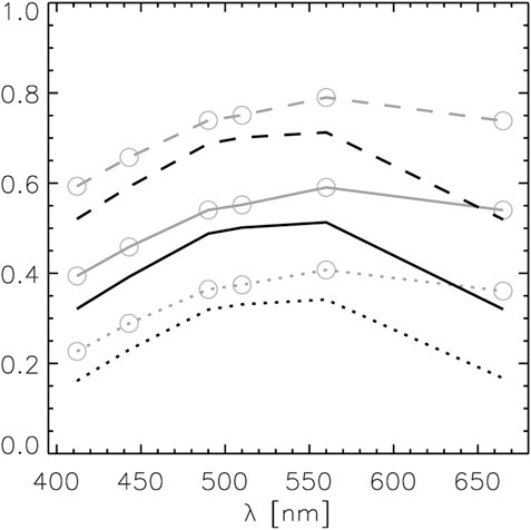
FIGURE 12. Spectra of the error correlation coefficient obtained with Eq. 26 associated with $R_{RS}^{\mathit{Chl}}$ (grey line and circles) and $R_{RS}^{\mathit{IOP}}$ (black lines) from PRS₀ and PRS₁ for the cases of low (dotted lines), medium and high (dashed lines) correlations. For the low case, [r_cal, r_ρ, $r_{C_Q}$, $r_{C_A}$, r_env], is equal to [0, 0.1, 0.5, 0.5, 0], for the medium case [0.1, 0.3, 0.7, 0.7, 0.1] and for the high case [0.3, 0.5, 0.9, 0.9, 0.3].

Looking back at Figure 11A, $u(R_{RS}^{\mathit{Chl}})$ and σ_ϵ (obtained from collocation statistics) agree well for a correlation coefficient r_ϵ of 0.5 at 412 and 443 nm, ∼0.6 at 490–560 nm, and 0–0.2 at 665 nm. In the case of $R_{RS}^{\mathit{IOP}}$ (Figure 11B), $u(R_{RS}^{\mathit{IOP}})$ and σ_ϵ agree for r_ϵ between 0.2 and 0.5 at 412–443 nm, 0.5 at 490–510 nm, and 0–0.2 at 560 nm. At 665 nm, the fact that $u(R_{RS}^{\mathit{IOP}})$ is lower than σ_ϵ obtained with r_ϵ = 0 would again suggest that it might be too low. The correlation analysis performed in this section (Figure 12) aimed at giving some sensitivity on the level of error correlation that could characterize the two systems PRS₀ and PRS₁, and the collocation statistics allowed some degree of cross-checking; this being said, a more detailed investigation would be required for more definite conclusions on this issue.

4 Conclusion

This study has taken advantage of a large body of radiometric data collected simultaneously by two instruments to assess uncertainty estimates reported for R_RS (and secondarily τ_a). The first objective was to verify these uncertainty estimates for the specific case of the AERONET-OC data collected at AAOT. τ_a and R_RS collected by the two systems appear very close (Figures 6, 7; Tables 1 and 2) and measurements generally agree within their stated uncertainties (Section 3.3), i.e., they are metrologically compatible (Kacker et al., 2010). Actually the analysis comparing uncertainty estimates u(R_RS) with comparison statistics suggested that u(R_RS) could be slightly too high in some cases (but too low for $u(R_{RS}^{\mathit{IOP}})$ at 665 nm and even at 560 nm if the error correlation between measurements of the two systems exceeds 0.5, see Table 3). However in the absence of solid estimates of error correlations linking the two systems, no definite conclusions can be stated in that respect. Uncertainty estimates also appeared compatible with uncertainty values σ_ϵ obtained using a collocation approach (again making space for undefined error correlations). Based on these considerations, even though the R_RS uncertainty budget could be further refined, the uncertainty values reported for AAOT by Cazzaniga and Zibordi (2023) generally appear trustworthy (with some exceptions where they could be too low, and for error correlation coefficients deemed realistic, i.e., not exceeding 0.7, see Section 3.6). This lends confidence to the general approach developed to calculate the AERONET-OC uncertainties, and indirectly to the resulting uncertainties associated with other sites (Cazzaniga and Zibordi, 2023, propose uncertainty estimates that are site-specific). This warrants the status of these data as reference measurements and fully supports their use for the validation of satellite data (e.g., Zibordi et al., 2022b; Mélin, 2022) and the determination of their uncertainties (Mélin, 2021).

The second objective was more methodological, aiming at applying a metrology-sound protocol to verify uncertainty estimates using simultaneous measurements, while identifying related challenges and limitations. The construction of uncertainty tree diagrams (Mittaz et al., 2019) appears very valuable for a comprehensive view of all error sources affecting a measurement system. Strictly speaking, the measuring system under study here is one quantifying the difference between R_RS observed by two instruments (i.e., R_RS,1 − R_RS,0) but for ease of illustration, uncertainty tree diagrams were given for an individual PRS system (Figures 1, 2). Uncertainty cone diagrams (Figures 9, 10) provided a mean to compare uncertainty estimates u(R_RS) with comparison statistics across their range of values. Collocation statistics also proved valuable by providing an independent method of verification. These methods could be applied to other cases where a sufficient number of coincident measurements from different systems are available, starting with the AAOT site that is regularly hosting other instruments (Vansteenwegen et al., 2019; Tilstone et al., 2020; Brando and Vilas, 2023).

The collocation framework used in previous comparison analyses (e.g., Mélin, 2021; Mélin, 2022) was here extended to cases allowing correlation between errors associated with non-systematic effects (leading to a revised expression for the slope of the model II regression, Eq. 17). This approach is powerful to verify uncertainty estimates but has also limitations. To be solved, the system of Eqs 15, 16 requires assumptions on the ratio η of uncertainties σ_ϵ and the error correlation r_ϵ. The first assumption (on the value of η) is not a major limitation as long as the σ_ϵ can be assumed comparable since the results are not strongly dependent on η (for instance η = 1.21 would multiply σ_ϵ,1 by 1.1 and σ_ϵ,0 by 0.91). As shown by Figure 11, the choice of r_ϵ has a stronger impact on σ_ϵ, and its actual value should be better characterized as acknowledged in Section 3.6. Another limitation of the collocation approach is that it provides only one general value for the whole data set (even though the current data set is actually large enough to permit computing collocation statistics on subsets of increasing R_RS) and therefore allows only the verification of average statistics of the reported uncertainties u(R_RS).

The collocation analysis has also led to a practical result, i.e., that the centered root-mean-square difference Δ_c between data collected by two systems can directly serve to quantify the uncertainty associated with these data (excluding systematic contributions); this is valid if these data show a good agreement (expressed by a slope of method II regression close to 1) and if their uncertainties are comparable (η not largely different from 1) with moderate error correlation. If the error correlation is negligible, Δ_c is actually twice the uncertainty, while it happens to be a good estimate of the uncertainty for an error correlation of 0.5. For highly correlated errors, Δ_c would be an underestimate of the uncertainty.

As more data sets come with documented uncertainties, and new observing networks emerge (e.g., for field radiometric measurements, Brown et al., 2007; Białek et al., 2020; Goyens et al., 2021; Lin et al., 2022; Cazzaniga and Zibordi, 2023), appropriate metrologically-based methods will be required to verify uncertainty estimates and ensure that they are trustworthy for validation activities. This work illustrates how the simultaneous operation of multiple systems can help in that regard, but also that a comprehensive understanding of the contributing factors to the uncertainty budget is required for a solid interpretation of differences between matching observations.

Data availability statement

Publicly available datasets were analyzed in this study. This data can be found here: https://aeronet.gsfc.nasa.gov/new_web/ocean_color.html.

Author contributions

FM: Conceptualization, Formal Analysis, Investigation, Methodology, Writing–original draft, Writing–review and editing. IC: Data curation, Formal Analysis, Investigation, Methodology, Writing–original draft, Writing–review and editing. PS: Data curation, Writing–review and editing.

Funding

The author(s) declare financial support was received for the research, authorship, and/or publication of this article. Partial funding was given by the EMPIR grant 19ENV07 associated with the MetEOC-4 project under the EMPIR programme. Additional funding was provided by DG DEFIS, i.e., the European Commission Directorate-General for Defence Industry and Space, and by DG JRC (Joint Research Centre).

Acknowledgments

This work was supported by the MetEOC-4 project through the EURAMET European Metrology Programme for Innovation and Research (EMPIR) under Grant 19ENV07. The EMPIR programme is co-financed by the Participating States and from the European Union’s Horizon 2020 research and innovation programme. The support provided by DG DEFIS, i.e., the European Commission Directorate-General for Defence Industry and Space, and the Copernicus Programme is also gratefully acknowledged. G. Zibordi and B. Bulgarelli are thanked for their contribution to the operation of the AAOT AERONET-OC site.

Conflict of interest

The authors declare that the research was conducted in the absence of any commercial or financial relationships that could be construed as a potential conflict of interest.

Publisher’s note

All claims expressed in this article are solely those of the authors and do not necessarily represent those of their affiliated organizations, or those of the publisher, the editors and the reviewers. Any product that may be evaluated in this article, or claim that may be made by its manufacturer, is not guaranteed or endorsed by the publisher.

Footnotes

¹standing for Sea-viewing Wide Field-of-view Sensor

²https://aeronet.gsfc.nasa.gov/new_web/ocean_color.html

References

Ahmad, Z., Cetinić, I., Franz, B., Karaköylü, E., McKinna, L., Patt, F., et al. (2019). “Data product requirements and error budgets consensus document,” in NASA technical memorandum 2018-219027. NASA goddard space flight center. Editors I. Cetinić, C. McClain, and P. Werdell (Greenbelt, Maryland), 6. of PACE Technical Report Series. 55pp.

Google Scholar

Alikas, K., Vabson, V., Ansko, I., Tilstone, G., Dall’Olmo, G., Nencioli, F., et al. (2020). Comparison of above-water Seabird and TriOS radiometers along an atlantic meridional transect. Remote Sens. 12, 1669. doi:10.3390/rs12101669

CrossRef Full Text | Google Scholar

Ångström, A. (1964). The parameters of atmospheric turbidity. Tellus 26, 64–75. doi:10.1111/j.2153-3490.1964.tb00144.x

CrossRef Full Text | Google Scholar

Białek, A., Vellucci, V., Gentili, B., Antoine, D., Gorroño, J., Fox, N., et al. (2020). Monte Carlo-based quantification of uncertainties in determining ocean remote sensing reflectance from underwater fixed-depth radiometry measurements. J. Atmos. Ocean. Tech. 37, 177–196. doi:10.1175/JTECH–D–19–0049.1

CrossRef Full Text | Google Scholar

Brando, V., and Vilas, L. G. (2023). Initial sample of HYPERNETS hyperspectral water reflectance measurements for satellite validation from the VEIT site (Italy). Zenodo. doi:10.5281/zenodo.8057531

CrossRef Full Text | Google Scholar

Brown, S., Flora, S., Feinholz, M., Yarbrough, M., Houlihan, T., Peters, D., et al. (2007). “The Marine Optical BuoY (MOBY) radiometric calibration and uncertainty budget for ocean color satellite vicarious calibration,” in Proc. SPIE 6744, Sensors, Systems, and Next-Generation Satellites XI (Florence, Italy: SPIE Remote Sensing 2007), 67441M.

Google Scholar

Cazzaniga, I., and Zibordi, G. (2023). AERONET-OC L_WN uncertainties: revisited. J. Atmos. Ocean. Tech. 40, 411–425. doi:10.1175/jtech-d-22-0061.1

CrossRef Full Text | Google Scholar

Cazzaniga, I., Zibordi, G., and Mélin, F. (2021). Spectral variations of the remote sensing reflectance during coccolithophore blooms in the western Black Sea. Remote Sens. Environ. 264, 112607. doi:10.1016/j.rse.2021.112607

CrossRef Full Text | Google Scholar

Cazzaniga, I., Zibordi, G., and Mélin, F. (2023). Spectral features of ocean colour radiometric products in the presence of cyanobacteria blooms in the Baltic Sea. Remote Sens. Environ. 287, 113464. doi:10.1016/j.rse.2023.113464

CrossRef Full Text | Google Scholar

Clerici, M., and Mélin, F. (2008). Aerosol direct radiative effect in the Po Valley region derived from AERONET measurements. Atmos. Chem. Phys. 8, 4925–4946. doi:10.5194/acp-8-4925-2008

CrossRef Full Text | Google Scholar

D’Alimonte, D., Kajiyama, T., Zibordi, G., and Bulgarelli, B. (2021). Sea-surface reflectance factor: replicability of computed values. Opt. Exp. 29, 25217–25241. doi:10.1364/oe.424768

CrossRef Full Text | Google Scholar

D’Alimonte, D., and Zibordi, G. (2006). Statistical assessment of radiometric measurements from autonomous systems. IEEE Trans. Geosci. Remote Sens. 44, 719–728. doi:10.1109/tgrs.2005.862505

CrossRef Full Text | Google Scholar

Deschamps, P.-Y., Herman, M., and Tanré, D. (1983). Modeling of the atmospheric effects and its application to the remote sensing of ocean color. Appl. Opt. 22, 3751–3758. doi:10.1364/ao.22.003751

PubMed Abstract | CrossRef Full Text | Google Scholar

Donlon, C., Berruti, B., Buongiorno, A., Ferreira, M.-H., Féménias, P., Frerick, J., et al. (2012). The global monitoring for environment and security (GMES) Sentinel-3 mission. Remote Sens. Environ. 120, 37–57. doi:10.1016/j.rse.2011.07.024

CrossRef Full Text | Google Scholar

Donlon, C., Wimmer, W., Robinson, I., Fisher, G., Ferlet, M., Nightingale, T., et al. (2014). A second-generation blackbody system for the calibration and verification of seagoing infrared radiometers. J. Atmos. Oceano. Tech. 31, 1104–1127. doi:10.1175/jtech-d-13-00151.1

CrossRef Full Text | Google Scholar

Eck, T., Holben, B., Reid, J., Dubovik, O., Smirnov, A., O’Neill, N., et al. (1999). The wavelength dependence of the optical depth of biomass burning, urban and desert dust aerosols. J. Geophys. Res. 104, 31333–31350. doi:10.1029/1999JD900923

CrossRef Full Text | Google Scholar

Fahy, J., Fox, N., Gardiner, T., Green, P., Hunt, S., Mittaz, J., et al. (2022). General guidance on a metrological approach to fundamental data records (FDR), thematic data products (TDPS) and fiducial reference measurements (FRMs) - Metrology theoretical basis. (QA4EO).

Google Scholar

GCOS (2010). Guideline for the geenration of datasets and products meeting GCOS requirements. GCOS-143).

Google Scholar

GCOS (2011). Systematic observation requirements for satellite-based products for climate. (GCOS-154, Supplemental details to the satellite-based component of the “Implementation plan for the Global Observing System for Climate in Support of the UNFCC”).

Google Scholar

Gergely, M., and Zibordi, G. (2014). Assessment of AERONET-OC L_WN uncertainties. Metrologia 51, 40–47. doi:10.1088/0026-1394/51/1/40

CrossRef Full Text | Google Scholar

Ghent, D., Veal, K., Trent, T., Dodd, E., Sembhi, H., and Remedios, J. (2019). A new approach to defining uncertainties for MODIS land surface temperature. Remote Sens. 11, 1021. doi:10.3390/rs11091021

CrossRef Full Text | Google Scholar

Giles, D., Sinyuk, A., Sorokin, M., Schafer, J., Smirnov, A., Slutsker, I., et al. (2019). Advancements in the Aerosol Robotic Network (AERONET) Version 3 database - automated near-real-time quality control algorithm with improved cloud screening for Sun photometer aerosol optical depth (AOD) measurements. Atmos. Meas. Tech. 12, 169–209. doi:10.5194/amt-12-169-2019

CrossRef Full Text | Google Scholar

Gleason, A., Voss, K., Gordon, H., Twardowski, M., Sullivan, J., Trees, C., et al. (2012). Detailed validation of the bidirectional effect in various Case I and Case II waters. Opt. Exp. 20, 7630–7645. doi:10.1364/oe.20.007630

PubMed Abstract | CrossRef Full Text | Google Scholar

Goyens, C., Vis, P. D., and Hunt, S. (2021). “Automated generation of hyperspectral fiducial reference measurements of water and land surface reflectance for the HYPERNETS networks,” in Proceedings of the IEEE International Geoscience and Remote Sensing Symposium, July 11-16, 2021 (Brussels, Belgium: IGARSS). 4pp. doi:10.1109/IGARSS47720.2021.9553738

CrossRef Full Text | Google Scholar

GUM (2008). Evaluation of measurement data – guide to the expression of uncertainty in measurements, JCGM 100 (Joint Committee for Guides in Metrology, Bureau International des Poids et Mesures).

Google Scholar

Holben, B., Eck, T., Slutsker, I., Tanré, D., Buis, J., Setzer, A., et al. (1998). AERONET - a federated instrument network and data archive for aerosol characterization. Remote Sens. Environ. 66, 1–16. doi:10.1016/s0034-4257(98)00031-5

CrossRef Full Text | Google Scholar

Hollmann, R., Merchant, C., Saunders, R., Downy, C., Buchwitz, M., Cazenave, A., et al. (2013). The ESA climate change initiative: satellite data records for essential climate variables. Bull. Am. Meteorol. Soc. 94, 1541–1552. doi:10.1175/bams-d-11-00254.1

CrossRef Full Text | Google Scholar

Hooker, S., Lazin, G., Zibordi, G., and McLean, S. (2002). An evaluation of above- and in-water methods for determining water-leaving radiances. J. Atmos. Ocean. Tech. 19, 486–515. doi:10.1175/1520-0426(2002)019<0486:aeoaai>2.0.co;2

CrossRef Full Text | Google Scholar

Hooker, S., and Maritorena, S. (2000). An evaluation of oceanographic radiometers and deployment methodologies. J. Atmos. Ocean. Tech. 17, 811–830. doi:10.1175/1520-0426(2000)017<0811:aeoora>2.0.co;2

CrossRef Full Text | Google Scholar

Hooker, S., and Morel, A. (2003). Platform and environmental effects on above-water determinations of water-leaving radiances. J. Atmos. Ocean. Tech. 20, 187–205. doi:10.1175/1520-0426(2003)020<0187:paeeoa>2.0.co;2

CrossRef Full Text | Google Scholar

Immler, F., Dykema, J., Gardiner, T., Whiteman, D., Thorne, P., and Vömel, H. (2010). Reference quality upper-air measurements: guidance for developing GRUAN data products. Atmos. Meas. Tech. 3, 1217–1231. doi:10.5194/amt-3-1217-2010

CrossRef Full Text | Google Scholar

IOCCG (2008)., No. 7. Dartmouth, Canada: IOCCG. of Reports of the International Ocean Colour Coordinating Group.Why Ocean colour? The societal benefits of ocean-colour technology

Google Scholar

IOCCG (2019). Uncertainties in ocean Colour remote sensing, No. 18. Dartmouth, Canada: IOCCG. of Reports of the International Ocean Colour Coordinating Group.

Google Scholar

Johnson, B., Zibordi, G., Brown, S., Feinholz, M., Sorokin, M., Slutsker, I., et al. (2021). Characterization and absolute calibration of an AERONET-OC radiometer. Appl. Opt. 60, 3380–3392. doi:10.1364/ao.419766

PubMed Abstract | CrossRef Full Text | Google Scholar

Kacker, R., Kessel, R., and Sommer, K.-D. (2010). Assessing differences between results determined according to the guide to the expression of uncertainty in measurement. J. Res. Natl. Inst. Stand. Technol. 115, 453–459. doi:10.6028/jres.115.031

PubMed Abstract | CrossRef Full Text | Google Scholar

Ku, H. (1966). Notes on the use of propagation of error formulas. J. Res. Natl. Bureau Stand. 70C, 263–273. doi:10.6028/jres.070c.025

CrossRef Full Text | Google Scholar

Lee, Z.-P., Du, K., Voss, K., Zibordi, G., Lubac, B., Arnone, R., et al. (2011). An inherent-optical-property-centered approach to correct the angular effects in water-leaving radiance. Appl. Opt. 50, 3155–3167. doi:10.1364/AO.50.003155

PubMed Abstract | CrossRef Full Text | Google Scholar

Legendre, P., and Legendre, L. (1998). Numerical ecology. 2nd edition. Amsterdam: Elsevier, 853pp.

Google Scholar

Lin, J., Dall’Olmo, G., Tilstone, G., Brewin, R., Vabson, V., Ansko, I., et al. (2022). Derivation of uncertainty budgets for continuous above-water radiometric measurements along an Atlantic Meridional Transect. Opt. Exp. 30, 45648–45675. doi:10.1364/oe.470994

CrossRef Full Text | Google Scholar

McCarthy, S., Crawford, S., Wood, C., Lewis, M., Jolliff, J., Martinolich, P., et al. (2023). Automated atmospheric correction of nanosatellites using coincident ocean color radiometer data. J. Mar. Sci. Eng. 11, 660. doi:10.3390/jmse11030660

CrossRef Full Text | Google Scholar

Mélin, F. (2010). Global distribution of the random uncertainty associated with satellite derived Chla. IEEE Geosci. Remote Sens. Lett. 7, 220–224. doi:10.1109/lgrs.2009.2031825

CrossRef Full Text | Google Scholar

Mélin, F. (2021). From validation statistics to uncertainty estimates: application to VIIRS ocean color radiometric products at European coastal locations. Front. Mar. Sci. 8, 1790948. doi:10.3389/fmars.2021.790948

CrossRef Full Text | Google Scholar

Mélin, F. (2022). Validation of ocean color remote sensing reflectance data: analysis of results at European coastal sites. Remote Sens. Environ. 280, 113153. doi:10.1016/j.rse.2022.113153

CrossRef Full Text | Google Scholar

Mélin, F., Clerici, M., Zibordi, G., and Bulgarelli, B. (2006). Aerosol variability in the Adriatic Sea from automated optical field measurements and sea-viewing Wide field-of-view sensor (SeaWiFS). J. Geophys. Res. 111, D22201. 2006JD007226. doi:10.1029/2006jd007226

CrossRef Full Text | Google Scholar

Mélin, F., and Franz, B. (2014). “Assessment of satellite ocean colour radiometry and derived geophysical products,” in Optical radiometry for oceans climate measurements. Experimental methods in the physical sciences. Editors G. Zibordi, C. Donlon, and A. Parr (San Diego: Academic Press), 47, 609–638.

Google Scholar

Mélin, F., and Sclep, G. (2015). Band-shifting for ocean color multi-spectral reflectance data. Opt. Exp. 23, 2262–2279. doi:10.1364/oe.23.002262

CrossRef Full Text | Google Scholar

Mélin, F., Sclep, G., Jackson, T., and Sathyendranath, S. (2016). Uncertainty estimates of remote sensing reflectance derived from comparison of ocean color satellite data sets. Remote Sens. Environ. 177, 107–124. doi:10.1016/j.rse.2016.02.014

CrossRef Full Text | Google Scholar

Mélin, F., and Zibordi, G. (2005). Aerosol variability in the Po Valley analyzed from automated optical measurements. Geophys. Res. Lett. 32, L03810. doi:10.1029/2004gl021787

CrossRef Full Text | Google Scholar

Mélin, F., and Zibordi, G. (2007). Optically based technique for producing merged spectra of water-leaving radiances from ocean color remote sensing. Appl. Opt. 46, 3856–3869. doi:10.1364/ao.46.003856

PubMed Abstract | CrossRef Full Text | Google Scholar

Mélin, F., and Zibordi, G. (2010). Vicarious calibration of satellite ocean color sensors at two coastal sites. Appl. Opt. 49, 798–810. doi:10.1364/ao.49.000798

PubMed Abstract | CrossRef Full Text | Google Scholar

Mélin, F., Zibordi, G., and Berthon, J.-F. (2012). Uncertainties in remote sensing reflectance from MODIS-Terra. IEEE Geosci. Remote Sens. Lett. 9, 432–436. doi:10.1109/lgrs.2011.2170659

CrossRef Full Text | Google Scholar

Mélin, F., Zibordi, G., Berthon, J.-F., Bailey, S., Franz, B., Voss, K., et al. (2011). Assessment of MERIS reflectance data as processed with SeaDAS over the European seas. Opt. Exp. 19, 25657–25671. doi:10.1364/oe.19.025657

CrossRef Full Text | Google Scholar

Mélin, F., Zibordi, G., and Djavidnia, D. (2009). Merged series of normalized water leaving radiances obtained from multiple satellite missions for the Mediterranean Sea. Adv. Space Res. 43, 423–437. doi:10.1016/j.asr.2008.04.004

CrossRef Full Text | Google Scholar

Mélin, F., Zibordi, G., and Djavidnia, S. (2007). Development and validation of a technique for merging satellite derived aerosol optical depth from SeaWiFS and MODIS. Remote Sens. Env. 108, 436–450. doi:10.1016/j.rse.2006.11.026

CrossRef Full Text | Google Scholar

Mélin, F., Zibordi, G., and Holben, B. (2013). Assessment of the aerosol products from the SeaWiFS and MODIS ocean color missions. IEEE Geosci. Remote Sens. Lett. 10, 1185–1189. doi:10.1109/lgrs.2012.2235408

CrossRef Full Text | Google Scholar

Mittaz, J., Merchant, C., and Woolliams, E. (2019). Applying principles of metrology to historical Earth observations from satellites. Metrologia 56, 032002. doi:10.1088/1681–7575/ab1705

CrossRef Full Text | Google Scholar

Mobley, C. (1999). Estimation of the remote-sensing reflectance from above-surface measurements. Appl. Opt. 38, 7442–7455. doi:10.1364/ao.38.007442

PubMed Abstract | CrossRef Full Text | Google Scholar

Mobley, C. (2015). Polarized reflectance and transmittance properties of windblown sea surfaces. Appl. Opt. 54, 4828–4849. doi:10.1364/ao.54.004828

PubMed Abstract | CrossRef Full Text | Google Scholar

Morel, A., Antoine, D., and Gentili, B. (2002). Bidirectional reflectance of oceanic waters: accounting for Raman emission and varying particle scattering phase function. Appl. Opt. 41, 6289–6306. doi:10.1364/ao.41.006289

PubMed Abstract | CrossRef Full Text | Google Scholar

O’Neill, N., Eck, T., Holben, B., Smirnov, A., Dubovik, O., and Royer, A. (2001). Bimodal size distribution influences on the variation of Ångström derivatives in spectral and optical depth space. J. Geophys. Res. 106, 9787–9806. doi:10.1029/2000jd900245

CrossRef Full Text | Google Scholar

Pahlevan, N., Mangin, A., Balasubramanian, S., Smith, B., Alikas, K., Arai, K., et al. (2021). ACIX-Aqua: a global assessment of atmospheric correction methods for Landsat-8 and Sentinel-2 over lakes, rivers and coastal waters. Remote Sens. Environ. 258, 112366. doi:10.1016/j.rse.2021.112366

CrossRef Full Text | Google Scholar

Ruddick, K., Voss, K., Boss, E., Castagna, A., Frouin, R., Gilerson, A., et al. (2019). A review of protocols for fiducial reference measurements of water-leaving radiance for validation of satellite remote-sensing data over water. Remote Sen. 11, 2190. doi:10.3390/rs11192198

CrossRef Full Text | Google Scholar

Salem, S., Higa, H., Ishizaka, J., Pahlevan, N., and Oki, K. (2023). Spectral band-shifting of multispectral remote-sensing reflectance products: insights for amtchup and cross-mission consistency assessments. Remote Sens. Environ. 299, 113486. doi:10.1016/j.rse.2023.113846

CrossRef Full Text | Google Scholar

Schmid, B., Michalsky, J., Halthore, R., Beauharnois, M., Harrison, L., Livingston, J., et al. (1999). Comparison of aerosol optical depth from four solar radiometers during the Fall 1997 ARM intensive observation period. Geophys. Res. Lett. 26, 2725–2728. doi:10.1029/1999gl900513

CrossRef Full Text | Google Scholar

Smirnov, A., Holben, B., Eck, T., Dubovik, O., and Slutsker, I. (2000). Cloud screening and quality control algorithms for the AERONET database. Remote Sens. Environ. 73, 337–349. doi:10.1016/s0034-4257(00)00109-7

CrossRef Full Text | Google Scholar

Stoffelen, A. (1998). Toward the true near-surface wind speed: error modeling and calibration using triple collocation. J. Geophys. Res. 103, 7755–7766. doi:10.1029/97jc03180

CrossRef Full Text | Google Scholar

Talone, M., Zibordi, G., and Lee, Z.-P. (2018). Correction for the non-nadir viewing geometry of AERONET-OC above water radiometry data: an estimate of uncertainties. Opt. Exp. 26, A541–A561. doi:10.1364/oe.26.00a541

PubMed Abstract | CrossRef Full Text | Google Scholar

Thuillier, G., Hersé, M., Labs, D., Foujols, T., Peetermans, W., Gillotay, D., et al. (2003). The solar spectral irradiance from 200 to 2400 nm as measured by the SOLSPEC spectrometer from the ATLAS and EURECA missions. Sol. Phys. 214, 1–22. doi:10.1023/A:1024048429145

CrossRef Full Text | Google Scholar

Thuillier, G., Hersé, M., Simon, P., Labs, D., Mandel, H., Gillotay, D., et al. (1998). The visible solar spectral irradiance from 350 to 850 nm as measured by the SOLSPEC spectrometer during the ATLAS I mission. Sol. Phys. 177, 41–61. doi:10.1023/a:1004953215589

CrossRef Full Text | Google Scholar

Tilstone, G., Dall’Olmo, G., Hieronymi, M., Ruddick, K., Beck, M., Ligi, M., et al. (2020). Field intercomparison of radiometer measurements for ocean colour validation. Remote Sens. 12, 1587. doi:10.3390/rs12101587

CrossRef Full Text | Google Scholar

Toohey, M., and Strong, K. (2007). Estimating biases and error variances through the comparison of coincident satellite measurements. J. Geophys. Res. 112, D13306. doi:10.1029/2006JD008192

CrossRef Full Text | Google Scholar

Vabson, V., Kuusk, J., Ansko, I., Vendt, R., Alikas, K., Ruddick, K., et al. (2019). Field intercomparison of radiometers used for satellite validation in the 400-900 nm range. Remote Sens. 11, 1129. doi:10.3390/rs11091129

CrossRef Full Text | Google Scholar

Vansteenwegen, D., Ruddick, K., Cattrijsse, A., Vanhellemont, Q., and Beck, M. (2019). The pan-and-tilt hyperspectral radiometer system (PANTHYR) for autonomous satellite validation measurements—prototype design and testing. Remote Sens. 11, 1360. doi:10.3390/rs11111360

CrossRef Full Text | Google Scholar

Zibordi, G., Berthon, J.-F., Mélin, F., D’Alimonte, D., and Kaitala, S. (2009a). Validation of satellite ocean color primary products at optically complex coastal sites: northern Adriatic Sea, Northern Baltic Proper and Gulf of Finland. Remote Sens. Environ. 113, 2574–2591. doi:10.1016/j.rse.2009.07.013

CrossRef Full Text | Google Scholar

Zibordi, G., D’Alimonte, D., and Kajiyama, T. (2022a). Automated quality control of AERONET-OC L_WN data. J. Atmos. Ocean. Technol. 39, 1961–1972. doi:10.1175/jtech–d–22–0029.1

CrossRef Full Text | Google Scholar

Zibordi, G., Holben, B., Slutsker, I., Giles, D., D’Alimonte, D., Mélin, F., et al. (2009b). AERONET-OC: a network for the validation of ocean color primary products. J. Atmos. Ocean. Tech. 26, 1634–1651. doi:10.1175/2009JTECHO654.1

CrossRef Full Text | Google Scholar

Zibordi, G., Holben, B., Talone, M., D’Alimonte, D., Slutsker, I., Giles, D., et al. (2021). Advances in the Ocean Color component of the Aerosol Robotic Network (AERONET-OC). J. Atmos. Ocean. Technol. 38, 725–746. doi:10.1175/jtech–d–20–0085.1

CrossRef Full Text | Google Scholar

Zibordi, G., Kwiatkowska, E., Mélin, F., Talone, M., Cazzaniga, I., Dessailly, D., et al. (2022b). Assessment of OLCI-A and OLCI-B radiometric data products across European seas. Remote Sens. Environ. 272, 112911. doi:10.1016/j.rse.2022.112911

CrossRef Full Text | Google Scholar

Zibordi, G., Mélin, F., Hooker, S., D’Alimonte, D., and Holben, B. (2004). An autonomous above-water system for the validation of ocean color radiance data. IEEE Geosci. Remote Sens. 42, 401–415. doi:10.1109/tgrs.2003.821064

CrossRef Full Text | Google Scholar