
94% of researchers rate our articles as excellent or good
Learn more about the work of our research integrity team to safeguard the quality of each article we publish.
Find out more
BRIEF RESEARCH REPORT article
Front. Psychol. , 26 June 2024
Sec. Quantitative Psychology and Measurement
Volume 15 - 2024 | https://doi.org/10.3389/fpsyg.2024.1353419
 Hao Luo
 Xiangdong Yang*
An item bank is key to applying computerized adaptive testing (CAT). The traditional approach to developing an item bank requires content experts to design each item individually, which is a time-consuming and costly process. The cognitive design system (CDS) approach offers a solution by automating item generation. However, the CDS approach has a specific way of calibrating or predicting item difficulty that affects the measurement efficiency of CAT. A simulation study was conducted to compare the efficiency of CAT using both calibration and prediction models. The results show that, although the predictive model (linear logistic trait model; LLTM) shows a higher root mean square error (RMSE) than the baseline model (Rasch), it requires only a few additional items to achieve comparable RMSE. Importantly, the number of additional items needed decreases as the explanatory rate of the model increases. These results indicate that the slight reduction in measurement efficiency due to prediction item difficulty is acceptable. Moreover, the use of prediction item difficulty can significantly reduce or even eliminate the need for item pretesting, thereby reducing the costs associated with item calibration.
An item bank is key to applying computerized adaptive testing (CAT). The traditional method of developing an item bank requires content experts to meticulously design hundreds or thousands of high-quality items, and research has shown that developing a professional item bank costs hundreds or even thousands of dollars per item (Wainer, 2002). Therefore, the traditional method of developing an item bank is time consuming and costly, which seriously restricts the application of CAT.
One hopeful alternative is algorithmic or automated item-generation techniques for item development (Luecht, 2012). Item generation may produce a large number of items efficiently and quickly because of the generation rules behind the item design. Item generation can even reduce or eliminate the need for pretesting because item parameters can be predicted based on item design parameters. Item generation was divided into strong-theory and weak-theory item generation according to whether the item generation rules strictly rely on cognitive process models. Weak-theory item generation can efficiently produce CAT items through the “replacement set procedure” (Millman and Westman, 1989), but the items generated are very similar, and this method is limited by the quality of the items in the existing test. In contrast, the Cognitive Design System (CDS) approach to strong-theory item generation not only increases the efficiency of CAT item development but also improves the construct validity of the items, which is crucial for the practical application of CAT.
However, the CDS approach has a specific way of calibrating or predicting item difficulty that affects the measurement efficiency of CAT. Specifically, the CDS approach (Embretson, 1998) constructs an item bank in CAT (cognitively designed item bank) that differs from traditional item banks. Traditional item banks usually assume that items are independent of each other and use a single-level item response theory (IRT) model (e.g., Rasch, 2PL) to estimate item parameters. Instead, based on the item generation perspective, researchers have different ways. For example, a hierarchical item family model or cognitive IRT model can be used (Embretson and Yang, 2007). Therefore, the first research question is whether the use of these models for item parameter calibration affects the recovery of theta (θ) in CAT compared to traditional IRT models. In addition, models containing item design parameters, such as the linear logistic trait model (LLTM), can be used to predict item difficulty. If the predicted difficulty is used instead of the calibrated difficulty, the uncertainty in the predicted difficulty may reduce the accuracy of the item parameters, reducing the measurement efficiency of the CAT. However, using predicted difficulty can improve the efficiency of item development, reduce costs, and even eliminate the need for item pretesting. Therefore, there is a trade-off between the efficiency of item development and the measurement accuracy of CAT. The second research question is how much uncertainty in the predicted difficulty is acceptable.
These two research questions are very necessary and realistic, facilitating the integration of the CDS approach into CAT frameworks, which ultimately leads to enhanced efficiency, improved construct validity in item bank development, and cost reduction. The article is structured to first discuss the CDS approach to developing item banks, then explore the models used for calibrating or predicting item difficulty, and finally conclude with the design and results of a Monte Carlo simulation study.
First, item design variables (construct-relevant design variables) were proposed based on the cognitive model of the measured construct at the task level. Second, these variables can be combined to form several item generation rules. Finally, algorithmic or automated generation of a large number of items is achieved by changing construct-irrelevant design variables under the same item generation rule. For a more detailed development process (see Embretson, 1998). We have also developed a mental rotation CAT item bank using the Cognitive Design System approach, which is described in the Supplementary material.
Cognitive IRT models include the LLTM and random-effect LLTM (RELLTM; Janssen et al., 2004). The formula for RELLTM is
where qj is the loading of the K design variables on item j, qj={qj0, qj1, qj2, …, qjK}, η is the regression coefficient of the K design variables on item difficulty, η={η0, η1, η2, …, ηK}. qj0 is fixed to 1 for each item, and η0 is the intercept. ej is the residual of item j that cannot be explained by the K design variables, and is the residual variance. The explanatory rate of the item design variables (R2) for item difficulty in RELLTM is calculated as R2 = ()/, where is the variance of difficulty across all items. When the K item design variables fully explain the variance of item difficulty, that is, ej= 0 for all items, RELLTM becomes LLTM. It should be noted that LLTM cannot calibrate the item difficulty directly; it needs to be predicted using the item design variables. When all regression coefficients (ηk) and intercepts (η0) are fixed to 0, the RELLTM is equivalent to the Rasch model.
Hierarchical item family models include the Related Siblings Model (RSM; Sinharay et al., 2003), Unrelated Siblings Model (USM), and Identical Siblings Model (ISM). To be consistent with the item parameters of the cognitive IRT model, these three models are simplified versions that include only the item difficulty parameter. The formula for RSM is as follows:
It is assumed that there are L different item families in the item bank, and each item belongs to only one item family. The jl denotes the test item j that belongs to the item family l (l =1, 2,..., L). Since different items in the same item family share the same item generation rules, it can be assumed that there is a connection between all items belonging to item family l. This connection can be due to the fact that the item difficulty parameter b follows a normal distribution N(ξl, ), where ξl and are the mean and the variance of this distribution, respectively. When there is no second level, , the model is USM, which is equivalent to the Rasch model. When set 0 for all item families, the model is ISM.
In summary, there are five models (USM, ISM, RSM, RELLTM, and LLTM) for item difficulty calibration or prediction, with the first four belonging to calibrating item difficulty and LLTM to predicting item difficulty. In addition, USM/Rasch was used as a baseline model for comparison.
Two research questions mentioned above were explored through Monte Carlo simulation, and the simulation process is divided into four steps.
Step 1: Simulating an item bank in CAT based on the cognitive design system approach
First, this study assumes that all items in the item bank of CAT are consistent with the RELLTM model. According to the parameter settings of the RELLTM, the number of item families in the item bank (e.g., 30 item families) and the number of items within each item family need to be given, where the number of items within each item family is fixed to be equal for simplicity (e.g., each item family contains 10 items). Next, the number of item design variables (e.g., three design variables) and the level of each design variable need to be given. There is a restriction that the levels of these design variables are multiplied to equal the total number of item families. When the total number of item families is 30, this study sets the number of levels of design variables to 2, 3, and 5, respectively.
Then, it is also necessary to construct the Q-matrix of the item bank, which represents the association of items with item design variables. The specific Q-matrix (300 × 3) is shown in the Supplementary material, where every 10 rows represent an item family, and each item family represents a combination of item design variables. In addition, the regression coefficients (ηk) and intercept (η0) need to be determined. To ensure the item design difficulty () is in the range between −3 and 3, the intercept η0is set to −3. For simplicity, if we fix the multiplication of each design variable and the regression coefficients to be equal to 2, the regression coefficients η1, η2, and η3are set to 2, 1, and 0.5, respectively.
Finally, the true value of item difficulty b is the item design difficulty for each item plus the residual term ej. The residual term ej~N(0, ) and the determination of need to be calculated according to R2. The formula is R2 = (- )//( ), where is the between-group variance (the variance between item design difficulty). In the case above, the value of is 2.241. When the R2 is 60, 70, 80, and 90%, the value of can be calculated by the above formula to be 1.494, 0.961, 0.560, and 0.249, respectively. Therefore, when the R2 is set to 60%, the residual term ej for each item is drawn from the normal distribution N(0, 1.494), where 1.494 is the variance. Figure 1 shows the simulated item difficulty distributions for R2 of 60 and 90%, respectively. Each point represents an item, and the colors are only used to distinguish between different items within the same item family. The difficulty for each item in Figure 1 is shown in the Supplementary material.
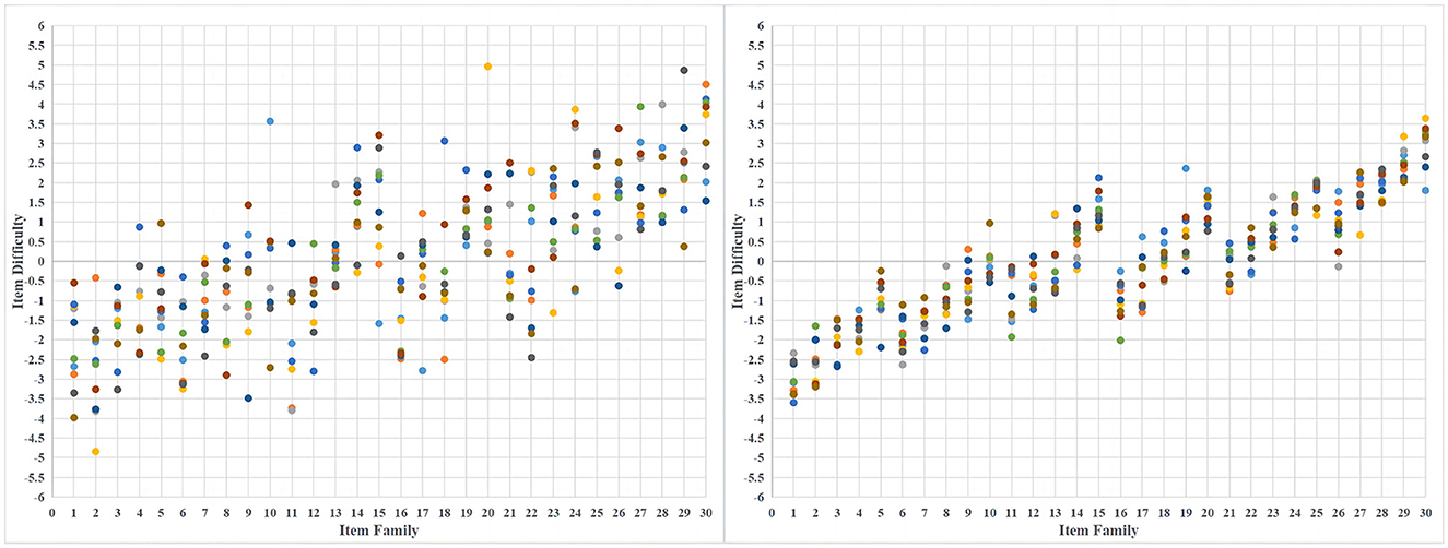
Figure 1. The simulated item difficulty distributions for R2 are 60% (left) and 90% (right).
Step 2: Simulation of examinees' abilities and scores
The number of examinees was set to 1,000, and each examinee's ability (θ) was drawn from a standard normal distribution N(0, 12).
The score matrix was generated using the RELLTM model. The correct response probability matrix for all item examinees is obtained by bringing the θ into the RELLTM model along with the item design parameters (ηk, qjk, and ej) from Step 1. Each value of this correct response probability matrix is then compared with a random number drawn from the uniform distribution Uniform(0, 1). When the value is greater than or equal to the random number, the element in the corresponding position of the score matrix is 1. Otherwise, it is 0. In this way, the score matrix is generated.
Step 3: Estimation of item difficulty in the item bank
Although the true value of item difficulty was known, this study aimed to compare the effects of different ways of calibrating (or predicting) item difficulty on the measurement efficiency in CAT. In other words, the item difficulty needs to be re-parameterized in the same situation. Therefore, the same score matrix obtained in Step 2 was given to five different item difficulty calibration (or prediction) approaches. These five approaches are USM, ISM, RSM, RELLTM, and LLTM, as mentioned in Section 2.2.
The hierarchical item family model and the cognitive IRT model are not the same. To unify the process of estimation algorithmically, this study used a Markov Chain Monte Carlo (MCMC) parameter estimation procedure via R and RStan. To ensure that each model converged sufficiently, the criterion for Rhat in this study was set to be < 1.05. In the case of 1,000 examinees and 300 items, two MCMC chains were set up, and each chain was run 10,000 times, with the mean of the last 5,000 taken as the parameter estimates. Since then, five-item difficulty parameters have been estimated and used for subsequent item selection.
Step 4: Simulation of the CAT process
The CAT simulation process was accomplished through the R program. First, the initial item was selected by randomly selecting a moderately difficult item (difficulty between −0.1 and 0.1) from the item bank. Then, the examinee's score on the initial item was found in the score matrix in Step 2. Afterward, the examinee ability estimate (θ) on the Rasch model was estimated using the expected a posteriori (EAP) estimation method.
Then, the loop of item selection and scoring was entered according to the five-item difficulty calibrations (or predictions) methods. For example, when using item difficulty calibrated through the USM model, a specific item selection strategy (e.g., Maximum Fisher Information) was used to select the item that best fits the examinee's current ability estimate. It should be noted that the item difficulty used in item selection is the calibrated (or predicted) item difficulty. After selecting an item, the examinee's score on that item was found in the score matrix in Step 2. The EAP method was then used to estimate on the Rasch model. In this way, the item selection and scoring loop were carried out.
Finally, the stopping rule of the loop was a fixed test length; that is, the test ended after a fixed number of test items (e.g., 60 items). The final estimate of θ on the Rasch model using the EAP method was used as the CAT estimate of this examinee's ability.
To compare the performance of the five calibration (or prediction) procedures (USM, ISM, RSM, RELLTM, and LLTM) under different item banks, the variables indicated above were kept constant, and the variable R2 was manipulated (60, 70, 80, and 90%).
The dependent variables are the recovery of theta and the measurement efficiency of CAT. RMSE was used to represent the recovery of theta in CAT. Measurement efficiency in this CAT was evaluated by determining the number of additional test items required to achieve the same RMSE achieved by the baseline model (USM/Rasch). To thoroughly examine these metrics, a total of 20 experimental conditions were formed and repeated 50 times for each experimental condition.
For the first research question, the variation of RMSE with test length is shown in Figure 2.
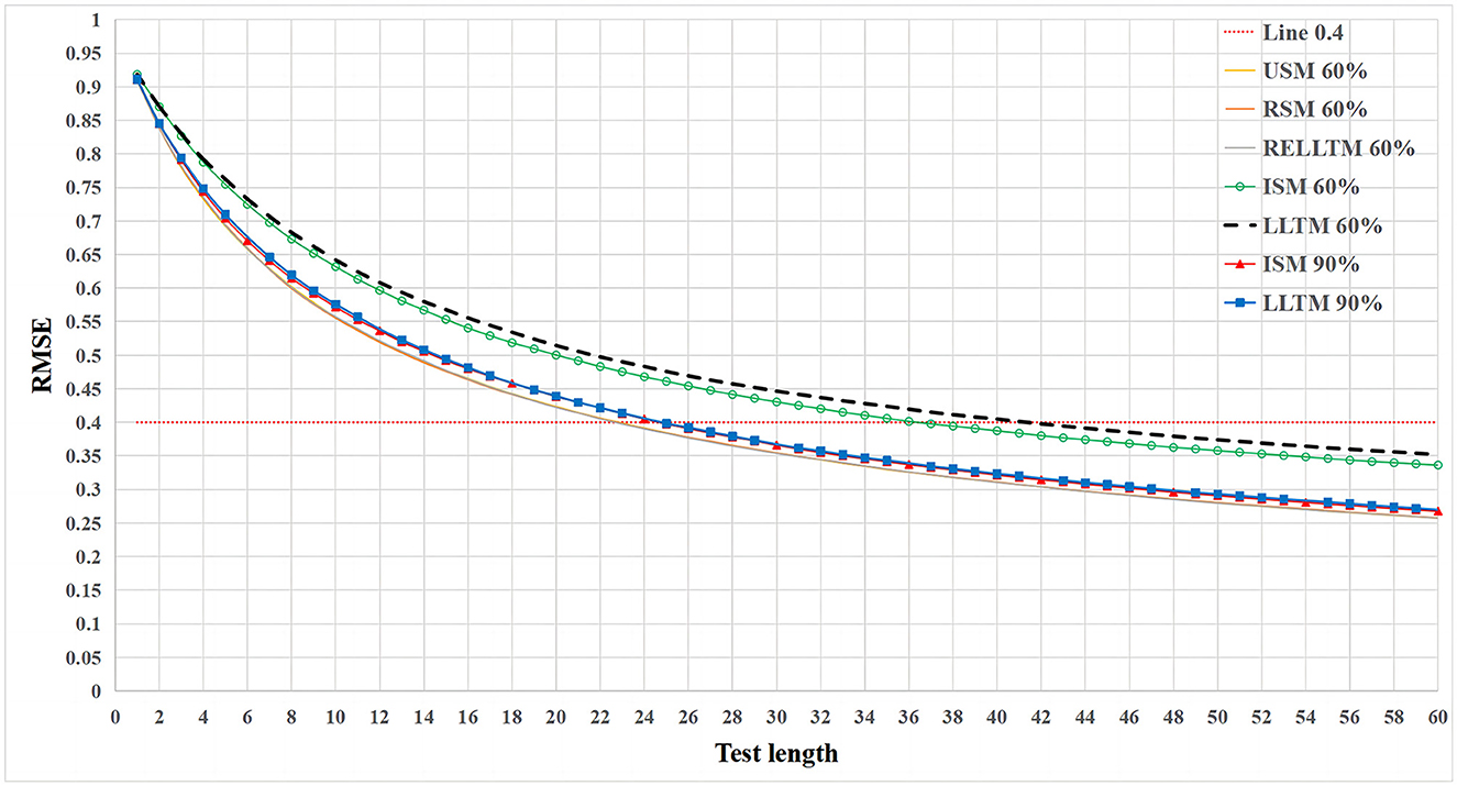
Figure 2. The variation of RMSE with test length for multiple experimental conditions at different R2.
Figure 2 only shows 7 of the 20 experimental conditions (USM 60%, RSM 60%, RELLTM 60%, ISM 60%, LLTM 60%, ISM 90%, and LLTM 90%). The appropriate simplification is made because the curves of USM, RSM, and RELLTM overlap for all four cases with an R2 of 60, 70, 80, and 90%. The remaining conditions (ISM 70%, LLTM 70%, ISM 80%, and LLTM 80%) were not painted for simplicity. Figure 2 shows that (1) the RMSE for USM, RSM, and RELLTM always remained equal, regardless of the level of the R2 and the test length and that (2) USM, RSM, and RELLTM are similar classes of curves, while ISM and LLTM are other classes. The RMSE of ISM and LLTM is always larger than other classes (USM, RSM, and RELLTM) regardless of test length, and the gap decreases as the R2 increases. When the R2 reaches 90%, the gap between the curves of the two classes is very small. (3) There is also a gap between ISM and LLTM, with LLTM having a higher RMSE than ISM, but the difference is not notable. In particular, the two curves overlap when the R2 increases to 90%.
More specifically, Table 1 demonstrates the RMSE when the test length is 30. A portion of the table shows the RMSE for the 20 experimental conditions, and the last two columns show the difference between the LLTM and the other two models in RMSE. Since each experimental design was repeated 50 times, differences between these models could be evaluated using ANOVA or independent sample t-tests. First, Table 1 also shows no difference between USM, RSM, and RELLTM in RMSE. Second, the independent sample t-test shows that the RMSE of LLTM is significantly higher than that of ISM when R2 = 60, 70, and 80%, but the difference with ISM is not significant when R2 = 90% (t = 0.935, p = 0.353, Cohen's d = 0.187). Finally, the independent sample t-test shows that the RMSE of LLTM is significantly higher than that of USM when R2 = 60, 70, 80, and 90%.
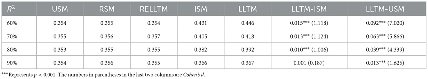
Table 1. RMSE and RMSE difference for five calibration (or prediction) methods at different R2.
For the second research question, the model of interest is the LLTM. As can be seen in Figure 2, the gap between RMSE under LLTM (predicted difficulty) and baseline model USM (calibrated difficulty) decreases as R2 increases. The LLTM is worse than USM in terms of RMSE, and the LLTM requires several additional items to achieve the same RMSE as USM. With the same RMSE criterion (RMSE = 0.4), the LLTM was compared to the baseline model (USM/Rasch), and Figure 3 shows the relationship between the number of additional items in CAT needed for the LLTM and the R2. Figure 3 describes a monotonically decreasing quadratic curve with the curve equation y = 100x2 – 206x + 106.5. If one wishes the test length of the CAT based on the predicted difficulty to be no more than 30 (including eight additional items), at least 75% of the R2 is needed.
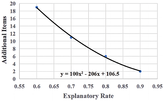
Figure 3. The relationship between the number of additional items and the R2 when RMSE = 0.4 is used as the criterion.
This study compared the effects of five-item calibration (or prediction) approaches on measurement efficiency in CAT. In response to the first research question, we obtained the following four conclusions: (1) These five approaches were divided into two categories in terms of measurement efficiency, and the first category (USM, RSM, and RELLTM) outperforms the second category (LLTM and ISM); (2) the RMSE of the first category does not vary with the R2. The RMSE of the second category decreases with R2, and the gap with the RMSE of the first category decreases accordingly; (3) in the second category (LLTM and ISM), ISM performs better on RMSE than LLTM; and (4) in response to the second research question, we conclude that the predictive model (LLTM) is worse than the baseline model (USM) in terms of RMSE, but the LLTM only needs a few more items to produce the same RMSE as the baseline model and that the number of additional items decreases as the R2 increases.
For Conclusion (1), USM, RSM, and RELLTM do not differ in RMSE because all three models have separate estimates of item difficulty, with RELLTM having separate estimates of the residual term ej for each item difficulty. In contrast, LLTM and ISM were only estimated at the item family level, and item difficulty within the item family was not estimated individually, which is simpler for the former category. Therefore, the first category is better than the second category in terms of measurement efficiency in CAT. Conclusion (2) is also in line with our expectations. As the R2 increases, it means that the data are increasingly consistent with the LLTM and ISM models, while the other three models are not affected by the R2 because they have separate estimates of item difficulty.
For conclusion (3), it is established that the LLTM is a generalized linear fixed-effects model in which item difficulty is predicted from item design variables. Therefore, in estimating item difficulty, compared to the ISM model, the LLTM model exhibits the phenomenon of regressing to the mean of the difficulty parameter of test items (regression to the mean). The degree of regression primarily depends on the validity of the item cognitive model and the quality of the item design features (Embretson, 1999). However, each item's difficulty was estimated separately in the ISM, so there is no phenomenon of “regression to the mean.” It is worth noting that the gap caused by this phenomenon of “regression to the mean” decreases as the R2 increases. A high R2 indicates that the difficulty of items within the item family tends to be more consistent. This finding means that the estimated regression coefficient for the item design variables in the LLTM is more stable and effective, leading to a more accurate prediction of item difficulty.
Conclusion (4) has significant value for item generation in CAT, especially for CAT, where items are generated on the fly. Item generation on the fly means that the items are generated instantaneously. Item difficulty can only be used with predictive difficulty. The results of the LLTM predictive difficulty tell us how many additional test items are needed in CAT to achieve the same RMSE as the baseline model or at least how much R2 is guaranteed to compensate for the loss of measurement efficiency from using predictive difficulty.
Finally, this study constructed a CAT item bank based on the CDS by means of simulation. The simulated item bank is not a substitute for a real-item bank, but the simulation approach allows for a wide variety of item bank situations to be easily obtained. We also used a real item bank for validation. All the items in this real item bank were mental rotation items measuring spatial ability, and the item bank was constructed using the CDS approach. The results under the real item bank are consistent with those under the simulated item bank.
With the advent of artificial intelligence (AI), item generation based on AI will become more and more common. However, this is only a technological advancement; validity is still key to item generation. Validity involves theoretical thinking about the construct, which is difficult to achieve with the current form of AI. Recent studies have used GPT for item generation for personality items (Hommel et al., 2022), which is more like a weak-theory item generation approach, and item generation methods that combine GPT with a cognitive design system approach still need to be developed. In conclusion, CAT based on the CDS approach is highly promising and practical. It combines cognitive psychology, psychometrics, and computer science and is one of the future directions of the new generation of AI assessment.
The raw data supporting the conclusions of this article will be made available by the authors, without undue reservation.
HL: Writing – original draft, Writing – review & editing. XY: Writing – review & editing.
The author(s) declare that no financial support was received for the research, authorship, and/or publication of this article.
The authors declare that the research was conducted in the absence of any commercial or financial relationships that could be construed as a potential conflict of interest.
All claims expressed in this article are solely those of the authors and do not necessarily represent those of their affiliated organizations, or those of the publisher, the editors and the reviewers. Any product that may be evaluated in this article, or claim that may be made by its manufacturer, is not guaranteed or endorsed by the publisher.
The Supplementary Material for this article can be found online at: https://www.frontiersin.org/articles/10.3389/fpsyg.2024.1353419/full#supplementary-material
Embretson, S. E. (1998). A cognitive design system approach to generating valid tests: application to abstract reasoning. Psychol. Methods 3, 380–396. doi: 10.1037/1082-989X.3.3.380
Embretson, S. E. (1999). Generating items during testing: Psychometric issues and models. Psychometrika 64, 407–433. doi: 10.1007/BF02294564
Embretson, S. E., and Yang, X. (2007). “Automatic item generation and cognitive psychology,” in Handbook of Statistics: Psychometrics, Volume 26, eds. C. R. Rao, and S. Sinharay (Amsterdam: Elsevier), 747–768.
Hommel, B. E., Wollang, F. M., Kotova, V., Zacher, H., and Schmukle, S. C. (2022). Transformer-based deep neural language modeling for construct-specific automatic item generation. Psychometrika 87, 749–772. doi: 10.1007/s11336-021-09823-9
Janssen, R., Schepers, J., and Peres, D. (2004). “Models with item and item group predictors,” in Explanatory Item Response Models: A Generalized Linear and Nonlinear Approach, eds. P. de Boeck, and M. Wilson (New York, NY: Springer-Verlag).
Luecht, R. M. (2012). “Automatic item generation for computerized adaptive testing,” in Automatic Item Generation: Theory and Practice, eds. M. J. Gierl, and T. M. Haladyna (London; New York, NY: Routledge), 196–216.
Millman, J., and Westman, R. S. (1989). Computer-assisted writing of achievement test items: toward a future technology. J. Educ. Meas. 26, 177–190. doi: 10.1111/j.1745-3984.1989.tb00327.x
Sinharay, S., Johnson, M. S., and Williamson, D. M. (2003). Calibrating item families and summarizing the results using family expected response functions. J. Educ. Behav. Stat. 28, 295–313. doi: 10.3102/10769986028004295
Keywords: computerized adaptive testing, cognitive design system approach, item bank, item generation, linear logistic trait model
Citation: Luo H and Yang X (2024) Efficiency of computerized adaptive testing with a cognitively designed item bank. Front. Psychol. 15:1353419. doi: 10.3389/fpsyg.2024.1353419
Received: 10 December 2023; Accepted: 10 June 2024;
Published: 26 June 2024.
Edited by:
Ioannis Tsaousis, National and Kapodistrian University of Athens, GreeceReviewed by:
Mark D. Reckase, Michigan State University, United StatesCopyright © 2024 Luo and Yang. This is an open-access article distributed under the terms of the Creative Commons Attribution License (CC BY). The use, distribution or reproduction in other forums is permitted, provided the original author(s) and the copyright owner(s) are credited and that the original publication in this journal is cited, in accordance with accepted academic practice. No use, distribution or reproduction is permitted which does not comply with these terms.
*Correspondence: Xiangdong Yang, eGR5YW5nNTBAaG90bWFpbC5jb20=
Disclaimer: All claims expressed in this article are solely those of the authors and do not necessarily represent those of their affiliated organizations, or those of the publisher, the editors and the reviewers. Any product that may be evaluated in this article or claim that may be made by its manufacturer is not guaranteed or endorsed by the publisher.
Research integrity at Frontiers
Learn more about the work of our research integrity team to safeguard the quality of each article we publish.