Exploration and analysis of a generalized one-parameter item response model with flexible link functions

This paper primarily analyzes the one-parameter generalized logistic (1PGlogit) model, which is a generalized model containing other one-parameter item response theory (IRT) models. The essence of the 1PGlogit model is the introduction of a generalized link function that includes the probit, logit, and complementary log-log functions. By transforming different parameters, the 1PGlogit model can flexibly adjust the speed at which the item characteristic curve (ICC) approaches the upper and lower asymptote, breaking the previous constraints in one-parameter IRT models where the ICC curves were either all symmetric or all asymmetric. This allows for a more flexible way to fit data and achieve better fitting performance. We present three simulation studies, specifically designed to validate the accuracy of parameter estimation for a variety of one-parameter IRT models using the Stan program, illustrate the advantages of the 1PGlogit model over other one-parameter IRT models from a model fitting perspective, and demonstrate the effective fit of the 1PGlogit model with the three-parameter logistic (3PL) and four-parameter logistic (4PL) models. Finally, we demonstrate the good fitting performance of the 1PGlogit model through an analysis of real data.

1. Introduction

Latent trait models, also known as item response theory (IRT) models, have gained widespread application in educational testing and psychological measurement (Lord and Novick, 1968; van der Linden and Hambleton, 1997; Embretson and Reise, 2000; Baker and Kim, 2004). These models utilize the probability of a response to establish the interaction between an examinee's “ability” and the characteristics of the test items, such as difficulty and guessing. The focus is on analyzing the pattern of responses rather than relying on composite or total score variables and linear regression theory. Specifically, IRT aims to model students' ability by examining their performance at the question level, providing a granular perspective on each student's ability based on the unique insights each question offers.

The Rasch model, also known as the one-parameter logistic IRT model, was innovated by Georg Rasch in 1960 and serves as a strategic tool in psychometrics for evaluating categorical data. This data includes responses to reading exams or survey questions and is analyzed in correlation with the trade-off between the respondent's ability, attitude, or personality trait and the item's difficulty (Rasch, 1960). For instance, this model could be used to determine a student's level of reading comprehension or gauge the intensity of a person's stance on issues like capital punishment from their questionnaire responses. Beyond the realms of psychometrics and educational research, the Rasch model and its derivatives also find applications in diverse fields such as healthcare (Bezruczko, 2005), market research (Wright, 1977; Bechtel, 1985), and agriculture (Moral and Rebollo, 2017).

Within the framework of the Rasch model, the probability of a specific response–such as right or wrong–is modeled in relation to the examinee's ability and the item characteristic. Particularly, the classical Rasch model models the probability of a correct response as a logistic function of the discrepancy between the examinee's ability and the item difficulty. Typically, the model parameters depict the proficiency level of examinees and the complexity level of the items on a continuous latent scale. For instance, in educational assessments, the item parameter illustrates the difficulty level, whereas the person parameter represents the ability or attainment level of the examinee. The higher an individual's ability relative to the item difficulty, the higher the probability of a correct response. In cases where an individual's ability position equals the item difficulty level, the Rasch model inherently predicts a 50% chance of a correct response.

Parallel to the logistic IRT models, the normal ogive IRT models utilize the probit function to delineate the relationship between ability and item response, whereas the logistic IRT model employs the logit function to depict the same relationship. This constitutes a fundamental difference between the normal ogive IRT models and the more frequently utilized logistic IRT models. In fact, the use of the normal ogive model in the testing context has been further developed by a number of researchers. Lawley (1943, 1944) was the first to formally employ the normal ogive model to directly model binary item response data. Tucker (1946) used the term “item curve” to indicate the relationship between item response and ability. The early attempts at modeling binary response data culminated in the work of Lord (1952, 1953, 1980) who, unlike the early researchers, treated ability as a latent trait to be estimated and in doing so, laid the foundation for IRT.

The normal ogive IRT models (Lord, 1980; van der Linden and Hambleton, 1997; Embretson and Reise, 2000; Baker and Kim, 2004), also known as the one parameter normal ogive model, are a mathematical model used in the field of psychometrics to relate the latent ability of an examinee to the probability of a correct response on a test item. This model, as a component of IRT, facilitates the design, analysis, and scoring of tests, questionnaires, and comparable instruments intended for the measurement of abilities, attitudes, or other variables.

As previously noted, the Rasch model and the one-parameter normal ogive IRT model are premised upon symmetric functions to delineate the relationship between ability and item response, which result in a symmetric ICC. However, in certain contexts, these symmetric IRT models may not sufficiently capture the characteristics inherent in the data. These situations necessitate the utilization of asymmetric IRT models. Several asymmetric IRT models currently exist, such as the non-parametric Bayesian model, which constructs the ICC with a Dirichlet process prior (Qin, 1998; Duncan and MacEachern, 2008), and the Bayesian beta-mixture IRT model (BBM-IRT), which models the ICC with a flexible finite mixture of beta distribution (Arenson and Karabatsos, 2018). Karabatsos (2016) used the infinite mixture of normal c.d.f to model ICC, while Luzardo and Rodriguez (2015) constructed the ICC using the kernel regression method. There are also some skewed logistic IRT models, such as the logistic positive exponent (LPE) model and the reflection LPE (RLPE) model (Samejima, 1997, 1999, 2000; Bolfarine and Bazan, 2010; Zhang et al., 2022), which utilize skewed modifications of the logit links. Moreover, the positive trait item response model (PTIRM), which employs the log-logistic, lognormal, and Weibull as link functions to link the latent trait to the response, is used in some literature (Lucke, 2014; Magnus and Liu, 2018). In addition, the one-parameter complementary log-log IRT model also yields an asymmetric ICC (Goldstein, 1980; Shim et al., 2022). Compared to their symmetric counterparts, asymmetric IRT models can encapsulate a wider spectrum of data characteristics, particularly when the speed at which the probability of a positive response changes varies across different intervals of the latent trait. Furthermore, asymmetric IRT models are better suited to accommodate data where the probability of a positive response escalates more rapidly at higher trait levels and increases more sluggishly at lower trait levels. These asymmetric models, therefore, have a distinct advantage in capturing the nuanced dynamics of item responses that do not adhere strictly to symmetric patterns, thereby providing a more accurate representation of the interplay between individual ability and item response. As such, they represent a crucial development within the IRT field, broadening the applicability of these models in psychometric analyses and educational measurement.

This article discusses and analyzes the aforementioned one-parameter IRT models: the Rasch model, the one-parameter normal ogive IRT model, and the one-parameter complementary log-log IRT model. We propose a unified model representation that can encompass all three models through the manipulation of specific parameter values. In the present paper, our emphasis is placed on a class of generalized logistic models, introduced initially by Stukel (1988). This class of link functions is guided by a duo of parameters, precisely (η₁, η₂). By modulating the values of (η₁, η₂), this class is inclusive of logit, probit, complementary log-log link, along with an assortment of other symmetric and asymmetric links as particular instances. This class of models boasts sufficient versatility to accommodate the fitting of identical or diverse links to distinct items nested within the IRT model framework. An additional appealing characteristic of this class streamlines the execution of Markov chain Monte Carlo (MCMC) sampling from the posterior distribution via the recently formulated software, Stan. This research paper encompasses several key aspects. Firstly, we thoroughly discuss symmetric models such as the logit and probit models, as well as asymmetric models like the complementary log-log and generalized logit models, within the framework of a one-parameter IRT model. Secondly, we employ different links for different items in our analysis. Thirdly, we utilize the Stan platform to implement this flexible range of links for one parameter models and provide the corresponding Stan codes. By leveraging Stan, we are able to calculate deviance information criterion (DIC; Spiegelhalter et al., 2002) based on posterior distribution samples, which can naturally guide the selection of links and IRT model types. Lastly, through the 2015 computer-based PISA (Program for International Student Assessment) sciences data, we empirically demonstrate that employing different generalized logit links for different items markedly improves data fit compared to traditional logistic, normal ogive and complementary log-log models, as determined by DIC criteria.

The remainder of this paper is organized as follows. In Section 2, we review the three one-parameter IRT models and the generalized logit link function, then introduce the main model of our study, namely the one-parameter generalized logistic (1PGlogit) model. In Section 3, we describe the Bayesian parameter estimation method that we use, discuss its software implementation, and elaborate on the Bayesian model assessment criteria we employ to evaluate the model fittings. Section 4 presents three simulation studies aimed at exploring the accuracy of model parameter estimation and assessing the fit of the 1PGlogit model in relation to various other symmetric or asymmetric models. In Section 5, we conduct an empirical study to validate the practical utility of the 1PGlogit model. Finally, in Section 6, we provide a summary of the paper.

2. Item response theory models with generalized logistic link functions

2.1. Overview of the one-parameter IRT models

The initial model in the field of IRT can be traced back to the 1930s, as proposed by Ferguson (1942), Lawley (1943), Mosier (1940, 1941), and Richardson (1936). It was later improved by Lord and Novick (1968) into what is now commonly referred to as the normal ogive model. Suppose we have N students each answering J items. Let X denote the response variable, and let x_ij be the response of the ith student (i = 1, ⋯  , N) on the jth item (j = 1, ⋯  , J). Here, x_ij = 1 indicates a correct answer, and x_ij = 0 indicates an incorrect one. Within the one-parameter normal ogive (1PNO) model, the probability of a correct response by the ith student on the jth item can be expressed as follows:

$\begin{array}{ll}P(x_{ij}=1|{\theta }_i,{\beta }_j)={\displaystyle {\int }_{-\infty }^{{\theta }_i-{\beta }_j}}\frac{1}{\sqrt{2\pi }}{e}^{-\frac{z^2}{2}}dz.& (1)\end{array}$

Here, β_j is the difficulty parameter of the jth item and θ_i is the latent trait of the ith student. A larger β_j implies a more difficult item, and the probability of a correct response increases with the increasing value of θ_i. As we can see, the 1PNO model is essentially a generalized linear model with a probit link.

Although the 1PNO model is quite interpretable and intuitive, its computation is complicated. In response to this, Rasch proposed the Rasch model in 1960, which was essentially a generalized linear model with a logit link. Specifically, the probability of a correct response in the model can be expressed in the following form:

$\begin{array}{ll}P(x_{ij}=1|{\theta }_i,{\beta }_j)=\frac{exp({\theta }_i-{\beta }_j)}{1+exp({\theta }_i-{\beta }_j)},& (2)\end{array}$

where β_j and θ_i maintain the same interpretations as in the 1PNO model. In this form, to describe the probability of a student's response, it is no longer necessary to compute the cumbersome integrals, thereby simplifying the calculation.

Both of the models mentioned above possess a symmetrical item characteristic curve (ICC). However, Shim et al. (2022) proposed a one-parameter complementary log-log model (CLLM) which exhibits an asymmetric ICC. The probability of a correct response in the CLLM model can be expressed as follows:

$\begin{array}{ll}P(x_{ij}=1|{\theta }_i,{\beta }_j)=1-exp\left\{-exp({\theta }_i-{\beta }_j)\right\},& (3)\end{array}$

where β_j and θ_i retain the same interpretations as in the two models discussed earlier. As demonstrated by Shim et al. (2022), the CLLM possesses the capability to effectively address the guessing behavior exhibited by examinees in the three-parameter logistic (3PL) model and, in certain cases, can yield even better results. This implies that CLLM accounts for the effect of guessing. Essentially, the CLLM is a generalized linear model with a complementary log-log link.

2.2. Overview of the family of models based on generalized logit links

Let y be a dichotomous random variable. We assume that y equals 1 with probability μ(η) and 0 with probability 1 − μ(η), where η is a linear predictor. Stukel (1988) introduced a class of generalized logistic models (Glogits), indexed by two shape parameters λ = (λ₁, λ₂). Therefore, the Glogits model is controlled by a strictly increasing non-linear function h_λ (η). The specific expression is as follows:

$\begin{array}{ll}\mu (\eta )=\frac{\exp \left\{h_{\lambda }\left(\eta \right)\right\}}{1+\exp \left\{h_{\lambda }\left(\eta \right)\right\}},& (4)\end{array}$

where the function h_λ (η) is defined as follows:

for η > 0 $(\mu (\eta )>\frac{1}{2})$,

$\begin{array}{ll}{h}_{\lambda }\left(\eta \right)=\{\begin{array}{cc}-\frac{\log (1-{\lambda }_1\eta )}{{\lambda }_1},& {\lambda }_1<\text{0},\\ \eta ,& {\lambda }_1=\text{0},\\ \frac{\exp \left({\lambda }_1\eta \right)-1}{{\lambda }_1},& {\lambda }_1>\text{0}.\end{array}& (5)\end{array}$

for η ≤ 0 $(\mu (\eta )\le \frac{1}{2})$,

$\begin{array}{ll}{h}_{\lambda }\left(\eta \right)=\{\begin{array}{cc}\frac{\log (1-{\lambda }_2|\eta |)}{{\lambda }_2},& {\lambda }_2<\text{0},\\ \eta ,& {\lambda }_2=\text{0},\\ -\frac{\exp \left({\lambda }_2|\eta |\right)-1}{{\lambda }_2},& {\lambda }_2>\text{0}.\end{array}& (6)\end{array}$

As evident from the above equations, the logit link serves as a special case of Glogits when λ₁ = λ₂ = 0. Furthermore, Stukel (1988) revealed that Glogits can be simplified to several other link functions under certain conditions. For instance, it reduces to a probit link when λ₁ = λ₂ ≈ 0.165, a log-log link when λ₁ ≈ −0.037 and λ₂ ≈ 0.62, a complementary log-log link when λ₁ ≈ 0.62 and λ₂ ≈ −0.037, and a Laplace link when λ₁ = λ₂ ≈ −0.077.

2.3. One-parameter generalized logistic IRT model

According to Glogit models, μ(η) forms a cumulative distribution function for η, which can be interpreted as the probability of a correct answer in IRT. Building on the traditional difficulty and ability parameters in a one-parameter IRT model, we reintroduce two shape parameters related to the item factors, denoted as λ_j = (λ_1j, λ_2j). Consequently, we can deduce that the one-parameter generalized logistic model (1PGlogit) can be articulated as follows:

$\begin{array}{ll}P(x_{ij}=1|{\theta }_i,{\beta }_j,{\lambda }_j)=\frac{exp\left\{h_{{\lambda }_j}({\theta }_i-{\beta }_j)\right\}}{1+exp\left\{h_{{\lambda }_j}({\theta }_i-{\beta }_j)\right\}}.& (7)\end{array}$

Furthermore, when θ_i − β_j > 0 (which implies that $P(x_{ij}=1|{\theta }_i,{\beta }_j,{\lambda }_j)>\frac{1}{2}$),

$\begin{array}{ll}{h}_{{\lambda }_j}\left({\theta }_i-{\beta }_j\right)=\{\begin{array}{cc}-\frac{\log (1-{\lambda }_{1j}({\theta }_i-{\beta }_j))}{{\lambda }_{1j}},& {\lambda }_{1j}<\text{0,}\\ {\theta }_i-{\beta }_j,& {\lambda }_{1j}=\text{0},\\ \frac{\exp \left({\lambda }_{1j}({\theta }_i-{\beta }_j)\right)-1}{{\lambda }_{1j}},& {\lambda }_{1j}>\text{0}.\end{array}& (8)\end{array}$

When θ_i − β_j ≤ 0, which implies that ($P(x_{ij}=1|{\theta }_i,{\beta }_j,{\lambda }_j)\le \frac{1}{2}$),

$\begin{array}{ll}{h}_{{\lambda }_j}\left({\theta }_i-{\beta }_j\right)=\{\begin{array}{cc}\frac{\log (1-{\lambda }_{2j}|{\theta }_i-{\beta }_j|)}{{\lambda }_{2j}},& {\lambda }_{2j}<\text{0,}\\ {\theta }_i-{\beta }_j,& {\lambda }_{2j}=\text{0},\\ -\frac{\exp \left({\lambda }_{2j}|{\theta }_i-{\beta }_j|\right)-1}{{\lambda }_{2j}},& {\lambda }_{2j}>\text{0}.\end{array}& (9)\end{array}$

Specifically, when λ_1j = λ_2j = 0, the 1PGlogit model reduces to the Rasch model as shown in Equation (2); when λ_1j = λ_2j ≈ 0.165, the 1PGlogit model becomes the traditional 1PNO model in Equation (1). This applies when θ_i − β_j ≤ 0, we have

$\begin{array}{ll}P(x_{ij}=1|{\theta }_i,{\beta }_j)=\frac{exp\left\{-\frac{exp\{0.165|{\theta }_i-{\beta }_j|\}-1}{0.165}\right\}}{1+exp\left\{-\frac{exp\{0.165|{\theta }_i-{\beta }_j|\}-1}{0.165}\right\}},& (10)\end{array}$

when θ_i − β_j > 0, we have

$\begin{array}{ll}P(x_{ij}=1|{\theta }_i,{\beta }_j)=\frac{exp\left\{\frac{exp\{0.165({\theta }_i-{\beta }_j)\}-1}{0.165}\right\}}{1+exp\left\{\frac{exp\{0.165({\theta }_i-{\beta }_j)\}-1}{0.165}\right\}},& (11)\end{array}$

In fact, the CLLM model in Equation (3) is also a special case of the 1PGlogit model when the two shape parameters are restricted to λ_1j ≈ 0.62 and λ_2j ≈ −0.037. Specifically, when θ_i − β_j ≤ 0,

$\begin{array}{ll}P(x_{ij}=1|{\theta }_i,{\beta }_j)=\frac{exp\left\{-\frac{log\{1+0.037|{\theta }_i-{\beta }_j|\}}{0.037}\right\}}{1+exp\left\{-\frac{log\{1+0.037|{\theta }_i-{\beta }_j|\}}{0.037}\right\}},& (12)\end{array}$

when θ_i − β_j > 0,

$\begin{array}{ll}P(x_{ij}=1|{\theta }_i,{\beta }_j)=\frac{exp\left\{\frac{exp\{0.62({\theta }_i-{\beta }_j)\}-1}{0.62}\right\}}{1+exp\left\{\frac{exp\{0.62({\theta }_i-{\beta }_j)\}-1}{0.62}\right\}},& (13)\end{array}$

To intuitively explore 1PGlogit IRT models, we visualize the ICCs of 1PGlogit IRT models with different λ_1j and λ_2j in Figure 1, where the difficulty parameter b is set as 0. It can be observed from Figure 1 that parameters λ_1j and λ_2j control the convergence speed of the tail of 1PGlogit. The speed at which the tail of the ICC approaches 0 can be referred to as the “rate of convergence to the lower limit”. Similarly, the speed at which the ICC approaches 1 can be referred to as the “rate of convergence to the upper limit”. Specifically, Figure 1A shows that the parameter λ_1j controls the convergence speed to the upper asymptote, while Figure 1B shows that the parameter λ_2j controls the convergence speed to the lower asymptote. Common to both parameters is that the larger the value of λ_1j (λ_2j), the faster the ICCs converge to the upper (lower) asymptote line. For instance, as shown in Figure 1A, when λ_1j = 1, the ICC of 1PGlogit(1, 0)has already converged to the upper asymptote P(θ) = 1 before θ = 2, while when λ_1j = 0, the ICC of 1PGlogit(0, 0) (i.e., Rasch model) just reaches the upper asymptote at θ = 4. However, when λ_1j = −1, the ICC of 1PGlogit(−1, 0) only converges to around P(θ) = 0.8 at θ = 4. The effect of the parameter λ_2j on the convergence of the ICC to the lower asymptote is similar to that of λ_1j, which can be seen in Figure 1B.

FIGURE 1

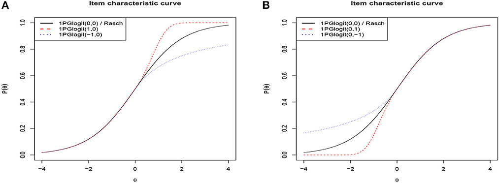
Figure 1. Item characteristic curves based on different the 1PGlogit models. (A) β_j = 0, λ_1j = 0, 1, −1 and λ_2j = 0. (B) β_j = 0, λ_1j = 0 and λ_2j = 0, 1, −1.

Based on the above analysis, it can be seen that the role of the parameter λ_j in 1PGlogit is somewhat analogous to the parameter c in the three-parameter logistic (3PL) model and the parameter d in the four-parameter logistic (4PL) model. As a result, we further compared the ICC of 1PGlogit with that of the 3PL model in Figure 2A and with the 4PL model in Figure 2B. Specifically, the expressions for the 3PL and 4PL models are as follows:

$\begin{array}{ll}P(x_{ij}=1|{\theta }_i,{\alpha }_j,{\beta }_j,c_j)=c_j+(1-c_j)\frac{exp\{{\alpha }_i({\theta }_i-{\beta }_j)\}}{1+exp\{{\alpha }_i({\theta }_i-{\beta }_j)\}},& (14)\end{array}$

and

$\begin{array}{ll}P(x_{ij}=1|{\theta }_i,{\alpha }_j,{\beta }_j,c_j,d_j)=c_j+(d_j-c_j)\frac{exp\{{\alpha }_i({\theta }_i-{\beta }_j)\}}{1+exp\{{\alpha }_i({\theta }_i-{\beta }_j)\}}.& (15)\end{array}$

In these models, α_j is the discrimination parameter, c_j is the lower asymptote parameter (which can be viewed as a guessing probability), and d_j is the upper asymptote parameter, where 1 − d_j can be considered as a slipping probability. For this analysis, we set α_j = 1, β_j = 0, c_j = 0.2, and d_j = 0.8. As demonstrated in Figure 2A, the 3PL model has an upper asymptote at P(θ) = 1 and a lower asymptote at P(θ) = 0.2, while the 1PGlogit(0, −1), with λ_1j = 0 and λ_2j = −1, displays an ICC similar to that of the 3PL model. In Figure 2B, the 4PL model exhibits an upper asymptote at P(θ) = 0.8 and a lower asymptote at P(θ) = 0.2. When λ_1j = −1 and λ_2j = −1, the 1PGlogit(−1, −1) shows an ICC comparable to the 4PL model. Hence, the parameter λ_j in 1PGlogit can be adjusted to represent the assumed guessing and slipping behaviors in the 3PL and 4PL models.

FIGURE 2

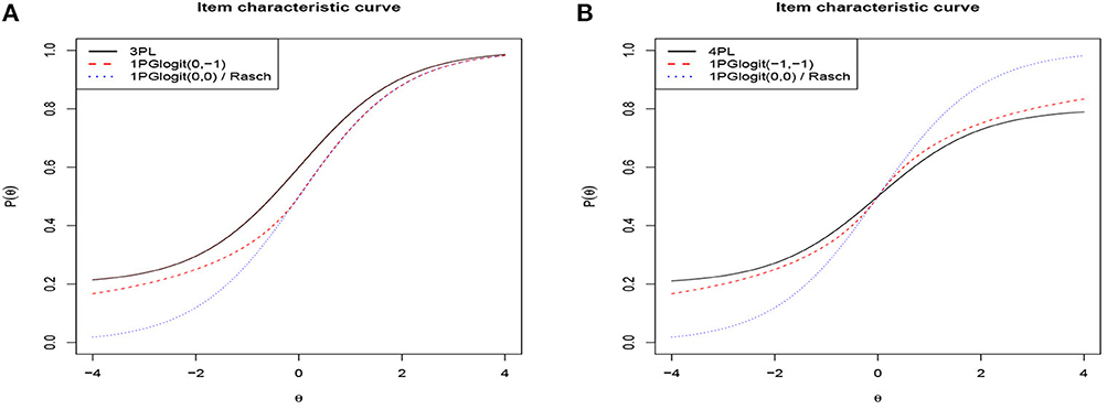
Figure 2. Item characteristic curves based on 3PL, 4PL, and 1PGlogit models. (A) 3PL model with α_j = 1, β_j = 0, c_j = 0.2. (B) 4PL model with α_j = 1, β_j = 0, c_j = 0.2, d_j = 0.8.

3. Bayesian estimation and model evaluations

In this study, we adopt the Bayesian statistical inference method to estimate the parameters in 1PGlogit IRT models. Let P_ij = p(x_ij = 1|β_j, λ_1j, λ_2j, θ_i), which is defined as shown in Equations (7)–(9). Thus, the likelihood function for the response of the ith examinee to the jth item can be written as:

$\begin{array}{ll}p(x_{ij}|{\beta }_j,{\lambda }_{1j},{\lambda }_{2j},{\theta }_i)=P_{ij}^{x_{ij}}{(1-P_{ij})}^{1-x_{ij}}.& (16)\end{array}$

Let x = (x_i, ⋯  , x_N), β = (β₁, ⋯  , β_J), λ₁ = (λ₁₁, ⋯  , λ_1J), λ₂ = (λ₂₁, ⋯  , λ_2J), θ = (θ₁, ⋯  , θ_N). Then the joint posterior distribution of parameters β, λ₁, λ₂, and θ can be derived as:

$\begin{array}{ll}\begin{array}{c}p(\beta ,{\lambda }_1,{\lambda }_2,\theta |x)=p(x|\beta ,{\lambda }_1,{\lambda }_2,\theta )p(\beta )p({\lambda }_1)p({\lambda }_2)p(\theta ),\hfill \\ ={\displaystyle \underset{\text{Likelihood function}}{{\displaystyle \underbrace{\left\{{\displaystyle \prod _{i=1}^N}{\displaystyle \prod _{j=1}^J}p(x_{ij}|{\beta }_j,{\lambda }_{1j},{\lambda }_{2j},{\theta }_i)\right\}}}}}{\displaystyle \underset{\text{Prior distributions}}{{\displaystyle \underbrace{\left\{{\displaystyle \prod _{j=1}^J}p({\beta }_j)p({\lambda }_{1j})p({\lambda }_{2j})\right\}\left\{{\displaystyle \prod _{i=1}^N}p({\theta }_i)\right\}}}}}.\end{array}& (17)\end{array}$

3.1. Prior distributions

According to Chen et al. (2002) and Chen et al. (1999), it is necessary to constrain the parameters λ_1j and λ_2j to be greater than −1 to ensure a proper posterior distribution. Therefore, the priors for λ_1j and λ_2j should be truncated at −1. The parameters β_j and θ_i are assumed to follow different normal prior distributions, while λ_1j and λ_2j are assumed to follow a truncated normal prior distribution. Overall, the priors for the parameters are set as follows:

$\begin{array}{ll}\begin{array}{c}{\beta }_j~\text{N}(0,{\sigma }_{\beta }^2),\hfill \\ {\lambda }_{1j}~\text{N}(0,{\sigma }_{\lambda }^2)\mathcal{I}(-1,\infty ),\hfill \\ {\lambda }_{2j}~\text{N}(0,{\sigma }_{\lambda }^2)\mathcal{I}(-1,\infty ),\hfill \\ {\theta }_i~\text{N}(0,1),\hfill \\ {\sigma }_{\beta }~\text{Cauchy}(0,5)\mathcal{I}(0,\infty ),\hfill \\ {\sigma }_{\lambda }~\text{Cauchy}(0,5)\mathcal{I}(0,\infty ),\hfill \end{array}\hfill & (18)\end{array}$

where $\mathcal{I}(a,b)$ implies that the parameter is constrained within the interval (a, b).

3.2. Stan software

In this paper, we employ the MCMC method for parameter estimation. Currently, there are various software options available for implementing the MCMC algorithm, such as WinBUGS (Lunn et al., 2000), OpenBUGS (Spiegelhalter et al., 2010), and JAGS (Plummer, 2003). However, In the subsequent research, we utilize the Stan software (Stan Development Team, 2019), which is based on the Hamiltonian Monte Carlo (HMC) algorithm (Neal, 2011) and the no-U-turn sampler (NUTS) (Hoffman and Gelman, 2014). HMC efficiently explores posteriors in models and is often faster than the Gibbs method (Geman and Geman, 1984) and the Metropolis algorithm (Metropolis et al., 1953), while NUTS further improves efficiency. Additionally, Stan provides interfaces with data analysis languages such as R, Python, Matlab, etc., making it convenient for our use. To implement the Stan program, we specifically utilize the R package rstan, which interfaces with Stan in R (R Core Team, 2019). The Stan code employed for parameter estimation in this study, along with the actual data, can be found at the following URL: https://github.com/X-Wang777/-A-Generalized-One-Parameter-IRT. Furthermore, Luo and Jiao (2018) offer a detailed tutorial on utilizing Stan for estimating various IRT models.

3.3. Criteria for assessing parameter estimation accuracy

In this research, we will use four criteria for assessing the accuracy of parameter estimation. They are Bias, RMSE (Root Mean Squared Error), SE (Standard Error), and SD (Standard Deviation). Assuming the parameter of interest is β_j, the evaluation criteria based on the β_j parameter are defined as follows:

$\begin{array}{c}\text{ Bias}({\beta }_j)=\frac{1}{R}{\displaystyle \sum _{r=1}^R}({\hat{\beta }}_j^{(r)}-{\beta }_j),\hfill \\ \text{RMSE}({\beta }_j)=\sqrt{\frac{1}{R}{\displaystyle \sum _{r=1}^R}{({\hat{\beta }}_j^{(r)}-{\beta }_j)}^2},\hfill \\ \text{ SE}({\beta }_j)=\sqrt{\frac{1}{R}{\displaystyle \sum _{r=1}^R}{\left({\hat{\beta }}_j^{(r)}-\frac{1}{R}{\displaystyle \sum _{l=1}^R}{\hat{\beta }}_j^{(l)}\right)}^2},\hfill \\ \text{ SD}({\beta }_j)=\frac{1}{R}{\displaystyle \sum _{r=1}^R}S{D}^{(r)}({\beta }_j).\hfill \end{array}$

where R denotes the number of replications and ${\hat{\beta }}_j^{(r)}$ is the estimate of β_j in the rth replication, and ${\mathrm{\text{SD}}}^{(r)}({\beta }_j)$ is the posterior standard deviation of β_j in the rth replication. Thus, we are able to calculate the average values for the four accuracy assessment indicators based on all items. That is,

$\begin{array}{c}\text{ Average Bias}(\beta )=\frac{1}{J\times R}{\displaystyle \sum _{j=1}^J}{\displaystyle \sum _{r=1}^R}({^}_j^{(r)}-{\beta }_j),\hfill \\ \text{Average RMSE}(\beta )=\frac{1}{J}{\displaystyle \sum _{j=1}^J}\sqrt{\frac{1}{R}{\displaystyle \sum _{r=1}^R}{({\hat{\beta }}_j^{(r)}-{\beta }_j)}^2},\hfill \\ \text{ Average SE}(\beta )=\frac{1}{J}{\displaystyle \sum _{j=1}^J}\sqrt{\frac{1}{R}{\displaystyle \sum _{r=1}^R}{\left({\hat{\beta }}_j^{(r)}-\frac{1}{R}{\displaystyle \sum _{l=1}^R}{\hat{\beta }}_j^{(l)}\right)}^2},\hfill \\ \text{ Average SD}(\beta )=\frac{1}{J\times R}{\displaystyle \sum _{j=1}^J}{\displaystyle \sum _{r=1}^R}S{D}^{(r)}({\beta }_j).\hfill \end{array}$

3.4. Bayesian model assessment

The following four model selection criteria will be used in this paper to evaluate the goodness of model fit: (1) DIC, (2) Logarithm of the pseudomarginal Likelihood (LPML; Geisser and Eddy, 1979; Ibrahim et al., 2001), (3) Widely applicable information criterion (WAIC; Watanabe and Opper, 2010), and (4) Leave-one-out cross-validation (LOO; Vehtari et al., 2017). In addition, the last two information criteria are calculated based on the R package loo (Vehtari et al., 2017).

4. Simulation studies

4.1. Simulation 1

In this simulation study, our aim is to assess the accuracy of parameter estimation for various one-parameter symmetric and asymmetric IRT models implemented using the Stan software. The following four models will be considered: (1) 1PGlogit(λ_1j, λ_2j), j = 1, 2, ..., J; (2) Rasch (1PGlogit(0, 0)); (3) 1PNO (1PGlogit(0.165, 0.165)); and (4) CLLM (1PGlogit(0.62, −0.037)).

4.1.1. Simulation designs

The true values of the parameters are generated following this formulation: θ~N(0, 1), b ~ N(0, 1). For the 1PGlogit(λ_1j, λ_2j) model, the true values of (λ_1j, λ_2j) are generated from the distribution ${\lambda }_{1j}~N(0,0.5^2)\mathcal{I}(-1,+\infty )$, ${\lambda }_{2j}~N(0,0.5^2)\mathcal{I}(-1,+\infty )$. Meanwhile, λ_1j is fixed at 0, 0.165, and 0.62 for the Rasch, 1PNO, and CLLM models, respectively, while λ_2j is fixed at 0, 0.165, and –0.037, respectively. The manipulated factors include sample size (i.e., the number of students) N = 1, 000, 2,000, and item length J = 20, 40. Thus, there are four simulation conditions for each model, and each simulation condition was replicated 50 times. We set four chains in each simulation, each executing 3,000 iterations, and the burn-in period is 2,000 iterations.

4.1.2. Convergence diagnosis

Firstly, we examined the convergence of the MCMC procedure implemented in rstan. As an example, we considered the case with N = 1, 000 and J = 20. The potential scale reduction factor (PSRF; also known as $\widehat{R}$, Brooks and Gelman, 1998) values of the parameters in each model are shown in Figure 3, which presents a boxplot of the $\widehat{R}$ values for all difficulty parameters across 50 repeated simulations. It can be observed that the $\widehat{R}$ for all parameters in each model is close to 1 and less than 1.05, indicating that all parameters have converged. In addition, we selected the parameters for the first item, namely β₁, λ₁₁, λ₂₁, as well as the latent trait of the first student θ₁ and the standard deviations σ_β, σ_λ. We plotted the MCMC traces of these parameters across the four chains in Figure 4. The red vertical line represents the burn-in value and the colored circles represent the initial values. From the trace plots, it is apparent that all parameters reached stationarity before the burn-in period, which further validates that the convergence is assured when using the Stan software for parameter estimation.

FIGURE 3

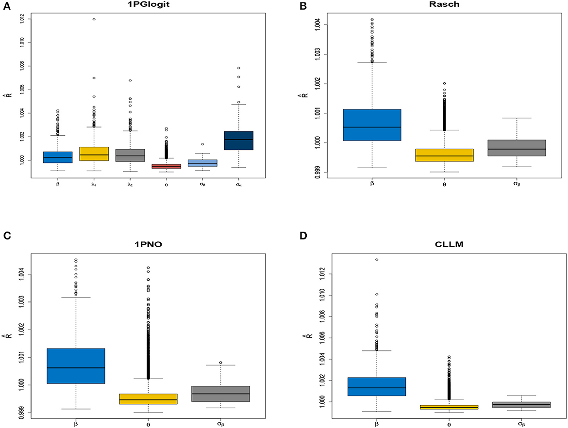
Figure 3. Boxplot of parameter $\widehat{R}$ in four models under N = 1, 000 and J = 20 conditions in simulation 1. (A) 1PGlogit model. (B) Rasch model. (C) 1PNO model. (D) CLLM.

FIGURE 4

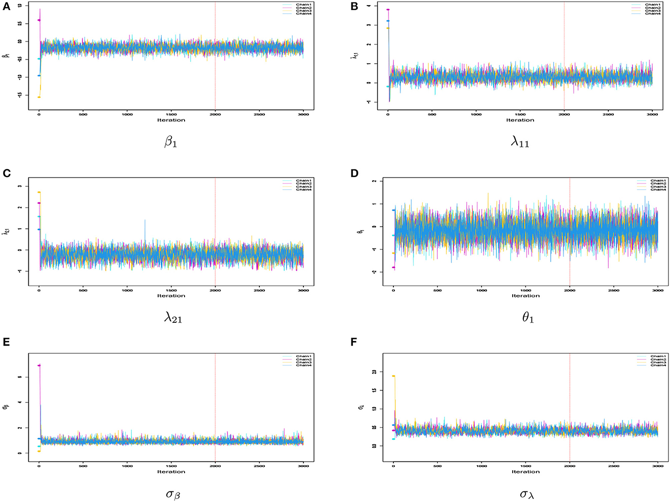
Figure 4. (A–F) Sampling trace plots of parameters β₁, λ₁₁, λ₂₁, θ₁, σ_β, and σ_λ in four Markov chains for 1PGlogit model under N = 1, 000 and J = 20 conditions in simulation 1.

4.1.3. Analysis of parameter estimation accuracy

In this study, we examine the accuracy of the estimation for the item parameters and latent trait parameters of each model. We computed the average bias, MSE, SE, and SD for each parameter, which are presented in Table 1. By examining the results in the table, we draw the following conclusions: First, the estimation appears unbiased, as reflected by the minimal and close-to-zero bias of all parameters. Second, our estimation exhibits large sample properties, meaning the precision of parameter estimation improves as the number of students increases for item parameters, and as the number of items increases for ability parameters. For instance, in the 1PGlogit model, as the sample size increases from N=1,000 to N=2,000, the MSE, SE, and SD of item parameters β, λ₁, λ₂ decrease. Similarly, when increasing from J=20 to J=40, the MSE, SE, and SD of θ decrease as well. Similar conclusions hold true in the Rasch, 1PNO, and CLLM models. Moreover, we observed that the estimation precision of latent trait parameters θ is not as robust as that of difficulty parameters β across all models. This can be attributed to the limited number of items (only 20 or 40 items). Specifically, in the 1PGlogit model, the estimation precision of λ is also poorer than that of β, and we speculate that this may be due to the interaction between λ and θ affecting the estimation precision.

TABLE 1

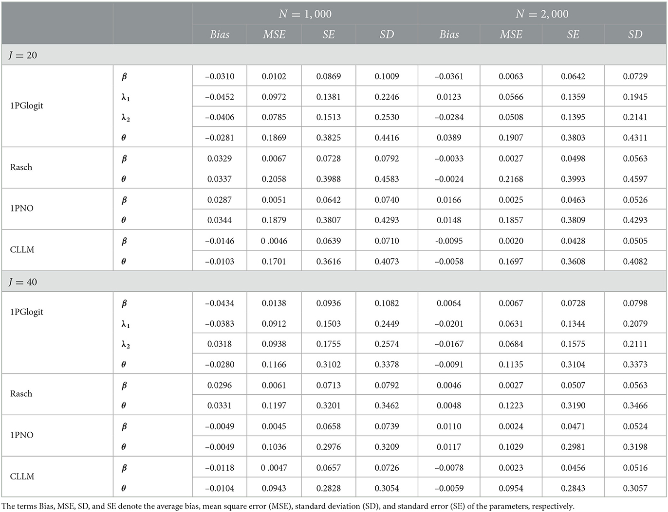
Table 1. Evaluating the accuracy of parameter estimation for various models and simulation conditions in simulation study 1.

4.2. Simulation 2

In this simulation study, our aim is to assess the model fit of traditional symmetric IRT models, asymmetric IRT model, and the Glogit IRT models under the framework of the one-parameter IRT.

We consider a sample size of N = 1, 000 individuals, with the test length fixed at 20. Item responses are generated within the framework of a one-parameter IRT model. We consider four item response models: (1) 1PGlogit(λ_1j, λ_2j), j = 1, 2, ..., J; (2) Rasch (1PGlogit(0, 0)); (3) 1PNO (1PGlogit(0.165, 0.165)); and (4) CLLM (1PGlogit(0.62, −0.037)). Therefore, we evaluate the model fitting in the following four cases.

• Case 1: True model: 1PGlogit(λ_1j, λ_2j) v.s. Fitted model: 1PGlogit(λ_1j, λ_2j), Rasch, 1PNO, and CLLM;

• Case 2: True model: Rasch v.s. Fitted model: 1PGlogit(λ_1j, λ_2j), Rasch, 1PNO, and CLLM;

• Case 3: True model: 1PNO v.s. Fitted model: 1PGlogit(λ_1j, λ_2j), Rasch, 1PNO, and CLLM;

• Case 4: True model: CLMM v.s. Fitted model: 1PGlogit(λ_1j, λ_2j), Rasch, 1PNO, and CLLM.

The true values and prior distributions for the parameters are specified in the same way as in simulation 1. To implement the MCMC sampling algorithm, chains of length 3,000 are chosen, with an initial burn-in period of 2,000. The results of the Bayesian model assessment, based on 50 replications, are shown in Table 2. It is worth noting that the reported results of DIC, LPML, WAIC, and LOO are based on the average of these 50 replications. The corresponding boxplots of the four Bayesian model assessment indexes is shown in Figure 5. Additionally, we have compiled the number of times each model was selected as the best or second-best model in Table 3.

TABLE 2

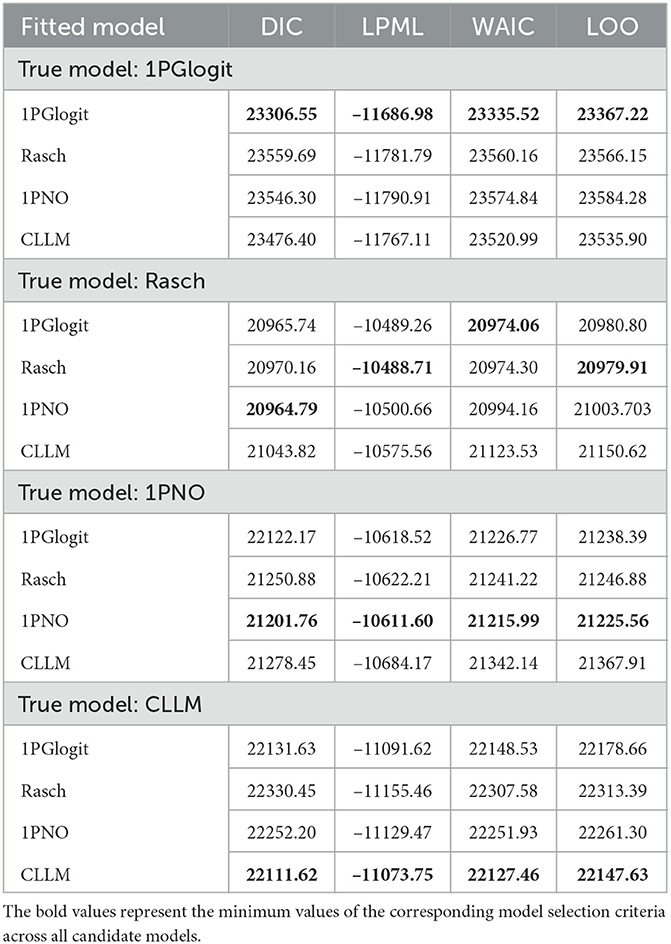
Table 2. Comparing the DIC, LPML, WAIC, and LOO values for 1PGlogit, Rasch, 1PNO, and CLLM models in simulation 2.

FIGURE 5

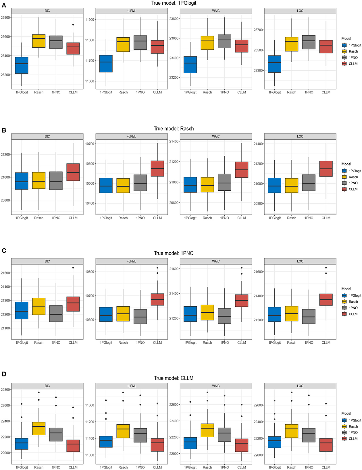
Figure 5. Boxplots of DIC, –LPML, WAIC, and LOO for 1PGlogit, Rasch, 1PNO, and CLLM models in simulation 2. (A) True model: 1PGlogit model. (B) True model: Rasch model. (C) True model: 1PNO model. (D) True model: CLLM.

TABLE 3

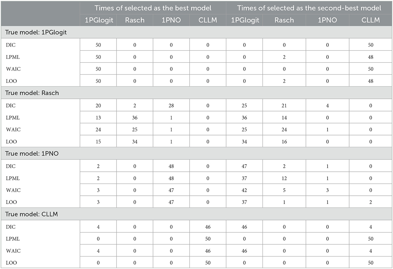
Table 3. Number of times selected as the best model and the second-best model based on DIC, LPML, WAIC, and LOO in simulation 2.

According to Tables 2, 3, when the true model is a 1PGlogit model, the 1PGlogit model is consistently chosen as the optimal model for data fitting based on the average values of the four model evaluation criteria, compared to the other three competing models. The second-best model is mostly the asymmetric CLLM, except for two instances where the Rasch model is selected for LPML and LOO criteria. When the true model is the CLLM model, the evaluation results are very similar to the case where the true model is the 1PGlogit model. With only a few exceptions, the CLLM model is chosen as the optimal model for almost all evaluation indicators, and the 1PGlogit model is chosen as the second-best model. Additionally, from Table 2 and Figure 5, we can observe that the fitting results of the 1PGlogit model are not significantly different from that of the CLLM model. In fact, 1PGlogit model has been selected four times as the best model using DIC and WAIC. However, the fitting results of the other two symmetric models, Rasch and 1PNO, are noticeably worse compared with that of the CLLM and 1PGlogit models. Interestingly, when the true model is the Rasch model, we observe that the fitting results of the 1PGlogit and 1PNO models are highly similar to those of the Rasch model. In terms of average DIC value, the 1PGlogit and 1PNO models even perform better and are often chosen as the best models. The Rasch model has only a very slight advantage over the 1PGlogit model in LPML and LOO, and in many cases, the 1PGlogit model is selected as the true model. The difference between 1PGlogit model and Rasch model, based on the four model evaluation criteria, is very small and less than 1. The fitting results of the 1PNO model are slightly worse than that of 1PGlogit and Rasch models based on LPML, WAIC, and LOO criteria, and the performance of the CLLM is the worst in all four evaluation criteria. In the case where the 1PNO model is the true model, we also observe that the performance of the CLLM is consistently the worst. While the 1PNO model slightly outperforms the 1PGlogit model across all model evaluation criteria, the 1PGlogit model still provides a good fit and has been selected as the best fitting model several times based on these model evaluation criteria.

Additionally, we chose the first item from four simulation conditions, respectively, and plotted their true ICCs against the four fitted ICCs for comparison in Figure 6. The true ICC is represented by the black line, while the red line illustrates the ICC fitted using 1PGlogit model. It can be noted that regardless of the true model type, our 1PGlogit model can provide an excellent fit, especially when the Rasch model and 1PNO model serve as the true model, the ICC fitted by 1PGlogit model almost coincides with the true ICC curve. In summary, 1PGlogit model proves to be a versatile generalized model that fits several widely used one-parameter IRT models effectively.

FIGURE 6

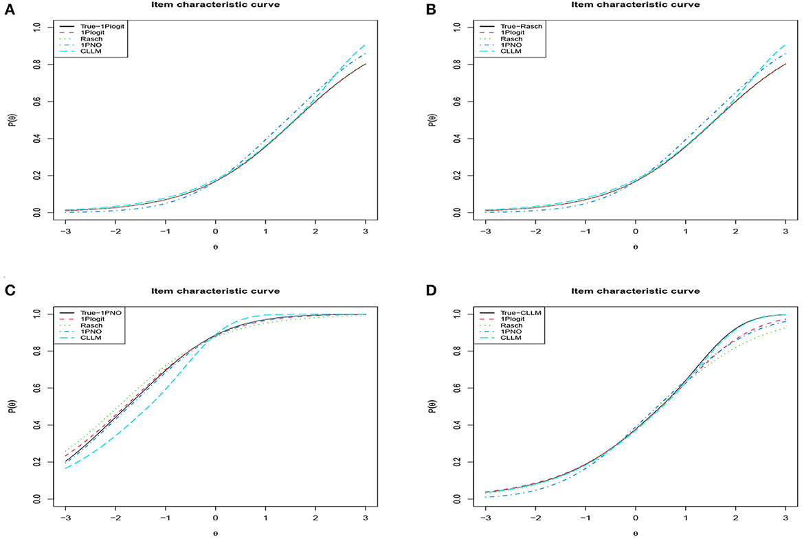
Figure 6. Analyzing the degree of fit for ICCs across different true models and fitting models in simulation 2. (A) True model: 1PGlogit with β₁ = −0.5734, λ₁₁ = 1, λ₂₁ = 1. (B) True model: Rasch (1PGlogit with β₁ = 1.5891, λ₁₁ = 0, λ₂₁ = 0). (C) True model: 1PNO (1PGlogit with β₁ = −1.7712, λ₁₁ = 0.165, λ₂₁ = 0.165). (D) True model: CLLM (1PGlogit with β₁ = 0.5036, λ₁₁ = 0.62, λ₂₁ = −0.037).

4.3. Simulation 3

In our previous discussion, we noted that the two shape parameters in the proposed 1PGlogit model can control whether the ICC has a heavy or light tail, playing a role similar to the lower asymptote parameter in the three-parameter IRT models, and the upper asymptote parameter in the more generalized four-parameter IRT models. In this simulation study, we focus on comparing the fit superiority of the 1PGlogit model with the traditional 3PL and 4PL models.

We consider a sample size of N = 1, 000 individuals, with the test length fixed at 20. Item responses are generated from the 3PL model and 4PL model. Therefore, we evaluate the model fitting in the following two cases.

• Case 1: True model: 3PL v.s. Fitted model: 1PGlogit(λ_1j, λ_2j), Rasch, 1PNO, CLLM, and 3PL;

• Case 2: True model: 4PL v.s. Fitted model: 1PGlogit(λ_1j, λ_2j), Rasch, 1PNO, and CLLM, and 4PL.

The true values of parameters in the 3PL and 4PL models are generated as follows: α_j ~ U(0.5, 2), β_j ~ N(0, 1), c_j ~ Beta(5, 17) and d_j ~ Beta(17, 5) (d_j = 1 for 3PL model). The prior distribution of parameters in the 1PGlogit model, Rasch model, 1PNO model, and CLLM are generated the same as in simulation 1. Moreover, we wish to clarify the prior distributions setting for the parameters in the 3PL/4PL models: logα_j ~ N(0, 1), ${\beta }_j~\mathrm{\text{N}}(0,{\sigma }_{\beta }^2)$, c_j ~ U(0, 0.5), d_j ~ U(0, 0.5) (in 4PL model), and σ_β ~ Cauchy(0, 5). To implement the MCMC sampling algorithm, chains of length 5,000 are chosen, with an initial burn-in period of 4,000.

In Table 4, we present the DIC, LPML, WAIC, and LOO values for each model. Figure 7 depicts the boxplots of these four model selection criteria across 50 replications. Additionally, Table 5 summarizes the instances where each model was selected as the best or second best fitting model across the 50 replications. The results indicate that when the true model is the 3PL model, the average values of –LPML, WAIC, and LOO for the 3PL model are the lowest among all models under consideration. In all 50 replications, these evaluation criteria identify the true 3PL model as the best model. For the second-best model selection, apart from LOO (which chose the Rasch model once), all other criteria consistently select the 1PGlogit model. Although the average DIC value for the 3PL model is the lowest, it differs from the other three criteria. In 12 out of 50 replications, the 1PGlogit model is selected as the best model, and in 38 replications, it's chosen as the second-best model. These findings suggest that our flexible 1PGlogit model can effectively fit the 3PL model. Considering the values of various model selection criteria and the boxplot results, the fitting performance of the 1PGlogit model is significantly superior to other one-parameter models. To further illustrate this, we plotted the ICC of the first item for the true 3PL model, as well as ICC curves fitted by the five different models in Figure 8. The plots reveal that, aside from the fitted 3PL model, our 1PGlogit model shows the best fit with the true ICC, regardless of item difficulty. In the 3PL model, the assumed guessing behavior causes the lower asymptote of its ICC to be above zero. Our 1PGlogit model can account for this phenomenon through the parameter λ, suggesting that our model can also interpret the assumed guessing behavior inherent in the 3PL model.

TABLE 4

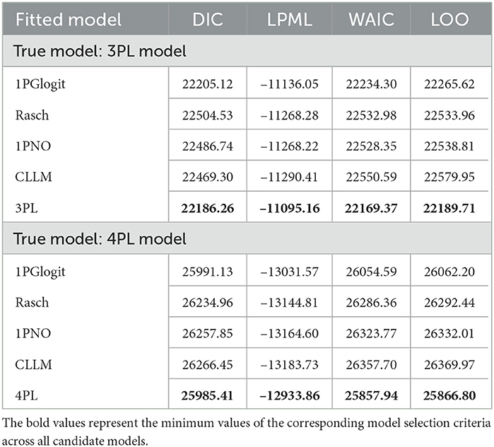
Table 4. Comparing the DIC, LPML, WAIC, and LOO values for 1PGlogit, Rasch, 1PNO, CLLM, 3PL, and 4PL models in simulation 3.

FIGURE 7

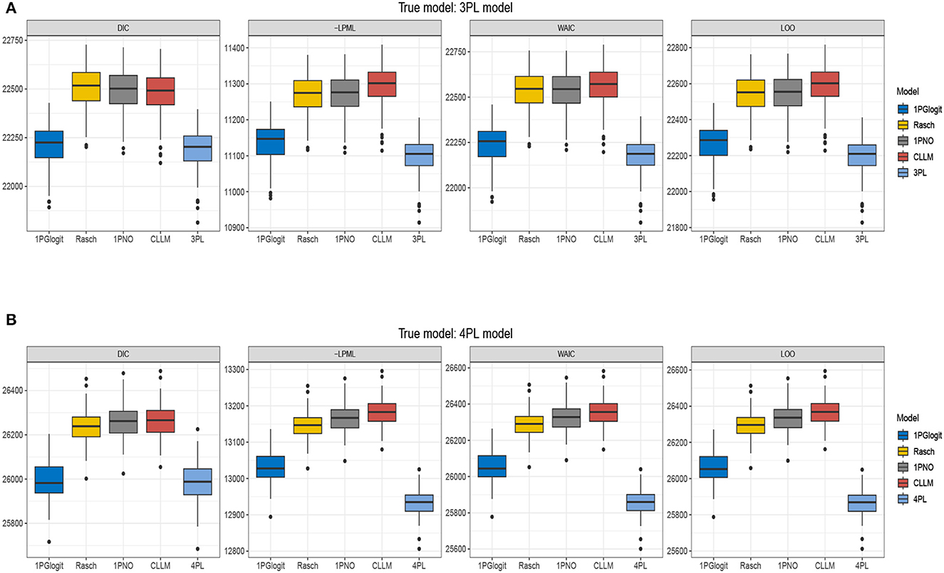
Figure 7. Boxplots of DIC, –LPML, WAIC, and LOO for 1PGlogit, Rasch, 1PNO, CLLM, 3PL, and 4PL models in simulation 3. (A) True model: 3PL model. (B) True model: 4PL model.

TABLE 5

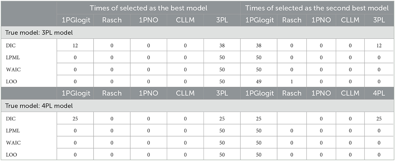
Table 5. Number of selected times as the best-model and the second-best model based on DIC, LPML, WAIC, and LOO in Simulation 3.

FIGURE 8

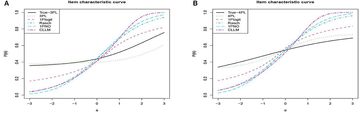
Figure 8. Analyzing the degree of fit for ICCs across different true models and fitting models in simulation 3. (A) True model: 3PL model with α₁ = 0.7766, β₁ = 2.3315, c₁ = 0.3470. (B) True model: 4PL model with α₁ = 0.5167, β₁ = −1.0322, c₁ = 0.1894, d₁ = 0.7518.

Secondly, when the true model is the 4PL model, the results are nearly identical to those under the 3PL model. The 4PL model performs the best based on LPML, WAIC, and LOO, and is selected as the optimal model in all 50 repetitions. The second-best model is consistently the 1PGlogit model. In terms of DIC value, the average for the 4PL model is the lowest, but in 25 out of 50 repetitions, the 1PGlogit model is chosen as the best. As illustrated by the boxplot in Figure 7, the model selection criteria of the 1PGlogit model are significantly lower than those of the other one-parameter models. Figure 8 displays the ICCs of the first item. Aside from the 4PL model, the ICC of the 1PGlogit model demonstrates the best fitting performance, suggesting that this flexible 1PGlogit model provides a well-fitted representation of the guessing behavior and slipping behavior assumed in the 4PL model, which affects the lower and upper asymptotes.

In summary, the 1PGlogit model demonstrates superior fitting performance for asymmetric models compared to other one-parameter models. This model enhances flexibility by adjusting the parameter λ to fit the upper and lower asymptotes. However, we observed that DIC sometimes failed to identify the true model in this simulation, as was also the case when Rasch was the true model in Simulation 2. According to Luo and Al-Harbi (2016), within the dichotomous IRT framework, the performances of WAIC and LOO surpass that of DIC. Therefore, in light of the findings of this paper, we recommend giving greater consideration to LPML, WAIC, and LOO criteria when selecting models.

5. Real data

For this example, we use the 2015 computer-based PISA science data. Out of all the countries that took part in the computer-based science assessment, we selected data from the United States of America (USA). The initial sample consisted of 685 students, but 76 students were excluded due to Not Reached (original code 6) or No Response (original code 9) outcomes. These Not Reached and No Response results were treated as missing data. Therefore, the final sample size stands at 609 students, for whom the response data is available. The 11 items were scored on a dichotomous scale. We utilize six different models to fit the PISA dataset. This includes two symmetric models, namely the Rasch and the 1PNO models, in conjunction with three asymmetric models: the CLLM, the 3PL model, the 4PL model, and our generalized logistic model, known as the 1PGlogit model. During the process of estimation, we employ the same prior probabilities for the unknown parameters as used in simulations 2 and 3. Throughout all Bayesian computations, we generate 5,000 MCMC samples after a burn-in period of 4,000 iterations for each model to compute all the posterior estimates. The convergence of the chains is assured by evaluating the PSRF values ($\widehat{R}$). For each model, the PSRF values of all parameters, both item and person, are observed to be under 1.1.

First, we depicted the frequency distribution histogram of the estimated ability parameter θ values across different models in Figure 9, and fitted their respective distribution curves. From this, it is apparent that the distributions of the estimated ability parameters remain largely consistent across the varied models. Upon examining the fitted distributions of the estimated θ, it can be observed that the ability distribution under the 1PGlogit model is closest to a normal distribution. The θ distributions under the Rasch and 1PNO models are notably similar, while the θ distributions under the 3PL model are more analogous to those of the 4PL model. Next, we provide detailed results of the Bayesian model assessment for the PISA dataset in Table 6. All these criteria indicate that the 1PGlogit model fits the data best among the six models. The second-best fitting model tends to be either the 3PL model or the 4PL model, both of which demonstrate similar fitting effects, while the three one-parameter IRT models show a notably inferior fit compared to the others. Hence, we surmise that the data shows a preference for flexible asymmetrical models. Based on the results of the model assessment, we will proceed with the best fitting 1PGlogit model for the analysis of the PISA data. In Table 7, we provide the estimated values of parameters in the 1PGlogit model, including the SD, 95% highest posterior density interval (HPDI), and $\widehat{R}$ for each parameter. It is evident from the $\widehat{R}$ values that the Markov chain has achieved convergence. Examining the estimated parameter values, we note firstly that item 6 is the most difficult, with β₆ = 2.4805, while item 11 is the easiest, with β₁₁ = −2.5073. Moreover, for the parameter λ₁, the values are mostly small, except for item 5 which exceeds 1, suggesting that the tail of this item's ICC approaches the upper asymptote more quickly. Conversely, the estimated values for λ₂ are generally larger and positive, such as for item 10, which exceeds 1, indicating a rapid approach to the lower asymptote for the tail of its ICC. Lastly, we have plotted the ICCs for all the items in Figure 10. From Figure 10, it can be seen that for item 2, there appears to be some guessing behavior among low ability students, as they have a certain probability of answering the item correctly even with very low ability. Conversely, high ability students may exhibit slipping behavior, as even with relatively high ability, their probability of answering correctly is only around 90%. In contrast, for item 5, students with ability values below 2 have virtually no chance of answering correctly, while those with ability values exceeding 1.5 have almost no chance of answering incorrectly. In essence, the 1PGlogit model can deliver robust data fitting and outstanding interpretability.

FIGURE 9

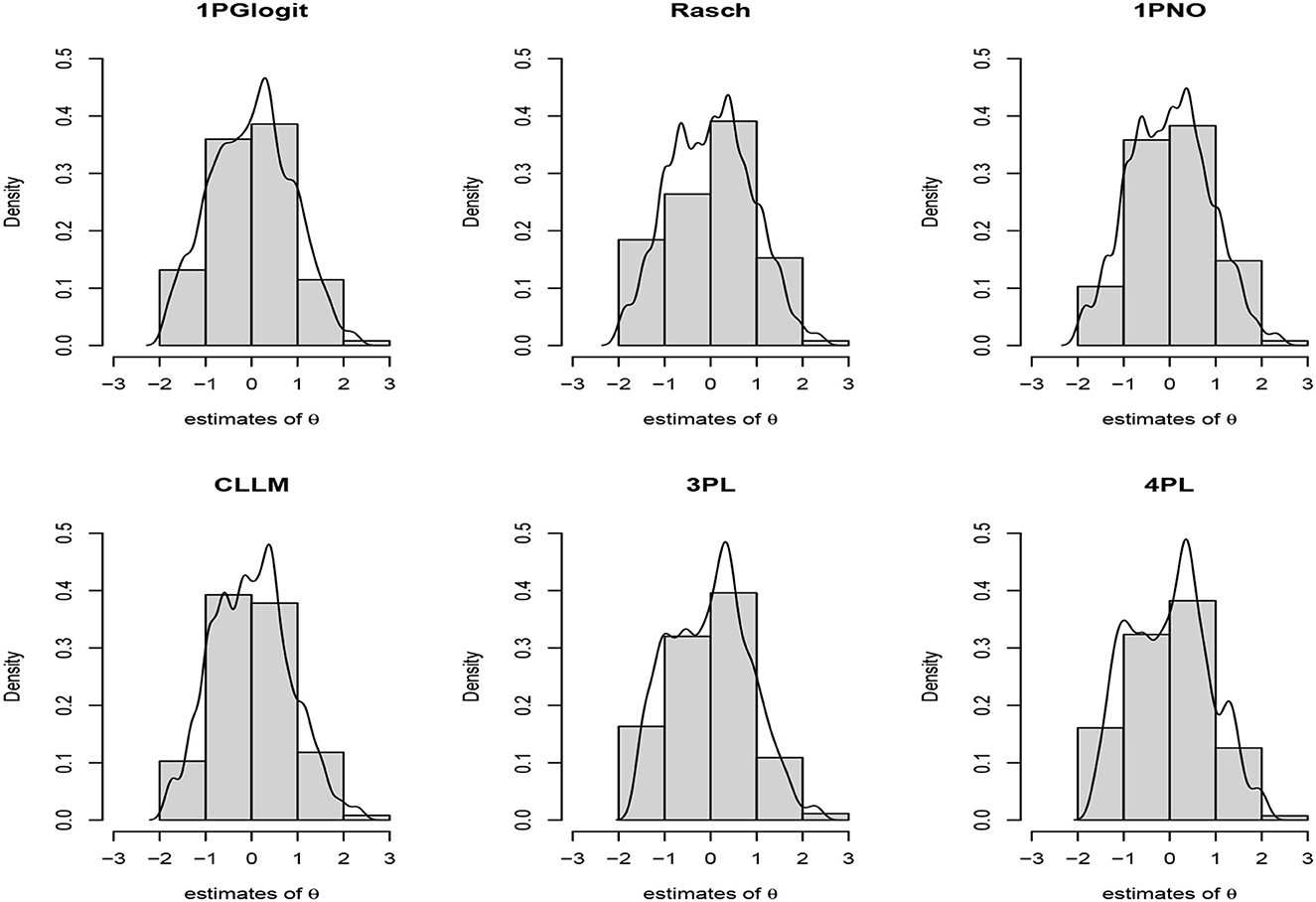
Figure 9. Item characteristic curve (ICC) of all items based on 1PGlogit model for the real data.

TABLE 6

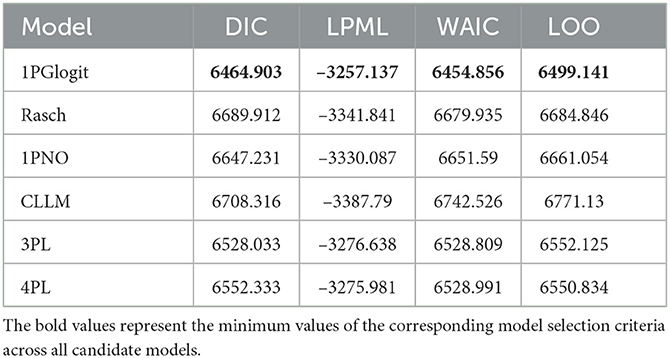
Table 6. Values of DIC, LPML, WAIC, and LOO for 1PGlogit, Rasch, 1PNO, CLLM, 3PL, and 4PL models for the real data.

TABLE 7

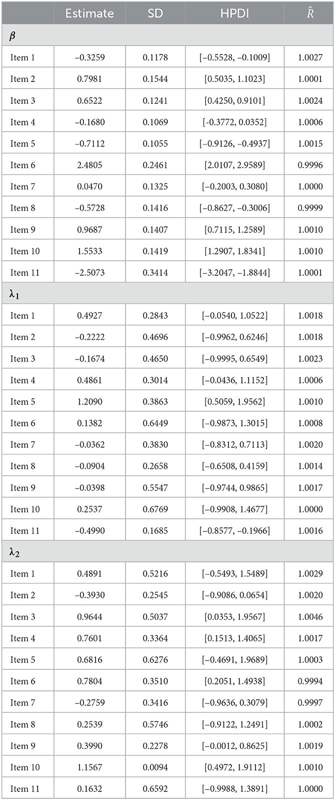
Table 7. Parameter estimates for all items based on the 1PGlogit model in real data.

FIGURE 10

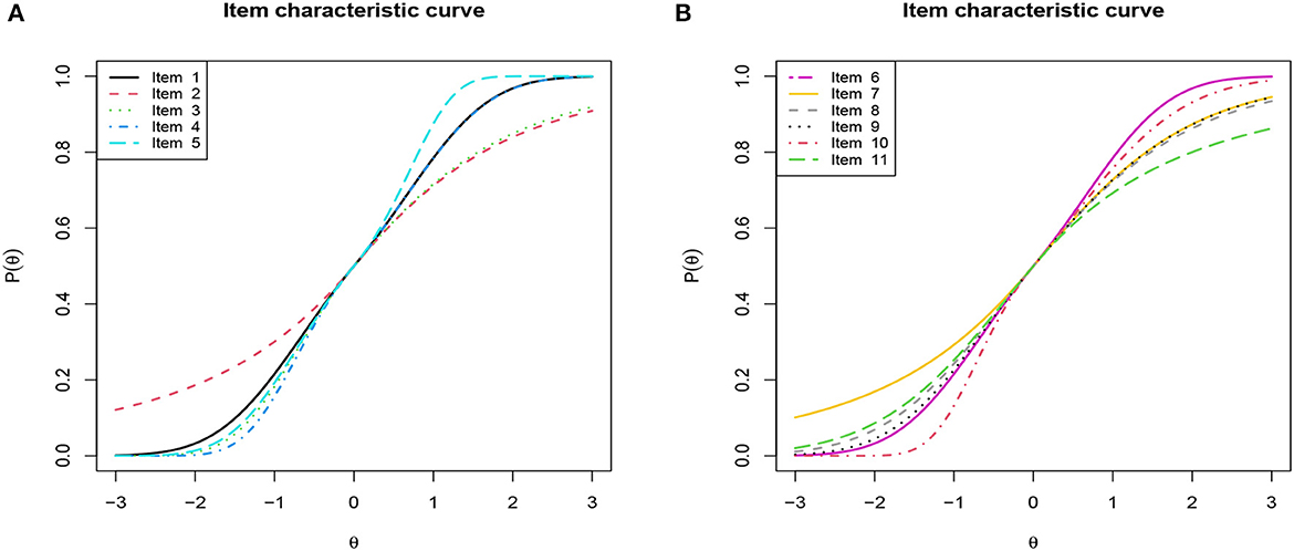
Figure 10. Item characteristic curve (ICC) of all items based on 1PGlogit model for the real data. (A) ICC of Item 1–5. (B) ICC of Item 6–11.

6. Discussion

This paper discusses a generalized one-parameter IRT model, the 1PGlogit model, which can encompass commonly-used IRT models such as the Rasch, 1PNO, and the recently proposed CLLM as its submodels. Owing to its adjustable parameter λ, it exhibits high flexibility, which enables control over the rate at which it approaches the upper and lower asymptotes of the ICC. In this paper, we first examine the accuracy of the model in parameter recovery using the Stan program. Subsequently, we investigate its performance in fitting data generated by other one-parameter IRT models. Finally, we delve deeper into its effectiveness in fitting asymmetric 3PL and 4PL models.

From the simulation results, we can draw the following conclusions. Firstly, the estimates generated by Stan are consistent with the large sample properties and exhibit excellent parameter recovery accuracy. The difficulty parameter demonstrates the highest estimation precision, followed by λ and θ. Secondly, the 1PGlogit model showcases commendable fitting performance for data generated by its various submodels. It ranks as the best model in terms of fitting performance, with the exception of the true model. Finally, the 1PGlogit model presents an outstanding fit for data generated by the asymmetric 3PL and 4PL models, markedly superior to other one-parameter IRT models. The 1PGlogit model can more accurately recover the shape of the ICC of the 3PL/4PL model.

In summary, the 1PGlogit model is a highly flexible and generalized model that encompasses Rasch, 1PNO, and CLLM as its submodels. Its parameter λ adjusts the speed at which the ICC curve approaches the upper and lower asymptotes. A larger λ₁ results in a quicker approach to the upper asymptote, and a larger λ₂ results in a swifter approach to the lower asymptote. As such, the 1PGlogit model can effectively accommodate the assumptions of guessing and slipping behavior in the 3PL and 4PL models, which would otherwise cause the upper and lower asymptotes to diverge from 1 and 0, respectively. However, the 1PGlogit model also has its limitations. Firstly, the constraint that its parameter λ must be greater than -1 may inhibit the model's ability to depict behaviors on the ICC where the asymptotes significantly diverge from 1 and 0. Secondly, although the 1PGlogit model is a generalized model that includes other one-parameter IRT models, the introduction of the new parameter λ adds complexity to the model, and the estimation accuracy of 1PGlogit is slightly lower than that of other one-parameter models. Moreover, the introduction of λ may also introduce some identifiability issues to the model, where λ and θ might mutually influence each other.

In conclusion, we would like to propose some directions for future work. The 1PGlogit model is a flexible and generalized model, and this paper merely provides an initial exploration of its advantages in fitting various types of data. We believe there is significant potential for its further development and application, such as extending the 1PGlogit model to higher-order IRT models, graded response models, multilevel IRT models, and longitudinal IRT models, among others. Therefore, in our future research, we will dedicate ourselves to the advancement and application of the 1PGlogit model in these proposed areas. Moreover, a wealth of scholarly work has been dedicated to formulating link functions for binary and ordinal response data. Notable contributions in this field have been made by Aranda-Ordaz (1981), Guerrero and Johnson (1982), Stukel (1988), Kim et al. (2008), Wang and Dey (2010), and Jiang et al. (2014), among others. It is worth exploring whether these existing link functions can be directly applied to the field of IRT. We intend to investigate this possibility in our future work.

Data availability statement

Publicly available datasets were analyzed in this study. This data can be found at: https://www.oecd.org/pisa/data/.

Author contributions

XW and JZ completed the writing of this article. XW, JZ, and JL completed the article revisions. JL provided original thoughts. JZ, JL, GC, and NS provided key technical support. All authors contributed to the article and approved the submitted version.

Funding

This work was supported by Jilin Province Education Science 14th Five-Year Plan 2022 Annual General Topic + Dynamic Education Quality Monitoring and Evaluation Research Supported by Data - Taking Jilin Province Mathematics Academic Ability Growth Assessment as an Example + Project Approval Number GH22415 and Guangdong Basic and Applied Basic Research Foundation (No. 2022A1515011899).

Conflict of interest

The authors declare that the research was conducted in the absence of any commercial or financial relationships that could be construed as a potential conflict of interest.

Publisher's note

All claims expressed in this article are solely those of the authors and do not necessarily represent those of their affiliated organizations, or those of the publisher, the editors and the reviewers. Any product that may be evaluated in this article, or claim that may be made by its manufacturer, is not guaranteed or endorsed by the publisher.

Supplementary material

The Supplementary Material for this article can be found online at: https://www.frontiersin.org/articles/10.3389/fpsyg.2023.1248454/full#supplementary-material

References

Aranda-Ordaz, F. J. (1981). On two families of transformations to additivity for binary response data. Biometrika 68, 357–363. doi: 10.1093/biomet/68.2.357

CrossRef Full Text | Google Scholar

Arenson, E. A., and Karabatsos, G. (2018). A Bayesian beta-mixture model for nonparametric IRT (BBM-IRT). J. Modern Appl. Stat. Methods 17, 1–18. doi: 10.22237/jmasm/1531318047

CrossRef Full Text | Google Scholar

Baker, F. B., and Kim, S. H. (2004). Item Response Theory: Parameter Estimation Techniques, 2nd Edn. CRC Press. doi: 10.1201/9781482276725

CrossRef Full Text | Google Scholar

Bechtel, G. G. (1985). Generalizing the Rasch model for consumer rating scales. Market. Sci. 4, 62–73. doi: 10.1287/mksc.4.1.62

PubMed Abstract | CrossRef Full Text | Google Scholar

Bezruczko, N. (2005). Rasch Measurement in Health Sciences. Maple Grove, MN: Jam Press.

Google Scholar

Bolfarine, H., and Bazan, J. L. (2010). Bayesian estimation of the logistic positive exponent IRT model. J. Educ. Behav. Stat. 35, 693–713. doi: 10.3102/1076998610375834

CrossRef Full Text | Google Scholar

Brooks, S. P., and Gelman, A. (1998). Alternative methods for monitoring convergence of iterative simulations. J. Comput. Graph. Stat. 7, 434–455. doi: 10.1080/10618600.1998.10474787

CrossRef Full Text | Google Scholar

Chen, M. H., Dey, D. K., and Shao, Q. M. (1999). A new skewed link model for dichotomous quantal response data. J. Am. Stat. Assoc. 94, 1172–1186. doi: 10.1080/01621459.1999.10473872

CrossRef Full Text | Google Scholar

Chen, M. H., Dey, D. K., and Wu, Y. (2002). On robustness of choice of links in binomial regression. Calcutta Stat. Assoc. Bull. 53, 145–164. doi: 10.1177/0008068320020113

CrossRef Full Text | Google Scholar

Duncan, K., and MacEachern, S. (2008). Nonparametric Bayesian modelling for item response. Stat. Modell. 8, 41–66. doi: 10.1177/1471082X0700800104

CrossRef Full Text | Google Scholar

Embretson, S. E., and Reise, S. P. (2000). Item Response Theory for Psychologists. Lawrence Erlbaum Associates.

Google Scholar

Ferguson, G. A. (1942). Item selection by the constant process. Psychometrika 7, 19–29. doi: 10.1007/BF02288601

CrossRef Full Text | Google Scholar

Geisser, S., and Eddy, W. F. (1979). A predictive approach to model selection. J. Am. Statist. Assoc. 74, 153–160. doi: 10.1080/01621459.1979.10481632

CrossRef Full Text | Google Scholar

Geman, S., and Geman, D. (1984). Stochastic relaxation, Gibbs distributions, and the Bayesian restoration. IEEE Trans. Pattern Anal. Mach. Intell. 6, 721–741.

PubMed Abstract | Google Scholar

Goldstein, H. (1980). Dimensionality and the fitting of unidimensional item response models to multidimensional data. Appl. Psychol. Meas. 4, 355–365.

PubMed Abstract | Google Scholar

Guerrero, V. M., and Johnson, R. A. (1982). Use of the Box-Cox transformation with binary response models. Biometrika 69, 309–314. doi: 10.1093/biomet/69.2.309

CrossRef Full Text | Google Scholar

Hoffman, M. D., and Gelman, A. (2014). The No-U-Turn sampler: adaptively setting path lengths in Hamiltonian Monte Carlo. J. Mach. Learn. Res. 15, 1593–1623. Available online at: https://jmlr.org/papers/v15/hoffman14a.html

Google Scholar

Ibrahim, J. G., Chen, M. H., and Sinha, D. (2001). Bayesian Survival Analysis. New York, NY: Springer.

Google Scholar

Jiang, X., Dey, D. K., Prunier, R., Wilson, A. M., and Holsinger, K. E. (2014). A new class of flexible link functions with application to species co-occurrence in Cape floristic region. Ann. Appl. Stat. 7, 2180–2204 doi: 10.1214/13-AOAS663

CrossRef Full Text | Google Scholar

Karabatsos, G. (2016). “Bayesian nonparametric IRT,” in Handbook of Item Response Theory, Vol. 1, ed W. J. van der Linden (Boca Raton, FL: Chapman and Hall/CRC), 323–336.

Google Scholar

Kim, S., Chen, M.-H., and Dey, D. K. (2008). Flexible generalized t-link models for binary response data. Biometrika 95, 93–106. doi: 10.1093/biomet/asm079

CrossRef Full Text | Google Scholar

Lawley, D. N. (1943). On problems connected with item selection and test construction. Proc. R. Soc. Edinburgh 61, 273–287. doi: 10.1017/S0080454100006282

PubMed Abstract | CrossRef Full Text | Google Scholar

Lawley, D. N. (1944). The factorial invariance of multiple item tests. Proc. R. Soc. Edinburgh, 62-A, 74–82. doi: 10.1017/S0080454100006440

CrossRef Full Text | Google Scholar

Lord, F. M. (1952). A theory of test scores. Psychometr. Monogr. 7, 1–100.

Google Scholar

Lord, F. M. (1953). An application of confidence intervals and of maximum likelihood to the estimation of an examinee's ability. Psychometrika 18, 57–75. doi: 10.1007/BF02289028

CrossRef Full Text | Google Scholar

Lord, F. M. (1980). Applications of Item Response Theory to Practical Testing Problems. Hillsdale, NJ: Lawrence Erlbaum Associates.

Google Scholar

Lord, F. M., and Novick, M. R. (1968). Statistical Theories of Mental Test Scores. Menlo Park, CA: Addison-Wesley.

Google Scholar

Lucke, J. F. (2014). “Positive trait item response models,” in New Developments in Quantitative Psychology: Presentations from the 77th Annual Psychometric Society Meeting, eds R. E. Millsap, L. A. van der Ark, D. M. Bolt, and C. M. Woods (New York, NY: Routledge), 199–213. doi: 10.1007/978-1-4614-9348-8_13

CrossRef Full Text | Google Scholar

Lunn, D. J., Thomas, A., Best, N., and Spiegelhalter, D. (2000). WinBUGS-a Bayesian modelling framework: concepts, structure, and extensibility. Stat. Comput. 10, 325–337. doi: 10.1023/A:1008929526011

CrossRef Full Text | Google Scholar

Luo, Y., and Al-Harbi, K. (2016). “Performances of LOO and WAIC as IRT model selection methods,” in Paper presented at the International Meeting of Psychometric Society (Ashville, NC).

Google Scholar

Luo, Y., and Jiao, H. (2018). Using the Stan program for Bayesian item response theory. Educ. Psychol. Meas. 78, 384–408. doi: 10.1177/0013164417693666

PubMed Abstract | CrossRef Full Text | Google Scholar

Luzardo, M., and Rodriguez, P. (2015). “A nonparametric estimator of a monotone item characteristic curve,” in Quantitative Psychology Research, eds L. A. van der Ark, D. Bolt, W. C. Wang, A. Douglas, and S. M. Chow (Cham: Springer International Publishing), 99–108. doi: 10.1007/978-3-319-19977-1_8

CrossRef Full Text | Google Scholar

Magnus, B. E., and Liu, Y. (2018). A zero-inflated Box-Cox normal unipolar item response model for measuring constructs of psychopathology. Appl. Psychol. Meas. 42, 571–589. doi: 10.1177/0146621618758291

PubMed Abstract | CrossRef Full Text | Google Scholar

Metropolis, N., Rosenbluth, A. W., Rosenbluth, M. N., Teller, A. H., and Teller, E. (1953). Equation of state calculations by fast computing machines. J. Chem. Phys. 21, 1087–1092. doi: 10.1063/1.1699114

CrossRef Full Text | Google Scholar

Moral, F. J., and Rebollo, F. J. (2017). Characterization of soil fertility using the Rasch model. J. Soil Sci. Plant Nutr. doi: 10.4067/S0718-95162017005000035

PubMed Abstract | CrossRef Full Text | Google Scholar

Mosier, C. L. (1940). Psychophysics and mental test theory: fundamental postulates and elementary theorems. Psychol. Rev. 47, 355–366. doi: 10.1037/h0059934

CrossRef Full Text | Google Scholar

Mosier, C. L. (1941). Psychophysics and mental test theory. II. The constant process. Psychol. Rev. 48, 235–249. doi: 10.1037/h0055909

CrossRef Full Text | Google Scholar

Neal, R. M. (2011). “MCMC using Hamiltonian dynamics,” in Handbook of Markov Chain Monte Carlo, Vol. 2, ed S. Brooks (Boca Raton, FL: CRC Press/Taylorand Francis), 113–162. doi: 10.1201/b10905-6

CrossRef Full Text | Google Scholar

Plummer, M. (2003). “JAGS: a program for analysis of Bayesian graphical models using Gibbs sampling,” in Proceedings of the 3rd International Workshop on Distributed Statistical Computing (DSC 2003) (Vienna), 20–22.

Google Scholar

Qin, L. (1998). Nonparametric Bayesian models for item response data (Unpublished doctoral dissertation). The Ohio State University, Columbus, OH, United States.

Google Scholar

R Core Team (2019). R: A Language and Environment for Statistical Computing. R Foundation for Statistical Computing, Vienna.

Google Scholar

Rasch, G. (1960). Probabilistic Model for Some Intelligence and Achievement Tests. Copenhagen: Danish Institute for Educational Research.

Google Scholar

Richardson, M. W. (1936). The relation between the difficulty and the differential validity of a test. Psychometrika 1, 33–49. doi: 10.1007/BF02288003

CrossRef Full Text | Google Scholar

Samejima, F. (1997). “Ability estimates that order individuals with consistent philosophies,” in Paper presented at the 1997 Meeting of the American Educational Research Association (Chicago, IL).

Google Scholar

Samejima, F. (1999). “Usefulness of the logistic positive exponent family of models in educational measurement,” in Paper presented at the 1999 Meeting of the American Educational Research Association (Montreal, QC).

Google Scholar

Samejima, F. (2000). Logistic positive exponent family of models: virtue of asymmetric item characteristics curves. Psychometrika 65, 319–335. doi: 10.1007/BF02296149

CrossRef Full Text | Google Scholar

Shim, H., Bonifay, W., and Wiedermann, W. (2022). Parsimonious asymmetric item response theory modeling with the complementary log-log link. Behav. Res. Methods 55, 200–219. doi: 10.3758/s13428-022-01824-5

PubMed Abstract | CrossRef Full Text | Google Scholar

Spiegelhalter, D. J., Best, N. G., Carlin, B. P., and Van Der Linde, A. (2002). Bayesian measures of model complexity and fit. J. R. Stat. Soc. Ser. B Stat. Methodol. 64, 583–639. doi: 10.1111/1467-9868.00353

CrossRef Full Text | Google Scholar

Spiegelhalter, D. J., Thomas, A., Best, N. G., and Lunn, D. (2010). OpenBUGS Version 3.1.1 User Manual.

Google Scholar

Stan Development Team (2019). Stan Modeling Language: User's Guide and Reference Manual.

Google Scholar

Stukel, T. A. (1988). Generalized logistic models. J. Am. Stat. Assoc. 83, 426–431. doi: 10.1080/01621459.1988.10478613

CrossRef Full Text | Google Scholar

Tucker, L. R. (1946). Maximum validity of a test with equivalent items. Psychometrika 11, 1–13. doi: 10.1007/BF02288894

PubMed Abstract | CrossRef Full Text | Google Scholar

van der Linden, W. J., and Hambleton, R. K. (1997). Handbook of Modern Item Response Theory. New York, NY: Springer. doi: 10.1007/978-1-4757-2691-6

PubMed Abstract | CrossRef Full Text | Google Scholar

Vehtari, A., Gelman, A., and Gabry, J. (2017). Practical Bayesian model evaluation using leave-one-out cross-validation and WAIC. Stat. Comput. 27, 1413–1432. doi: 10.1007/s11222-016-9696-4

CrossRef Full Text | Google Scholar

Wang, X., and Dey, D. K. (2010). Generalized extreme value regression for binary response data: An application to B2B electronic payments system adoption. Ann. Appl. Stat. 4, 2000–2023. doi: 10.1214/10-AOAS354

CrossRef Full Text | Google Scholar

Watanabe, S., and Opper, M. (2010). Asymptotic equivalence of bayes cross validation and widely applicable information criterion in singular learning theory. J. Mach. Learn. Res. 11, 3571–3594. Available online at: https://www.jmlr.org/papers/volume11/watanabe10a/watanabe10a.pdf

Google Scholar

Wright, B. D. (1977). Solving measurement problems with the Rasch mode. J. Educ. Measure. 14, 97–116. doi: 10.1111/j.1745-3984.1977.tb00031.x

PubMed Abstract | CrossRef Full Text | Google Scholar

Zhang, J., Zhang, Y. Y., Tao, J., and Chen, M. H. (2022). Bayesian item response theory models with flexible generalized logit links. Appl. Psychol. Meas. 46, 382–405. doi: 10.1177/01466216221089343

PubMed Abstract | CrossRef Full Text | Google Scholar