
- Department of Vision Sciences, University of Alabama at Birmingham, Birmingham, AL, USA
Many previous studies have used the presentation of multiple stimuli in the receptive fields (RFs) of visual cortical neurons to explore how neurons might operate on multiple inputs. Most of these experiments have used two fixed stimulus locations within the RF of each neuron. Here the effects of using different positions within the RF of a neuron were explored. The stimuli were presented singly at one of six locations, and also at 15 pair-wise combinations, for 24 V2 cortical neurons in two macaque monkeys. There was considerable variability in how pairs of stimuli interacted within the receptive field of any given neuron: changing the position of the stimuli could result in enhancement, winner-take-all, or suppression relative to the strongest response to a stimulus presented by itself. Across the population of neurons there was no correlation between response strength and response latency. However, for many stimulus pairs the response latency was tightly locked to the shortest response latency of any single stimulus presented by itself independent of changes in response magnitude. In other words, a stimulus that by itself elicited a relatively long latency response, would often affect the magnitude of the response to a pair of stimuli, but not change the latency. These results may provide constraints on the development of models of cortical information processing.
Introduction
The cerebral neocortex is notable for the richness of inputs to each area and also to each neuron. How a cortical neuron operates on these multiple inputs to produce an output is a major ongoing area of research. Unlike other areas of the brain, such as the hippocampus, the anatomy of the cerebral neocortex is such that an experimenter cannot easily control the direct inputs to a single neuron. Many experiments have used the presentation of two separate visual stimuli in the receptive field (RF) of a visual cortical neuron as a surrogate for stimulating two inputs. This is a powerful technique, and much has been learned using it, especially as regards the effect of changes in selective attention.
In general, studies using two stimuli in the RF of visual cortical neurons in a wide array of different areas have each found a diversity of results between different neurons. Some studies have found that the general tendency is for the response to two stimuli to be near the weighted average of the responses to each stimulus presented separately (Moran and Desimone, 1985; Luck et al., 1997; Reynolds et al., 1999; Reynolds and Desimone, 2003; Zoccolan et al., 2005). Other studies have found that it was more common for the response to two stimuli to be similar in magnitude to the larger of the responses to the two stimuli presented separately, a winner-take-all or “MAX” result, at least for high-contrast stimuli (Sato, 1989; Heuer and Britten, 2002; Rolls et al., 2003; Lampl et al., 2004; Finn and Ferster, 2007; Oleksiak et al., 2011). In an attempt to limit the possible interactions at earlier processing stages, studies in this laboratory used two stimuli that were presented as far apart from each other as possible while still remaining within the RF (Gawne and Martin, 2002a; Gawne, 2008), and found a strong tendency for a MAX operation. It has also been proposed that both weighted averaging and MAX are too simplistic and that models of summation within a RF with more free parameters are required (Ghose and Maunsell, 2008). It must also be pointed out that previous studies show a wide diversity of selection criteria for choosing the stimuli, which could account for the diversity of results between different studies. However, this still does not explain the diversity of results seen within each study.
Most of these previous studies used only two fixed stimulus locations within the RF of each neuron. Given that these studies typically find a wide range of behaviors between neurons, this raises the question as to whether this response diversity is due to different neurons implementing different operations which they each apply uniformly to all stimuli, or if different positioning of stimuli within the RF could lead to apparently different combinatorial rules for a single neuron. To address this issue the responses of 24 single primate V2 neurons to stimuli presented at six fixed locations within the RF and to all 15 pair-wise combinations were recorded. The results indicate that, for closely apposed stimuli within the RF, different configurations of stimuli often result in different operations as reflected in the response magnitude (spike count). Therefore you cannot generalize the operation performed by a visual cortical neuron by sampling at a limited number of locations with the RF. However, there were some surprising patterns of results in the response latencies. In particular, the response latency to two simultaneously presented stimuli was often locked to the shortest latency to a single stimulus, even though the magnitude of the response was changed.
Materials and Methods
Electrophysiological Recordings
Recordings were made from V2 in two awake macaques (one Macaca mulatta and one Macaca fascicularis) using methods described previously (Gawne, 2010). Using standard sterile technique, each monkey was anesthetized with isoflurane, and an 18-mm-diameter PEEK (Polyetheretherketone) plastic recording chamber was implanted over the dorsal posterior skull. High-strength plastic strips were also bolted to the skull with ceramic screws and connected to a head-fixation system.
After recovery, each animal was trained to fixate on a small white square displayed on a computer monitor. Eye position was monitored with a video tracking system (ISCAN), and juice rewards given for maintaining fixation to within ±0.5° of the target square. The video display was run at a frame rate of 85 Hz, positioned 57 cm away from the eye, and was 39 cm wide and 27 cm tall. Single-unit recording was made through a 23-gage guide tube that penetrated the dura and allowed parylene-insulated microelectrodes (Microprobe) with tip impedances of approximately 1.2 megohms to be introduced into cortex. Position was checked both via stereotaxic coordinates and MRI imaging. Peripheral V2 was used because the larger RFs reduced the effects of small errors of eye fixation. Microelectrodes were advanced using an hydraulically driven microdrive (Narishige MO95). The electrode signal was amplified with an A-M Systems 1801 amplifier, and digitized at 32 kHz. Final spike isolation was performed offline using a principal-components based technique (Abeles and Goldstein, 1977).
Stimulus Configuration
The stimulus configuration is illustrated in Figure 1. The individual stimuli consisted of two white and two black squares positioned inside a larger square. These individual stimuli were luminance-balanced with the uniform gray background (6.96 cd/m2). As illustrated in Figure 1A, one stimulus was placed in the center of the receptive field of each neuron and the remaining five arranged around it. The distance between adjacent squares was always one-half the width of the squares. The size of the squares, and hence the overall spatial extent of the rectangular grid of six stimuli, were sized for each neuron individually so that all the stimuli lay within the extent of the RF as determined by hand mapping. As illustrated in Figure 1B, the stimuli were then presented both separately and in every possible pair-wise combination. The normalized distance of separation between the stimuli was indicated as a “D” (Distance) metric that varied from 1.0 for immediately adjacent stimuli to 2.2 for stimuli two over and one up or down. A null stimulus was also presented to determine the spontaneous firing rate over the recording interval.
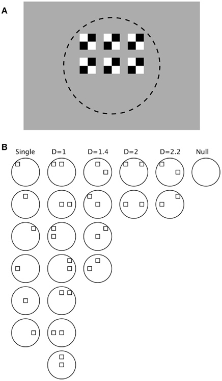
Figure 1. Stimulus configuration. (A) One single stimulus was placed centered in the receptive field (indicated by dashed circle, not shown in the actual display) of each neuron, and five other stimuli were arranged around it separated by a spacing of one-half the stimulus width. Stimuli were black and white and presented on a uniform gray background. (B) Combinations of stimuli included: all six single stimuli, all 15 combinations of two stimuli, and a null stimulus. The paired stimuli were classified according to a normalized distance metric: D = 1 means adjacent stimuli, D = 1.4 means diagonally adjacent stimuli, D = 2 means stimuli two places removed, and D = 2.2 means two spaces horizontal and one vertical.
The receptive field centers ranged from 9.2° to 26.8° from the center of gaze (median 19.1°), and the size of the individual stimuli varied from 0.64° to 1.68° in width. The stimulus combinations were presented in shuffled random order, minimally 20 repetitions, and with a median of 32 repetitions. Trials where the animals did not maintain fixation were not included in these totals and were not analyzed. Rewards were given after every three or four stimulus presentations, and a 3-s interval was inserted after the reward to minimize lick artifact in the spike channel.
While the stimuli were not explicitly optimized for each neuron, only neurons that responded robustly to the single stimuli were used in this study. All neurons had statistically significant responses to single stimuli that were at least twice baseline for at least four of the six locations within the RF, and only five neurons did not meet this criteria for all six locations. The mean spike count for all single stimuli and all neurons was 23.96 spikes/s, and 90% of the mean spike counts were between 4.1 and 50.0 spikes/s.
The stimuli were flashed on for 24 video frames at 85 Hz (approximately 282 ms duration), in a data acquisition window that lasted 440 ms. These 440 ms epochs were separated by intervals that varied randomly from 400 to 800 ms, except when a reward was given. Presenting the stimuli in short temporal epochs is consistent both with the brief duration of inter-saccadic intervals, and with the observed high speed of the visual system (Thorpe et al., 1996). Additionally, for most visual cortical neurons the effects of flashing a stimulus on in the receptive field with the eyes fixed is comparable to having a saccade bring a constant stimulus into the receptive field (Richmond et al., 1999; Gawne and Martin, 2002b). Hence, this paradigm closely approximates the normal operating conditions of primate visual cortical neurons.
The animals were in a controlled behavioral state, performing a fixation task, where all the different stimulus configurations had the same lack of behavioral relevance. It is possible that there could have been uncontrolled covert shifts in attention, but because the stimuli were presented in random order, and because of the short-time analysis intervals, this could not have caused any systematic bias in the results.
Data Analysis
The single-unit responses were quantified by convolving the raw spike times with a Gaussian kernel with a σ = 3 ms, which has the effect of low-pass filtering with a cutoff frequency of 44 Hz. This creates a continuous spike density function (Silverman, 1986), which is essentially a smoothed post-stimulus histogram, but with the advantage that it does not suffer from “bin-edge artifact” (the problem with histograms when changing spike times near the edge of two bins radically alters the appearance of the response). These filter parameters can result in spike density functions with very high peak rates with very few spikes: a burst of just three spikes separated by inter-spike intervals of 3 ms results in peak rates of 300 spikes/s. While lower-frequency cutoff filters increase the precision of estimation of the firing rate over a defined epoch, exploring rapid response dynamics requires high-frequency cutoff filters. This could result in a selection bias for units that produce high-temporal precision firing: using a broader sigma (such as 75 ms as was used in Ghose and Maunsell, 2008), would allow significant responses to be obtained from units that fire at low rates or with low temporal precision relative to stimulus onset times, but would also make it difficult or impossible to study the short-time scale dynamics studied here.
Response latency was defined as the time that it took the response to go halfway from baseline to the maximum of the spike density function in the range of 30–150 ms after stimulus onset. Starting at baseline is a general procedure used for this technique to avoid false triggering for cells with high baselines and low peak responses (Lee et al., 2007). Response magnitude, in mean spikes per second, was also defined during this interval. Using the time to half-maximum response has the advantage that the number of trials per stimulus condition does not influence the measure of latency as compared to using the time where the response surpassed a particular SD (Lee et al., 2007), and has been shown to be a relatively robust and reliable indicator of latency (Levick, 1973). For some cells, latency values could not be assigned for some stimulus cases because few or no spikes were produced, and these data were excluded from any analysis involving latency. The data were resampled with replacement 1000 times, and the latency recalculated each time, which allowed a bootstrapped 95% confidence interval to be calculated.
In order to quantify the interaction between stimuli within the RF of a neuron, we used a response index defined as the spike count for two stimuli presented simultaneously (R12), divided by the maximum of the response to each stimulus of the pair (R1, R2) presented individually.

Thus, a response index value of 1.0 indicates a winner-take-all or “MAX” operation, a value less than 1.0 indicates suppression, and a value greater than 1.0 indicates summation. It has been pointed out that accurately modeling the spatial summation of multiple stimuli within a RF can require models with more free parameters (see Ghose and Maunsell, 2008). However, the purpose of this response index was to provide a simple and robust indicator of the interaction between stimuli. Using more complex models of summation with multiple free parameters per stimulus pair would also have been hard to interpret with more than two locations of stimulus positions within a RF.
All experimental procedures and care of the animals were carried out in compliance with guidelines established by the National Institute of Health and were approved by the University of Alabama at Birmingham Animal Care and Use Committee.
Results
Figure 2 shows example results from three neurons. Each row represents a subset of the results from a single neuron. Each panel illustrates the average spike density function of the responses, overlaying the responses to both stimuli presented separately, and both presented together. The neuron in the topmost row (Figures 2A–D) showed either weighted averaging (Figures 2A,D) or MAX behavior (Figures 2B,C) in the response magnitude. However, for all pairs of stimuli, the response latency was precisely locked to the shortest latency of the responses to both stimuli presented separately. For the neuron in the middle row the response magnitude showed weighted averaging (Figures 2E,H), MAX (Figure 2G), or enhancement (Figure 2F) depending on which pair of stimuli were used. As with the first neuron, the response latency for two stimuli was generally very tightly locked to the shortest latency response of the individual stimuli, but there was one exception (Figure 2E). When the response to a pair of stimuli has a different latency than the shortest latency to one stimulus by itself, this will be termed a latency shift. The third neuron in this example Figures 2I–L also had response magnitude effects that ranged from MAX (Figure 2I), weighted averaging (Figures 2J,L), and enhancement (Figure 2K). However, the latency shifts were more common here: in Figures 2I,J the latency shifts were on the order of 1 ms, and in Figures 2K,L on the order of 8 ms. This neuron showed the highest incidence of latency shifts in the sample population.
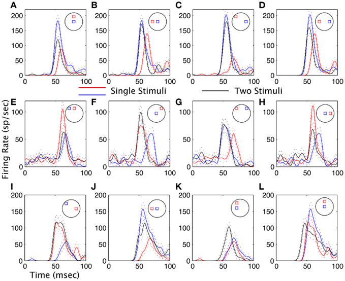
Figure 2. Examples of interactions between stimuli in the receptive fields of visual cortical neurons. (A–D) are from one neuron, and (E–H) from another, and (I–L) from a third. Data are plotted as spike density waveforms as a function of time. Stimulus onset was at time = 0 ms. The configurations of the stimuli are indicated schematically in each panel similar to that shown in Figure 1. Black lines are the responses to both stimuli presented at the same time, and red and blue lines are for each stimulus presented separately. Dashed lines are the mean plus or minus one SE. (A,D) The response to the pair has a magnitude in between the responses to the stimuli presented separately (weighted averaging). (B,C,G) The magnitude of the response to a pair is equal to the magnitude of the larges response to a single stimulus (MAX). (E) In this case the magnitude of the response to both stimuli is closer to the weakest of the two responses, but there is also a strong latency shift. (F) The magnitude of the response to the pair is greater than the response to either stimulus presented separately (summation). (I,J) Latency shifts are on the order of 1 ms. (K,L) Large latency shifts are observed for both summation (K) and suppression (L).
Figure 3 shows summary data from all pair-wise stimulus combinations for all neurons in the study. Figure 3A shows the response index vs. normalized inter-stimulus distance. The tendency across all neurons and all inter-stimulus separation distances was for there to be suppression/averaging, but the range of the results was considerable. Figure 3B shows the same index only this time separated out by individual neuron. Some neurons did tend to have the same sort of interaction for all pairs of stimuli, but most neurons displayed a wide range of different sorts of interactions within their RFs depending on the specific configuration of the stimulus pairs. A one-way ANOVA on the mean response index for each neuron was significant P < 0.001, demonstrating that there was a significant difference between cells in how pairs of stimuli interact in their RFs, but it only explained 27.6% of the variance. In other words, some neurons tend to respond to pairs of stimuli with a degree of consistency, but overall, the results are dominated by the variability within a single neuron.
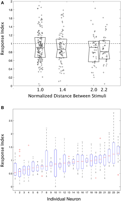
Figure 3. (A) The degree to which two stimuli interact (“Response Index”) in their effect on the responses of a visual cortical neuron, as a function of the normalized distance between stimuli. Each point is from a single pair of stimuli for a single neuron. The Median and ±25% quartile ranges for the data are also shown. (B) The response index plotted as a function of each individual neuron. Some neurons did tend toward one level of response, but overall the trend was weak, and neurons typically showed a wide variety of behavior depending upon the position of the stimuli within their receptive fields.
Figures 4A–C shows plots of response strength vs. response latency for three example neurons. There is an occasional tendency for the weakest responses to have the longest latencies (see Figure 4C), but in general there was no correlation between response strength and latency.
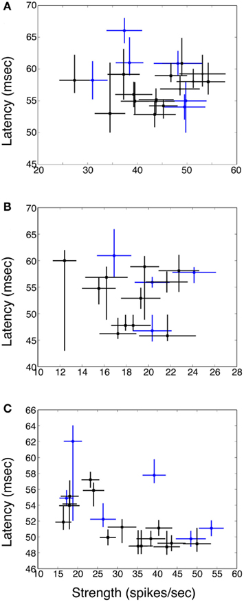
Figure 4. Plot of response latency vs. strength for three example neurons (A–C). Responses to single stimuli are indicated via blue circles; responses to pairs of stimuli via black squares. Horizontal bars are SE of the mean; vertical bars are bootstrapped 95% confidence intervals. In general there is no relationship between response strength and latency. In (C) for the weakest responses latency is prolonged, but this was rarely seen, because for many cells all the responses were relatively robust, and also because for the weakest responses it was often the case that latency could not be defined.
Figure 5A plots the normalized response strength vs. the relative latency shift for all pair-wise stimulus combinations for all neurons in this study. Strength was normalized to the strongest response of any condition for each neuron, and latency is relative to the median latency for each neuron. There is effectively no correlation between the response strength and latency for the stimuli used in this study. Figure 5B illustrates the response latency shift for a pair of stimuli relative to the response shortest latency to either of the two stimuli presented alone. There is a significant dispersion of latency shifts, with a roughly equal tendency for the latencies to be shifted to shorter or longer times. However, there were many cases where the response latency to two stimuli was precisely locked to the shortest of the latencies of to each stimulus presented separately. Note that the distribution is not a Gaussian, but rather has a strong peak at zero phase delay that falls away in an approximately exponential manner, suggesting that there is something special about small latency shifts. The SD of this distribution is large because of outliers (±9.3 ms), but 51.9% of the distribution lies within ±2 ms of zero.
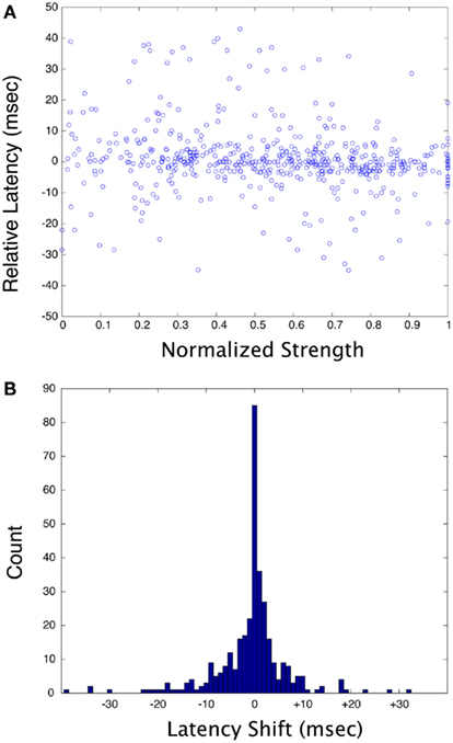
Figure 5. (A) Plots of normalized response strength vs. relative latency for all neurons and all stimulus combinations in this study. For each cell, strength was normalized to the strongest response, and latency was calculated as a difference relative to the median latency. (B) Plot of the shift in latency for the response of a cell to two stimuli, relative to the shortest latency of the response to each stimulus in the pair presented separately. A negative number means that the response to two stimuli has a shorter-latency than the shortest of the response to a single stimulus (this could be considered a phase-advance).
Discussion
At least for the population of neurons and stimulus conditions used in this experiment, there is very little consistency in how the responses to two stimuli are related to the responses to single stimuli. We can consider that the function applied to two visual stimuli is more strongly related to the positions of the stimuli within the RF than it is a fixed property of a specific neuron itself. With hindsight this should not be surprising: two widely separated stimuli may have separate perceptual identities, but when stimuli are in close proximity their relative position should have strong effects on their perceptual meaning and hence on their neural processing. For example, as two separate spots are brought closer together they could start to be treated as a single bar, and different positional shifts could engage end-stopping mechanisms, etc. However, as with most previous studies of this nature, here it was not possible to probe how the monkey perceived the pairs of stimuli, so this remains speculative. Studies where different configurations of stimuli have different behavioral relevance, or are specifically designed to be part of larger forms, may help to answer such questions.
The lack of an effect of the distance of separation between stimuli was unexpected (see Figure 3A), but even those stimuli with the greatest degree of separation were still not as far apart as was the case in previous studies in this lab.
It has been proposed that many cortical neurons perform a single canonical operation on their inputs. For example, the output of a neuron could be driven by the single strongest input, a “winner-take-all” rule (Riesenhuber and Poggio, 1999). However, the results of this study demonstrate that you cannot in general determine the rule by only using two stimulus locations, because the rule could be different for stimuli that are located in different areas of the RF.
It must be emphasized that stimulating a visual cortical neuron with discrete visual stimuli is not the same thing as directly controlling the inputs to that neuron. This is because there are many processing stages between the visual image that is focused on the retina, and a visual cortical neuron, including the processing in the neural retina, thalamus, and any earlier cortical areas. Therefore it is possible that many of the neurons in this study did have a single computational rule that they applied to all of their direct inputs equally, but that the observed sensitivity of the responses to changes in position within the RF was due to interactions between the stimuli at earlier stages in processing.
The lack of correlation between response strength and response latency was striking. As you change the configurations of stimuli inside the RF of a visual cortical neuron, the response strength varies in complicated patterns that presumably reflect aspects of form processing. However, the response latency has a very different pattern of results, and tended to remain fixed as stimuli were combined in different ways. If these neurons were summing up excitatory and inhibitory inputs over some period of time, there should have been a link between strength and latency: for example, if the response to two stimuli was larger than the response to either alone, the response latency should have been shorter. Previous studies have demonstrated a separation of the response magnitude and latency of visual cortical neurons (Carandini and Heeger, 1994; Albrecht, 1995; Gawne et al., 1996; Reich et al., 2001), and the results here are in accord with and extend these previous results. One interpretation is that response strength represents visual form, and that it therefore changes with changes in the relative configuration of the two stimuli in the RF of the neurons. Latency, however, could represent stimulus saliency, and at least under some conditions the saliency of an entire form could be inherited from the most salient single component.
In previous studies from this laboratory, relative response times were varied by either changing the spatial frequency of the stimuli (Gawne and Martin, 2002a; for references to the effects of spatial frequency on response latency see Marr and Poggio, 1979; Nishihara, 1984; Anderson and Van Essen, 1987; Parker et al., 1997; Bredfeldt and Ringach, 2002; Menz and Freeman, 2003; Frazor et al., 2004), or by changing the contrast and also the relative onset timing of the stimuli (Gawne, 2008). Evidence for rapid temporal gating was observed in these studies, where the temporal response to pairs of stimuli was completely dominated by the temporal response to the stimulus that by itself elicited the shortest latency. A similar effect is seen here, in that the response to two stimuli often has the same latency as the shortest single latency response, and there is no second peak in the response to two stimuli that would correspond to the peak of the longer latency response. However, the results of this study showed an important difference from previous studies: the stimulus that by itself elicited the longest response latency could often affect the magnitude of the shorter-latency response, but without always shifting its latency.
It has been proposed that much of cortical computation is performed at the millisecond level using feed-forward circuitry (Delorme and Thorpe, 2001; VanRullen and Thorpe, 2002; VanRullen, 2007; Liu et al., 2009). A consequence of rapid feed-forward processing should be that changing the configuration of the stimuli could change the magnitude of the response, but have little or no effect on the latency of the response (because the computations are so rapid). Therefore, it is hypothesized that for those specific cases when you change the configuration of visual stimuli, and you change the response magnitude of a visual cortical neuron, but you do not change the response latency, this may indicate the involvement of rapid feed-forward processing. On the other hand, imagine a processing mechanism that integrates inputs over a relatively long period of time before generating a response. In this case, changes in response magnitude should often be coupled with significant changes in response latency. It is difficult to conceive of a mechanism that integrates inputs over a long period of time, where changing the inputs results in changes in response magnitude but not latency. Such a system could in principle exist, but it would need to be precisely and deliberately tuned to consistently produce such a result.
Many researchers have argued that much of visual perception is due to a hierarchical feed-forward system of processing (Fukushima, 1980; Rolls, 1991; Riesenhuber and Poggio, 1999; VanRullen and Thorpe, 2002). However, it has also been argued that feedback mechanisms are critical for vision (Lamme and Roelfsema, 2000; Bullier, 2001; Hochstein and Ahissar, 2002; Garrido et al., 2007). More work remains to be done, but it is hypothesized that the relationship between changes in response latency and response magnitude as a stimulus configuration is changed, constitutes a temporal signature that can, at least under some conditions, distinguish between these different mechanisms. At the very least, these results should provide powerful constraints on the development of dynamical models of cortical processing.
Conflict of Interest Statement
The author declares that the research was conducted in the absence of any commercial or financial relationships that could be construed as a potential conflict of interest.
Acknowledgments
This work was supported by the National Science Foundation grant IOS 0622318 (Timothy J. Gawne) and NIH EY03039 (UAB Vision Science Research Center Core). James Black, Jerry Millican, Mark Bolding, Alexander Zotov, and Abidim Yildirim are acknowledged for technical support.
References
Albrecht, D. G. (1995). Visual cortex neurons in monkey and cat; effect of contrast on the spatial and temporal phase transfer functions. Vis. Neurosci. 12, 1191–1210.
Anderson, C. H., and Van Essen, D. C. (1987). Shifter circuits: a computa- tional strategy for dynamic aspects of visual processing. Proc. Natl. Acad. Sci. U.S.A. 84, 6297–6301.
Bredfeldt, C. E., and Ringach, D. L. (2002). Dynamics of spatial frequency tuning in macaque V1. J. Neurosci. 22, 1976–1984.
Carandini, M., and Heeger, D. (1994). Summation and division by neurons in primate visual cortex. Science 264, 1333–1336.
Delorme, A., and Thorpe, S. J. (2001). Face identification using one spike per neuron: resistance to image degradation. Neural Netw. 14, 795–803.
Finn, I. M., and Ferster, D. (2007). Computational diversity in complex cells of cat primary visual cortex. J. Neurosci. 27, 9638–9648.
Frazor, R. A., Albrecht, D. G., Geisler, W. S., and Crane, A. M. (2004). Visual cortex neurons of monkey and cats: temporal dynamics of the spatial frequency response function. J. Neurophysiol. 91, 2607–2627.
Fukushima, K. (1980). Neocognitron: a self organizing neural network model for a mechanism of pattern recognition unaffected by shift in position. Biol. Cybern. 36, 193–202.
Garrido, M. I., Kilner, J. M., Kiebel, S. J., and Friston, K. J. (2007). Evoked brain responses are generated by feedback loops. Proc. Natl. Acad. Sci. U.S.A. 104, 20961–20966.
Gawne, T. J. (2008). Stimulus selection via differential response latencies in visual cortical area V4. Neurosci. Lett. 435, 198–203.
Gawne, T. J. (2010). The local and non-local components of the local field potential in awake primate visual cortex. J. Comput. Neurosci. 29, 615–623.
Gawne, T. J., Kjaer, T. W., and Richmond, B. J. (1996). Latency: another potential code for feature binding in striate cortex. J. Neurophysiol. 76, 1356–1360.
Gawne, T. J., and Martin, J. M. (2002a). Responses of primate visual cortical V4 neurons to simultaneously presented stimuli. J. Neurophysiol. 88, 1128–1135.
Gawne, T. J., and Martin, J. M. (2002b). Responses of primate visual cortical neurons to stimuli presented by flash, saccade, blink, and external darkening. J. Neurophysiol. 88, 2178–2186.
Ghose, G. M., and Maunsell, J. H. R. (2008). Spatial summation can explain the attentional modulation of neuronal responses to multiple stimuli in area V4. J. Neurosci. 28, 5115–5126.
Heuer, H. W., and Britten, K. H. (2002). Contrast dependence of response normalization in area MT of the rhesus macaque. J. Neurophysiol. 88, 3398–3408.
Hochstein, S., and Ahissar, M. (2002). View from the top: hierarchies and reverse hierarchies in the visual system. Neuron 36, 791–804.
Lamme, V. A. F., and Roelfsema, P. R. (2000). The distinct modes of vision offered by feedforward and recurrent processing. Trends Neurosci. 23, 571–579.
Lampl, I., Ferster, D., Poggio, T., and Riesenhuber, M. (2004). Intracellular measurements of spatial integration and the MAX operation in complex cells of the cat primary visual cortex. J. Neurophysiol. 92, 2704–2713.
Lee, J., Williford, T., and Maunsell, J. H. (2007). Spatial attention and the latency and the neuronal responses in macaque area V4. J. Neurosci. 27, 9632–9637.
Levick, W. R. (1973). Variations in the response latency of cat retinal ganglion cells. Vision Res. 13, 837–853.
Liu, H., Agam, Y., Madsen, J. R., and Kreiman, G. (2009). Timing, timing, timing: fast decoding of object information from intracranial field potentials in human visual cortex. Neuron 62, 281–290.
Luck, S. J., Chelazzi, L., Hillyard, S. A., and Desimone, R. (1997). Neural mechanisms of spatial selective attention in areas V1, V2, and V4 of macaque visual cortex. J. Neurophysiol. 77, 24–42.
Marr, D., and Poggio, T. (1979). A computational theory of human stereo vision. Proc. R. Soc. Lond. B Biol. Sci. 204, 301–328.
Menz, M. D., and Freeman, R. D. (2003). Stereoscopic depth processing in the visual cortex: Coarse-to-fine mechanism. Nat. Neurosci. 6, 59–65.
Moran, J., and Desimone, R. (1985). Selective attention gates visual processing in the extrastriate cortex. Science 229, 782–784.
Oleksiak, A., Klink, P. C., Postma, A., van der Ham, I. J. M., Lankheet, M. J., and van Wezel, R. J. A. (2011). Spatial summation in macaque parietal area 7a follows a winner-take-all rule. J. Neurophysiol. 105, 1150–1158.
Parker, D. M., Lishman, J. R., and Hughes, J. (1997). Evidence for the view that temporospatial integration in vision is temporally anisotropic. Perception 26, 1169–1180.
Reich, D. S., Mechler, F., and Victor, J. D. (2001). Temporal coding of contrast in primary visual cortex: when, what, and why? J. Neurophysiol. 85, 1039–1050.
Reynolds, J. H., Chelazzi, L., and Desimone, R. (1999). Competitive mechanisms subserve attention in macaque areas V2 and V4. J. Neurosci. 19, 1736–1753.
Reynolds, J. H., and Desimone, R. (2003). Interacting roles of attention and visual salience in V4. Neuron 37, 853–863.
Richmond, B. J., Hertz, J. A., and Gawne, T. J. (1999). The relation between V1 neuronal responses and eye movement-like stimulus presentations. Neurocomputing 26–27, 247–254.
Riesenhuber, M., and Poggio, T. (1999). Hierarchical models of object recognition in cortex. Nat. Neurosci. 2, 1019–1025.
Rolls, E. T. (1991). Neural organization of higher visual functions. Curr. Opin. Neurobiol. 1, 274–278.
Rolls, E. T., Aggelopoulos, N. C., and Zheng, F. (2003). The receptive fields of inferior temporal cortex neurons in natural scenes. J. Neurosci. 23, 339–348.
Sato, T. (1989). Interactions of visual stimuli in the receptive fields of inferior temporal neurons in awake macaques. Exp. Brain Res. 77, 23–30.
Silverman, B. W. (1986). Density Estimation for Statistics and Data Analysis. New York, NY: Chapman and Hall.
Thorpe, S. J., Fize, D., and Marlot, C. (1996). Speed of processing in the human visual system. Nature 381, 520–522.
VanRullen, R., and Thorpe, S. J. (2002). Surfing a spike wave down the ventral stream. Vis. Res. 42, 2593–2615.
Keywords: V2, latency, max, winner-take-all, feedback
Citation: Gawne TJ (2011) Short-time scale dynamics in the responses to multiple stimuli in visual cortex. Front. Psychology 2:323. doi: 10.3389/fpsyg.2011.00323
Received: 03 May 2011; Accepted: 21 October 2011;
Published online: 08 November 2011.
Edited by:
Gabriel Kreiman, Harvard, USAReviewed by:
Bartlett W. Mel, University of Southern California, USAThomas Miconi, Centre National de la Recherche Scientifique, France
Jorge Almeida, University of Minho, Portugal
Copyright: © 2011 Gawne. This is an open-access article subject to a non-exclusive license between the authors and Frontiers Media SA, which permits use, distribution and reproduction in other forums, provided the original authors and source are credited and other Frontiers conditions are complied with.
*Correspondence: Timothy J. Gawne, Department of Vision Sciences, University of Alabama at Birmingham, 924 South 18th Street, Birmingham, AL 35294, USA. e-mail:dGdhd25lQGdtYWlsLmNvbQ==