 Le Yu
Le Yu Yifei Dai3†
 Yan Ji
 Huan Si
 Lirui Cheng
 Tao Zhao
 Yanjun Zan
- 1Tobacco Research Institute, Chinese Academy of Agricultural Sciences, Qingdao, China
- 2Department of Plant Biology, Swedish University of Agriculture Sciences, Uppsala, Sweden
- 3Department of Population and Public Health Sciences, Keck School of Medicine, University of Southern California, Los Angeles, CA, United States
- 4College of Ecology, Lanzhou University, Lanzhou, China
- 5College of Horticulture, Northwest Agriculture and Forestry University, Yangling, China
Genomic prediction is a powerful approach for improving genetic gain and shortening the breeding cycles in animal and crop breeding programs. A series of statistical and machine learning models has been developed to increase the prediction performance continuously. However, the application of these models requires advanced R programming skills and command-line tools to perform quality control, format input files, and install packages and dependencies, posing challenges for breeders. Here, we present ShinyGS, a stand-alone R Shiny application with a user-friendly interface that allows breeders to perform genomic selection through simple point-and-click actions. This toolkit incorporates 16 methods, including linear models from maximum likelihood and Bayesian framework (BA, BB, BC, BL, and BRR), machine learning models, and a data visualization function. In addition, we benchmarked the performance of all 16 models using multiple populations and traits with varying populations and genetic architecture. Recommendations were given for specific breeding applications. Overall, ShinyGS is a platform-independent software that can be run on all operating systems with a Docker container for quick installation. It is freely available to non-commercial users at Docker Hub (https://hub.docker.com/r/yfd2/ags).
1 Introduction
Polygenic traits are influenced by multiple genes, leading to continuously distributed phenotypes, such as plant height, grain yield, and resistance to diseases. Accurate predictions of these traits can help crop and animal breeders develop varieties and breeds with significantly improved agronomic performance to meet the growing food demand (Bali and Singla, 2022). Over the past two decades, genomic selection (GS) has become a popular strategy for animal and plant breeding programs and considerably improved the genetic gain for many crops and animals (Liu et al., 2018; Lozada et al., 2019; Marulanda et al., 2016; Sallam and Smith, 2016; Schefers and Weigel, 2012). Various methods have been developed to improve prediction accuracy and computing efficacy (Habier et al., 2011; Jia and Jannink, 2012; Meuwissen et al., 2001; VanRaden, 2008). However, the application of these models requires advanced R programming skills and command-line tools for performing data quality control, formatting input files, and installing dependencies and packages, posing challenges for many breeders.
To make these advanced genomic prediction methods accessible to breeders without programming skills, we developed ShinyGS—a graphical toolkit with a series of genetic and machine learning models for genomic selection. It includes 16 genomic prediction methods implemented in four packages: ridge regression best linear unbiased prediction (rrBLUP) (Meuwissen et al., 2001), the most widely used method based on linear regression models; deep neural network genomic prediction (DNNGP) (Wang et al., 2023); gradient boosting machine (GBM) (Li et al., 2018); and the BWGS (Breed Wheat Genomic Selection pipeline including several genomic prediction methods) (Charmet et al., 2020) method set. DNNGP is based on a deep multilayered hidden neural network architecture that captures complex non-additive effects (Wang et al., 2023). The GBM method utilizes gradient boosting (Friedman, 2001) and stochastic gradient boosting approaches (Friedman, 2002). The BWGS package includes the genomic best linear unbiased prediction (G-BLUP) (VanRaden, 2008), multiple kernel reproducing kernel Hilbert space (MKRKHS) (De Los Campos et al., 2010), ridge regression (RR) (Whittaker et al., 2000), Bayesian ridge regression (BRR) (De Los Campos et al., 2013), least absolute shrinkage and selection operator (LASSO) (Usai et al., 2009), elastic net (EN) (Zou and Hastie, 2005), Bayesian LASSO (BL) (Park and Casella, 2008), Bayes A (BA) (Meuwissen et al., 2001), Bayes B (BB) (Habier et al., 2011), Bayes C (BC) (George and McCulloch, 1993), reproducing kernel Hilbert space (RKHS) (Gianola and van Kaam, 2008), random forest (RF) (Breiman, 2001), and support vector machine (SVM) (González-Recio et al., 2014; Maenhout et al., 2007) models (Table 1). In addition, we performed benchmarking analysis using multiple populations and traits with variable population and genetic architecture to provide recommendations for specific breeding applications. ShinyGS is freely available to non-commercial users at Docker Hub (https://hub.docker.com/r/yfd2/ags). This toolkit can significantly simplify genomic prediction applications, making advanced genomic selection methods more accessible and beneficial to breeders.

Table 1. Description of each model.
2 Materials and methods
2.1 Example data
Genetic relationship is one of the most important factors that may affect prediction accuracy of genomic selection. As population structure varies between advanced intercross line or germplasm, we choose two types of population to demonstrate the performance of these models. The first is the Goodman maize diversity panel. This panel was built from whole-genome sequencing data from approximately 300 maize lines, covering major maize varieties across the world (Bukowski et al., 2018). Genotypes were downloaded from https://datacommons.cyverse.org/browse/iplant/home/shared/commons_repo/curated/Qi_Sun_Zea_mays_haplotype_map_2018/hmp321_unimputed. We downloaded phenotype records for days to anthesis (DTA), plant height (PH), and ear weight (EW) from Panzea (traitMatrix_maize282NAM_v15-130212.txt) with 282 observations.
For the maize CUBIC population, all 1,404 lines were resequenced. Genotype data were available for download from Liu et al. (2020) (The raw fastq files were uploaded to NCBI SRA with ID as PRJNA597703 and called SNP data in PLINK format available at https://pan.baidu.com/s/1AsPJLTe–gU5EN8aFTMYPA). We downloaded phenotype records for DTA, PH, and EW from Liu et al. (2020) with 1,404 observations.
2.2 Genotype filtering
A comprehensive genotype filtration was performed to ensure data quality and reliability. Initially, genotype data were extracted from the VCF file and converted into PLINK binary format. A minor allele frequency (MAF) filter was applied, retaining SNPs with an MAF greater than 0.05 to exclude rare variants. Next, linkage disequilibrium (LD) pruning was conducted to remove SNPs in high LD, using an r2 threshold of 0.9 within a sliding window of 1,000 base pairs. The resulting dataset was recoded to a raw genotype file. Prediction accuracy was calculated as the correlation of phenotype and predicted breeding value.
2.3 Model implementation
ShinyGS integrates multiple GS algorithms from various packages: rrBLUP, BWGS, GBM, and DNNGP. The rrBLUP, BWGS, and GBM packages are implemented in R libraries, whereas DNNGP is called from a Python module. The rrBLUP method is from the “rrBLUP” package. It is a fast maximum-likelihood algorithm for mixed models, assuming that all markers have equal variance with small but non-zero effects (Endelman, 2011). This model estimates the marker effects from training datasets and ultimately estimates the genomic estimated breeding values (GEBVs) for the selection of candidates. BWGS is an integrated package compiling various R libraries for easy computation of (GEBV) (Charmet et al., 2020). The GBLUP, MKRKHS, RR, BRR, LASSO, EN, BL, BA, BB, BC, RF, and SVM models are included in this package. The GBM method is from the “gbm” package (Ridgeway, 2007). It mainly takes the gradient boosting (Friedman, 2001) and stochastic gradient boosting approaches (Friedman, 2002). This method is especially appropriate for mining less than clean data. DNNGP is a Python pipeline, developed based on deep neural network-based method. It can be used to predict phenotypes of plants based on multi-omics data (Wang et al., 2023).
3 Results and discussion
3.1 ShinyGS application overview
ShinyGS is an R shiny application integrating a series of genetic and machine learning models for genomic selection. The application interface comprises four main sections: Model Selection, Data Upload, Parameter Adjustment, and Data Visualization. This application includes 16 genomic prediction algorithms, including rrBLUP, DNNGP, GBM, GBLUP, MKRKHS, RR, LASSO, EN, BRR, BL, BA, BB, BC, RKHS, RF, and SVM, for users to select in the “Model Selection” panel (Figure 1). Users can upload genotype data files in VCF format and phenotype data files in TXT format via the “Data Upload” panel. Upon uploading the correct files, a “Run Analysis” button appears. Users can adjust model parameters based on the selected genomic prediction models. After the analysis is completed, a scatterplot with predicted breeding values and raw phenotype is generated, and a table with predicted breeding values can be downloaded in the “Data Visualization” panel (Figure 1).
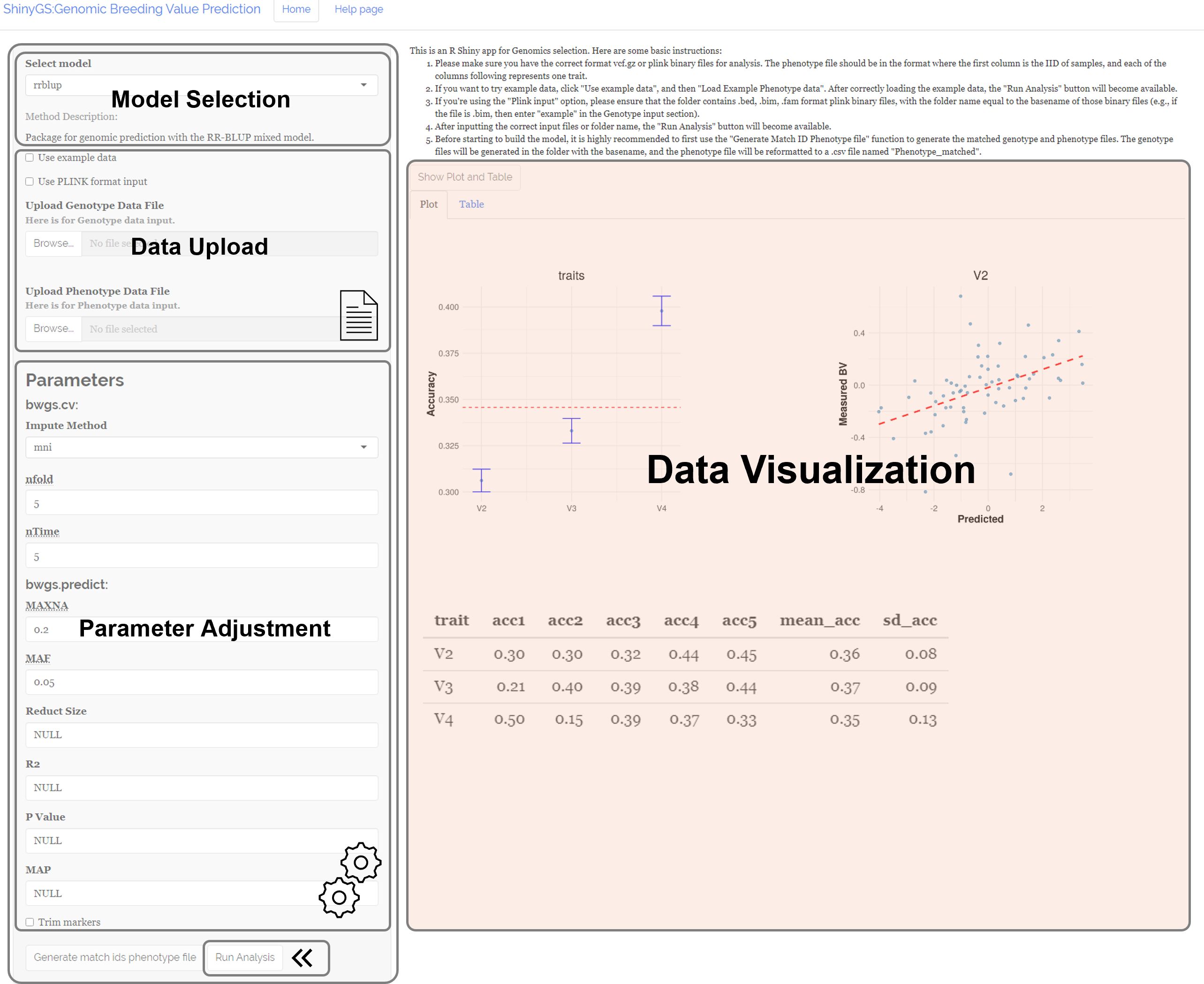
Figure 1. Work panel of the ShinyGS application.
3.2 Demonstration of ShinyGS functionalities
In this section, we will demonstrate the functionalities using a maize diversity panel with 282 resequenced genotypes and measured days to flowering (DTF).
i. Model Selection: A total of 16 models are available for selection from the drop-down tab in the “Select Model” panel (Figure 2).
ii. Parameter Adjustment: For models without any additional parameters, such as the rrBLUP model, the “Parameter Adjustment” panel does not appear when these models are selected. Otherwise, a parameter adjustment panel will show up. For example, when using the BWGS method set, users can set the imputation method, max NA, MAF, size reduction, R2, P-value, and MAP. When using the DNNGP model, users can set batch size, learning rate, number of epochs, first dropout, second dropout, patience for learning rate reduction, random seed, number of folders for cross-validation, part for validation set, early stopping threshold, and number of PCA.
iii. Data Upload: Users can upload genotype and phenotype files in the Data Upload section. Both “.vcf” and “.vcf.gz” file formats are acceptable for genotype files. A vcf file contains genetic markers for genomic selection. For phenotype files, ShinyGS accepts both “.txt” and “.csv” formats, with IDs in the first column. Raw phenotype needs to be preprocessed accordingly before it can be pushed into our software. The phenotype file could include a header with ID and trait names. However, this is not mandatory. Input phenotypes without a header will be assigned with a header starting with a V-column number. ShinyGS links input genotype and phenotype files with IDs, so it is important to make sure that IDs in the two files are consistent. If not, users can create an ID-matched phenotype file using the “Generate match IDs phenotype file” function. Alternatively, ShinyGS also accepts genotype and phenotype in PLINK format. This can be done by checking the “Use PLINK format input” box and input the folder name with PLINK files into the genotype box.
iv. Run Analysis: Once the above steps are completed, a “Run Analysis” button appears.
v. Results and Visualization: After the analysis is completed, a scatterplot with predicted breeding values and raw phenotype is generated, and a table with predicted breeding values can be downloaded.
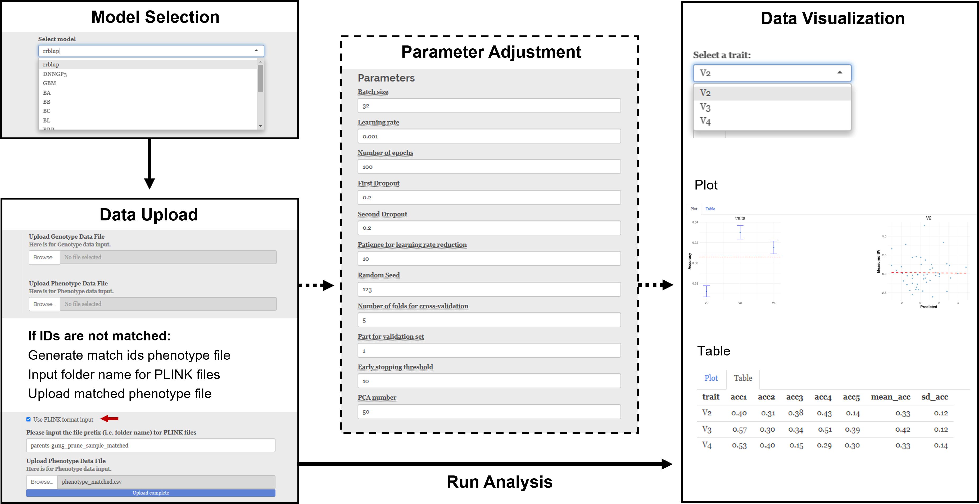
Figure 2. Demonstration of ShinyGS by predicting DTF in a maize diversity panel with 282 recombination intercross populations (RILs).
3.3 Benchmarking model performances for a number of traits using a recombination intercross population
In this section, we benchmarked the performance of the 16 models using a maize multiple parental advanced intercross population (CUBIC) (Liu et al., 2020). This population was derived from 24 elite Chinese maize inbred lines from four divergent heterotic groups, and a total of 24 founders were crossed under a complete diallel cross-mating design (Liu et al., 2020). After selfing for more than 10 generations, a total of 1,404 inbred maize lines were obtained, genotyped, and phenotyped. Here, 42,267 single nucleotide polymorphisms (SNPs) and three traits—PH (cm), DTA (days), and EW (g)—were used. Prediction accuracy was calculated as the Pearson correlation between measured phenotype and predicted breeding values.
For PH, the prediction accuracy varied from 0.52 to 0.60, with an average of 0.57 (Figure 3). The MKRKHS model displays the highest accuracy (0.60), while the LASSO model displays the lowest accuracy (0.52). For DTA, the average prediction accuracy is 0.52, and the SVM, DNNGP, and GBM models show accuracies lower than 0.5 (Figure 3). Due to relatively low heritability, the average accuracy for the EW dataset is 0.31 with MKRKHS yielding the highest prediction performance (Figure 3).
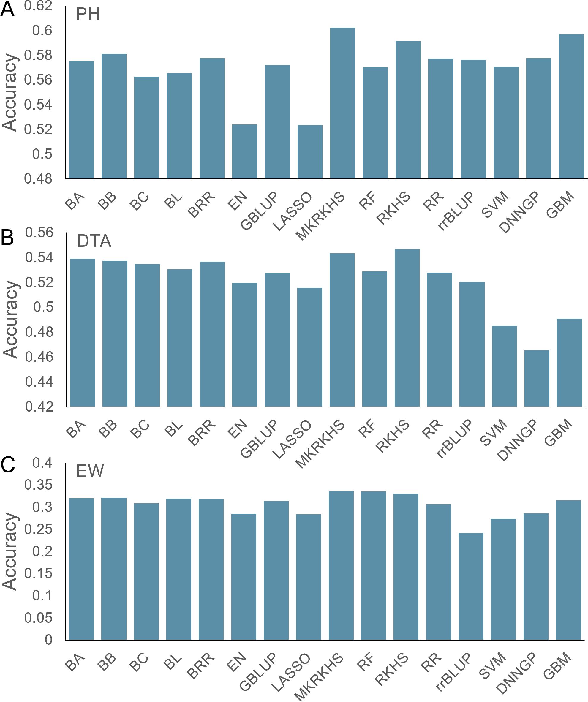
Figure 3. Prediction accuracy of 16 models for the maize CUBIC population. (A) PH, (B) DTA, and (C) EW.
Although the prediction accuracies varied between traits and models, MKRKHS showed the highest accuracies for all three traits. We, therefore, recommend using the MKRKHS model as a first choice in intercross population in future applications.
3.4 Benchmarking model performances for a number of traits using a maize diversity panel
In this section, we benchmarked the performance of the 16 models using the maize Goodman diversity panel, which included 26 stiff stalk lines, 103 non-stiff stalk lines, 77 tropical/subtropical lines, 6 sweet corn lines, 9 popcorn lines, and 61 mixed lines (Kremling et al., 2018). Compared with the CUBIC population, this population is highly stratified, covering major Zea mays varieties across the world. There were 16,238 SNPs, and three phenotypes—DTA (days), PH (cm), and EW (g)—were used.
The average accuracies for the three phenotypes across the 16 models were 0.84, 0.55, and 0.64, respectively (Figures 4A–C). Compared with the other models, EN and LASSO had lower accuracy in all three tests. Although the prediction accuracies varied between traits and models, the GBM model showed the highest accuracies for all three traits. We, therefore, recommend using the GBM model as the first choice in a diversified population in future applications.
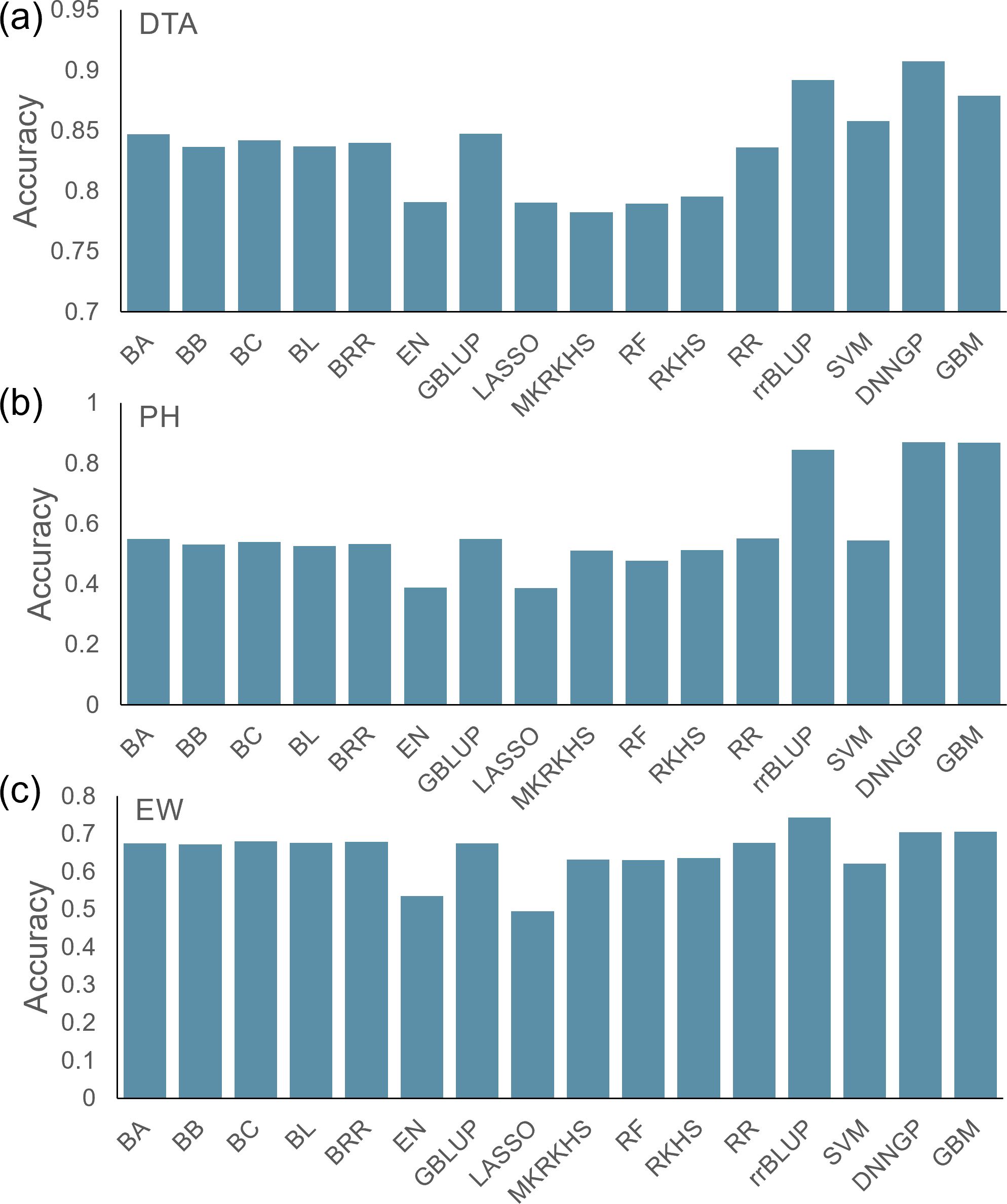
Figure 4. Prediction accuracy of 16 models for the maize Goodman diversity panel. (A) DTA, (B) PH, and (C) EW.
3.5 Comparison of computing time and memory usage
In this section, we benchmarked computing time and memory usage in relation to population size and prediction methods. To estimate how computational resource scales with population size for each method, we calculated computing time and memory consumption by downsampling the CUBIC population to 500, 800, and 1,404 individuals.
Overall, most models displayed increased computing time with a larger population size. There are two models, RF and MKRKHS, that took more than 500 min, regardless of population size. The RF model took a longer computing time than the other models, and its time consumption increases linearly as the population grows (Figure 5).
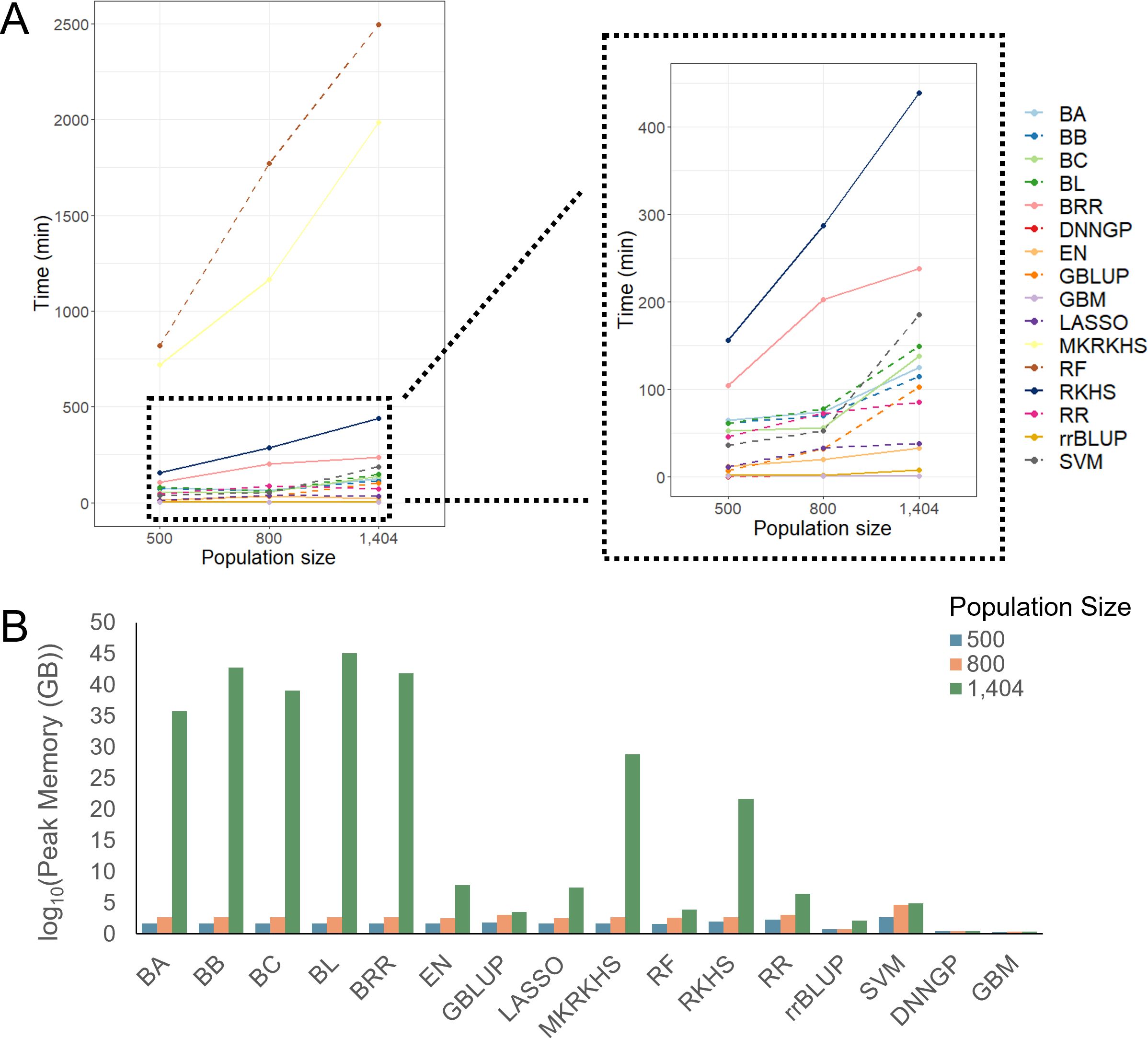
Figure 5. Computing time and memory usage of different models with different population sizes. (A) Computing time of 16 models. (B) Memory usage of 16 models.
For memory usage, most models used less than 3 GB memory at population sizes of 500 and 800 but increased sharply at a population size of 1,404. The GBLUP and SVM models used the largest amount of memory at a population size of 800. In contrast, the DNNGP and GBM models showed stable memory usage (Figure 5).
Overall, Bayesian methods scale poorly with sample size and cannot outperform other methods in nearly all the benchmarked traits and populations. We suggest users to leave them as the last option. Taking the prediction performance, computational time, and resources together, GBM could be the first choice as it gives satisfying performance under reasonable time especially when computational resources are limited. Under limited computational resources and time, RF and MKRKHS should be the last option as they are associated with much higher costs in time and resources with no or marginal gain in accuracy. Overall, we suggest users balance the prediction accuracy and available computational resources in their breeding applications.
Data availability statement
The original contributions presented in the study are included in the article/Supplementary Material. Further inquiries can be directed to the corresponding authors.
Author contributions
LY: Data curation, Formal analysis, Visualization, Writing – original draft, Writing – review & editing. YD: Data curation, Formal analysis, Methodology, Software, Writing – review & editing. MZ: Data curation, Formal analysis, Methodology, Software, Writing – review & editing. LG: Formal analysis, Writing – review & editing. YJ: Formal analysis, Writing – review & editing. HS: Formal analysis, Writing – review & editing. LC: Writing – review & editing. TZ: Conceptualization, Writing – review & editing. YZ: Conceptualization, Funding acquisition, Writing – original draft, Writing – review & editing.
Funding
The author(s) declare that financial support was received for the research, authorship, and/or publication of this article. This research was funded by the State Key Research and Development Project-Youth Scientist program (2023YFD1202400), National Science Foundation of China (32200503), Taishan Young Scholar Program and Distinguished Overseas Young Talents Program from Shandong Province (2024HWYQ-079), and Agricultural Science and Technology Innovation Program (ASTIP-TRIC01) from the Chinese Academy of Agricultural Sciences. The authors declare that this study received funding from Key Science and Technology Project from China National Tobacco Corporation (110202101040 JY-17). The funder was not involved in the study design, collection, analysis, interpretation of data, the writing of this article or the decision to submit it for publication.
Conflict of interest
The authors declare that the research was conducted in the absence of any commercial or financial relationships that could be construed as a potential conflict of interest.
Publisher’s note
All claims expressed in this article are solely those of the authors and do not necessarily represent those of their affiliated organizations, or those of the publisher, the editors and the reviewers. Any product that may be evaluated in this article, or claim that may be made by its manufacturer, is not guaranteed or endorsed by the publisher.
Supplementary material
The Supplementary Material for this article can be found online at: https://www.frontiersin.org/articles/10.3389/fpls.2024.1480902/full#supplementary-material
References
Bali, N., Singla, A. (2022). Emerging trends in machine learning to predict crop yield and study its influential factors: A survey. Arch. Comput. Methods Eng. 29, 95–112. doi: 10.1007/s11831-021-09569-8
Bukowski, R., Guo, X., Lu, Y., Zou, C., He, B., Rong, Z., et al. (2018). ). Construction of the third-generation Zea mays haplotype map. GigaScience 7, gix134. doi: 10.1093/gigascience/gix134
Charmet, G., Tran, L.-G., Auzanneau, J., Rincent, R., Bouchet, S. (2020). BWGS: A R package for genomic selection and its application to a wheat breeding programme. PloS One 15, e0222733. doi: 10.1371/journal.pone.0222733
De Los Campos, G., Gianola, D., Rosa, G. J. M., Weigel, K. A., Crossa, J. (2010). Semi-parametric genomic-enabled prediction of genetic values using reproducing kernel Hilbert spaces methods. Genet. Res. 92, 295–308. doi: 10.1017/S0016672310000285
De Los Campos, G., Hickey, J. M., Pong-Wong, R., Daetwyler, H. D., Calus, M. P. L. (2013). Whole-genome regression and prediction methods applied to plant and animal breeding. Genetics 193, 327–345. doi: 10.1534/genetics.112.143313
Endelman, J. B. (2011). Ridge regression and other kernels for genomic selection with R package rrBLUP. Plant Genome 4, 250–255. doi: 10.3835/plantgenome2011.08.0024
Friedman, J. H. (2001). Greedy function approximation: A gradient boosting machine. Ann. Stat 29, 1189–1232. doi: 10.1214/aos/1013203451
Friedman, J. H. (2002). Stochastic gradient boosting. Comput. Stat Data Anal. 38, 367–378. doi: 10.1016/S0167-9473(01)00065-2
George, E. I., McCulloch, R. E. (1993). Variable selection via gibbs sampling. J. Am. Stat. Assoc. 88, 881–889. doi: 10.2307/2290777
Gianola, D., van Kaam, J. B. C. H. M. (2008). Reproducing kernel hilbert spaces regression methods for genomic assisted prediction of quantitative traits. Genetics 178, 2289–2303. doi: 10.1534/genetics.107.084285
González-Recio, O., Rosa, G. J. M., Gianola, D. (2014). Machine learning methods and predictive ability metrics for genome-wide prediction of complex traits. Livestock Sci. 166, 217–231. doi: 10.1016/j.livsci.2014.05.036
Habier, D., Fernando, R. L., Kizilkaya, K., Garrick, D. J. (2011). Extension of the bayesian alphabet for genomic selection. BMC Bioinf. 12, 186. doi: 10.1186/1471-2105-12-186
Jia, Y., Jannink, J.-L. (2012). Multiple-trait genomic selection methods increase genetic value prediction accuracy. Genetics 192, 1513–1522. doi: 10.1534/genetics.112.144246
Kremling, K. A. G., Chen, S.-Y., Su, M.-H., Lepak, N. K., Romay, M. C., Swarts, K. L., et al. (20187697). Dysregulation of expression correlates with rare-allele burden and fitness loss in maize. Nature 555, 520–523. doi: 10.1038/nature25966
Li, F., Zhang, L., Chen, B., Gao, D., Cheng, Y., Zhang, X., et al. (2018). A Light Gradient Boosting Machine for remainning useful life estimation of aircraft engines. 2018 21st International Conference on Intelligent Transportation System (Itsc). 3562–3567.
Liu, H. J., Wang, X. Q., Xiao, Y. J., Luo, J. Y., Qiao, F., Yang, W. Y., et al. (2020). A CUBIC: an atlas of genetic architecture promises directed maize improvement. Genome Biol. 21. doi: 10.1186/s13059-020-1930-x
Liu, X., Wang, H., Wang, H., Guo, Z., Xu, X., Liu, J., et al. (2018). Factors affecting genomic selection revealed by empirical evidence in maize. Crop J. 6, 341–352. doi: 10.1016/j.cj.2018.03.005
Lozada, D. N., Mason, R. E., Sarinelli, J. M., Brown-Guedira, G. (2019). Accuracy of genomic selection for grain yield and agronomic traits in soft red winter wheat. BMC Genet. 20, 82. doi: 10.1186/s12863-019-0785-1
Maenhout, S., De Baets, B., Haesaert, G., Van Bockstaele, E. (2007). Support vector machine regression for the prediction of maize hybrid performance. Theor. Appl. Genet. 115, 1003–1013. doi: 10.1007/s00122-007-0627-9
Marulanda, J. J., Mi, X., Melchinger, A. E., Xu, J.-L., Würschum, T., Longin, C. F. H. (2016). Optimum breeding strategies using genomic selection for hybrid breeding in wheat, maize, rye, barley, rice and triticale. Theor. Appl. Genet. 129, 1901–1913. doi: 10.1007/s00122-016-2748-5
Meuwissen, T. H. E., Hayes, B. J., Goddard, M. E. (2001). Prediction of total genetic value using genome-wide dense marker maps. Genetics 157, 1819–1829. doi: 10.1093/genetics/157.4.1819
Park, T., Casella, G. (2008). The bayesian lasso. J. Am. Stat. Assoc. 103, 681–686. doi: 10.1198/016214508000000337
Ridgeway, G. J. U. (2007). 'Generalized boosted models: A guide to the gbm package'. R package version 2.1.1.
Sallam, A. H., Smith, K. P. (2016). Genomic selection performs similarly to phenotypic selection in barley. Crop Sci. 56, 2871–2881. doi: 10.2135/cropsci2015.09.0557
Schefers, J. M., Weigel, K. A. (2012). Genomic selection in dairy cattle: Integration of DNA testing into breeding programs. Anim. Front. 2, 4–9. doi: 10.2527/af.2011-0032
Usai, M. G., Goddard, M. E., Hayes, B. J. (2009). LASSO with cross-validation for genomic selection. Genet. Res. 91, 427–436. doi: 10.1017/S0016672309990334
VanRaden, P. M. (2008). Efficient methods to compute genomic predictions. J. Dairy Sci. 91, 4414–4423. doi: 10.3168/jds.2007-0980
Wang, K., Abid, M. A., Rasheed, A., Crossa, J., Hearne, S., Li, H. (2023). DNNGP, a deep neural network-based method for genomic prediction using multi-omics data in plants. Mol. Plant 16, 279–293. doi: 10.1016/j.molp.2022.11.004
Whittaker, J. C., Thompson, R., Denham, M. C. (2000). Marker-assisted selection using ridge regression. Genetical Res. 75, 249–252. doi: 10.1017/S0016672399004462
Keywords: genomic prediction, BLUP, machine learning, breeding, graphical toolkit
Citation: Yu L, Dai Y, Zhu M, Guo L, Ji Y, Si H, Cheng L, Zhao T and Zan Y (2024) ShinyGS—a graphical toolkit with a serial of genetic and machine learning models for genomic selection: application, benchmarking, and recommendations. Front. Plant Sci. 15:1480902. doi: 10.3389/fpls.2024.1480902
Received: 14 August 2024; Accepted: 02 December 2024;
Published: 24 December 2024.
Edited by:
George V. Popescu, Mississippi State University, United StatesReviewed by:
Juliana Petrini, Clinica do Leite Ltda, BrazilGuoqing Tang, Sichuan Agricultural University, China
Copyright © 2024 Yu, Dai, Zhu, Guo, Ji, Si, Cheng, Zhao and Zan. This is an open-access article distributed under the terms of the Creative Commons Attribution License (CC BY). The use, distribution or reproduction in other forums is permitted, provided the original author(s) and the copyright owner(s) are credited and that the original publication in this journal is cited, in accordance with accepted academic practice. No use, distribution or reproduction is permitted which does not comply with these terms.
*Correspondence: Tao Zhao, dGFvLnpoYW9AbndhZnUuZWR1LmNu; Yanjun Zan, emFueWFuanVuQGNhYXMuY24=
†These authors have contributed equally to this work