Research on noise prediction methods for sound barriers based on the integration of conditional generative adversarial networks and numerical methods

This study proposes a novel approach utilizing Conditional Generative Adversarial Networks (CGANs) to accelerate wideband acoustic state analysis, addressing the computational challenges in traditional Boundary Element Method (BEM) approaches. Traditional BEM-based acoustic analysis requires repeated computation of frequency-dependent system matrices across multiple frequencies, leading to significant computational costs. The asymmetry and full-rank nature of the BEM coefficient matrices further increase computational demands, particularly in large-scale problems. To overcome these challenges, this paper introduces a CGAN-based modeling framework that significantly reduces computation time while maintaining high predictive accuracy. The framework demonstrates exceptional adaptability when handling datasets with varying characteristics, effectively capturing underlying patterns within the data. Numerical experiments validate the effectiveness of the proposed method, highlighting its advantages in both accuracy and computational efficiency. This CGAN-based approach provides a promising alternative for efficient wideband acoustic analysis, significantly reducing computation time while ensuring accuracy.

1 Introduction

In the field of acoustics, the simulation and analysis of sound wave propagation through complex structures [1, 2] are of paramount importance. Frequency sweep calculations [3] are crucial for understanding the behavior of sound waves across a range of frequencies, which is essential for designing effective acoustic barriers and noise reduction devices. Traditional computational methods typically employ the Finite Element Method (FEM) [4–6] or the Boundary Element Method (BEM) [7–10]. Among these, BEM [11]is widely recognized for its superior accuracy and simplicity in mesh generation [12–14], making it a preferred method for addressing acoustic problems. Its natural compliance with the Sommerfeld radiation condition at infinity further solidifies its utility in external acoustic analyses [15], [9].

Conventional sound pressure calculations are typically optimized for specific frequencies, limiting their application across broader frequency ranges. To address this limitation, broadband analysis [16] has been introduced, enabling the computation of results over a wider frequency spectrum. However, in broadband analysis [17–19], the frequency band is divided into segments, necessitating the recalculation of the coefficient matrix and boundary element system [20, 21], equations for each frequency. This process imposes a significant computational burden. Recent advancements in computational power and data-driven methods have spurred the development of neural networks [22–25], presenting promising opportunities for accelerating complex acoustic analyses. For example, [26] proposed a noise prediction model for wing structures, while [27] utilized Deep Neural Networks (DNN) to expedite uncertainty quantification in vibro-acoustic coupling analysis. These studies underscore the potential of neural networks in acoustic modeling and analysis.

This paper introduces an efficient method for accelerating frequency sweep calculations in broadband acoustics using Conditional Generative Adversarial Networks (CGANs) [28]. By employing CGANs, the computational overhead inherent in broadband analysis is significantly reduced. Generative Adversarial Networks (GANs) [29–32], initially proposed as a framework for training generative models, offer several advantages: eliminating the need for Markov chains, relying solely on backpropagation for gradient computation, avoiding inference during learning, and easily integrating various factors and interactions. However, a major limitation of GANs is their inability to control the modes of generated data in an unconditional model.

In contrast, Conditional Generative Adversarial Networks (CGANs) incorporate a conditioning variable, enabling control over the generative process and constraining outputs to a user-defined distribution. This enhancement improves model stability. The adversarial training mechanism in CGANs not only ensures accurate and realistic data generation but also uncovers the underlying relationships within the data [33–36]. These capabilities make CGANs particularly suitable for acoustic scattering problems characterized by complex distribution features. This study focuses on integrating CGANs with traditional numerical methods to predict the acoustic scattering characteristics of barriers, thereby reducing computational complexity, accelerating computations, and establishing new surrogate models for acoustic scattering analysis [37, 38].

Neural network-based prediction methods are widely adopted across various fields due to their dynamic capabilities [39–42]. These methods leverage learning algorithms that achieve high prediction accuracy by iterative training on simulated sound pressure and sensitivity data. A key advantage of this approach is its ability to construct highly nonlinear models [43–45], making it particularly effective for complex noise analysis. Additionally, these methods reduce computational workloads, provide high-precision predictions, and meet the demands of rapid analysis in engineering applications. As technology continues to advance, neural network-based methods have evolved rapidly, finding applications across numerous disciplines.

Significant research progress in machine learning-driven sound pressure [46] prediction has been made in recent years, both domestically and internationally. Applications such as robotic fish, noise barrier models, and submarines demonstrate the engineering relevance of these advancements. In 2023, [47] applied deep neural networks and Catmull-Clark subdivision surfaces [48, 49] to perform vibro-acoustic analysis on various geometric models, achieving sound pressure responses across multiple parameters and dimensions. That same year, [50] used Loop subdivision surfaces to model the robotic fish “Manta” and predicted the effects of geometric and material parameters on sound pressure.

To improve the efficiency of broadband optimization and apply CGANs to 2D acoustic problems, this paper presents the following contributions:

$•$ Development of a CGAN-based network for predicting data, such as sound pressure.

$•$ Validation of the CGAN network’s performance through an infinitely long rigid model and an acoustic barrier model.

The structure of this paper is as follows: Section 2 outlines the boundary element integral equations, while Section 3 details the theory of CGAN networks and their loss functions. Section 4.1 validates the accuracy and efficiency of CGAN predictions using the infinitely long rigid cylinder model, and Section 4.2 demonstrates the feasibility of CGAN networks as surrogate models for acoustic scattering analysis through an acoustic barrier model.

2 Acoustic boundary element method

Consider the Helmholtz equation for a 2D acoustic problem, given as Equation 1.

${\nabla }^{2}p\left(\mathbf{x}\right)+k^{2}p\left(\mathbf{x}\right)=0,\forall \mathbf{x}\in \mathrm{\Omega }(1)$

The Helmholtz half-space problem can be represented by the following BIE and normal derivative boundary integral equation (HBIE).

$C\left(\mathbf{x}\right)p\left(\mathbf{x}\right)+{\int }_{S}F\left(\mathbf{x},\mathbf{y}\right)p\left(\mathbf{y}\right)\mathrm{d}S\left(\mathbf{y}\right)={\int }_{S}G\left(\mathbf{x},\mathbf{y}\right)q\left(\mathbf{y}\right)\mathrm{d}S\left(\mathbf{y}\right)+p_{\text{inc}}\left(\mathbf{x}\right)(2)$

and

$C\left(\mathbf{x}\right)q\left(\mathbf{x}\right)+{\int }_{S}H\left(\mathbf{x},\mathbf{y}\right)p\left(\mathbf{y}\right)\mathrm{d}S\left(\mathbf{y}\right)={\int }_{S}K\left(\mathbf{x},\mathbf{y}\right)q\left(\mathbf{y}\right)\mathrm{d}S\left(\mathbf{y}\right)+\frac{\partial p_{\text{inc}}\left(\mathbf{x}\right)}{\partial n\left(\mathbf{x}\right)}(3)$

where $\mathbf{y}$ signifies the field point, $\mathbf{x}$ denotes the source point, and $q$ is the normal derivative of the sound pressure $p$: $q(\mathbf{x})=\partial p(\mathbf{x})/\partial n(\mathbf{x})$. When $\mathbf{x}$ is located on a border that is smooth $S$, $C(\mathbf{x})=1/2$. Acoustic pressure incident at position $\mathbf{x}$ is given by $p_{\mathit{inc}}(\mathbf{x})$. Green’s function $G(\mathbf{x},\mathbf{y})$ and its derivative in Equation 2 and Equation 3 are presented as follows

$\left\{\begin{array}{c}G\left(\mathbf{x},\mathbf{y}\right)=\frac{\text{i}}{4}{H}_0^{\left(1\right)}\left(kr\right)\hfill \\ \hfill \\ F\left(\mathbf{x},\mathbf{y}\right)=\frac{\partial G\left(\mathbf{x},\mathbf{y}\right)}{\partial n\left(\mathbf{y}\right)}=-\frac{\text{i}k}{4}{H}_1^{\left(1\right)}\left(kr\right)\frac{\partial r}{\partial n\left(\mathbf{y}\right)}\hfill \\ \hfill \\ K\left(\mathbf{x},\mathbf{y}\right)=\frac{\partial G\left(\mathbf{x},\mathbf{y}\right)}{\partial n\left(\mathbf{x}\right)}=-\frac{\text{i}k}{4}{H}_1^{\left(1\right)}\left(kr\right)\frac{\partial r}{\partial n\left(\mathbf{x}\right)}\hfill \\ \hfill \\ H\left(\mathbf{x},\mathbf{y}\right)=\frac{{\partial }^{2}G\left(\mathbf{x},\mathbf{y}\right)}{\partial n\left(\mathbf{x}\right)\partial n\left(\mathbf{y}\right)}=\frac{\text{i}k}{4r}{H}_1^{\left(1\right)}\left(kr\right)n_j\left(\mathbf{x}\right)n_j\left(\mathbf{y}\right)-\frac{\text{i}{k}^2}{4}{H}_2^{\left(1\right)}\left(kr\right)\frac{\partial r}{\partial n\left(\mathbf{x}\right)}\frac{\partial r}{\partial n\left(\mathbf{y}\right)}\hfill \end{array}\right.(4)$

where the $n$th order first kind Hankel function is indicated by $H_n^{(1)}$, $k$ denotes by the wave number, $\text{i}=\sqrt{-1}$, $n_j$ is the Cartesian component of $n(\mathbf{x})$ or $n(\mathbf{y})$ and the distance between the field and source locations is represented by the formula $r=\left|\mathbf{x}-\mathbf{y}\right|$.

For exterior acoustic problems, using either Equation 2 or Equation 3 alone can lead to non-uniqueness of the solution at certain imaginary frequencies. According to the Burton-Miller idea, a linear combination of Equation2 and Equation 3 can effectively resolve this issue. The Burton-Miller formulation is expressed as follows

$\begin{array}{ll}\hfill & C\left(\mathbf{x}\right)\left[p\left(\mathbf{x}\right)+\alpha q\left(\mathbf{x}\right)\right]+{\int }_S\left[F\left(\mathbf{x},\mathbf{y}\right)+\alpha H\left(\mathbf{x},\mathbf{y}\right)\right]p\left(\mathbf{y}\right)\mathrm{d}S\left(\mathbf{y}\right)\hfill \\ \hfill & ={\int }_S\left[G\left(\mathbf{x},\mathbf{y}\right)+\alpha K\left(\mathbf{x},\mathbf{y}\right)\right]q\left(\mathbf{y}\right)\mathrm{d}S\left(\mathbf{y}\right)+p_{\mathrm{i}\mathrm{n}\mathrm{c}}\left(\mathbf{x}\right)+\alpha \frac{\partial p_{\mathrm{i}\mathrm{n}\mathrm{c}}\left(\mathbf{x}\right)}{\partial n\left(\mathbf{x}\right)}\hfill \end{array}(5)$

in which $\alpha$ represents the coupling parameter: defined as $\alpha =\text{i}/k$ where $k>1$ and $\alpha =\text{i}$ in other cases.

By discretizing the structural boundary into several elements using constant elements and introducing the coefficient matrix, Equation 5 can be reformulated as follows

$\mathbf{H}\mathbf{p}-\mathbf{G}\mathbf{q}={\mathbf{p}}_f^{\text{inc}}(6)$

where $\mathbf{H}$ and $\mathbf{G}\in {\mathbb{C}}^{N\times N}$ ($N$ indicates the number of degrees of freedom.) are the coefficient matrices. They are asymmetric, fully populated, and frequency-related. The column vectors $\mathbf{p}$ and $\mathbf{q}$, respectively, represent the sound pressure and the acoustic flux at the collocation locations. ${\mathbf{p}}_f^{\text{inc}}$ is the vector of the incident wave. To determine the sound pressure values at the boundary surface nodes, Equation 6 needs to be solved. Subsequently, the sound pressure can be computed at any point within the acoustic domain by using Equation 5 with $\alpha =0$ and $C(\mathbf{x})=1$.

Its sound pressure, ${\mathbf{p}}_f$, can be written as follows if the computation takes into account the external acoustic field.

${\mathbf{p}}_f=-\left|{\mathbf{H}}_f\mathbf{p}-{\mathbf{G}}_f\mathbf{q}\right|+{\mathbf{p}}_f^{\mathit{inc}}(7)$

where the matrices ${\mathbf{H}}_f$ and ${\mathbf{G}}_f$ as well as the vector ${\mathbf{p}}_f^{\mathit{inc}}$ are similar to those in Equation 6, except that the source point $\mathbf{x}$ is outside the structure domain.

2.1 BEM formulas for shape sensitivity analysis of acoustics

To derive the general formula for acoustic sensitivity analysis by the direct differentiation method, we first differentiate Equation 5 to obtain.

$\begin{array}{ll}\hfill C\left(\mathbf{x}\right)\left[\dot{p}\left(\mathbf{x}\right)+\alpha \dot{q}\left(\mathbf{x}\right)\right]& +{\int }_S\left[\dot{F}\left(\mathbf{x},\mathbf{y}\right)+\alpha \dot{H}\left(\mathbf{x},\mathbf{y}\right)\right]p\left(\mathbf{y}\right)\mathrm{d}S\left(\mathbf{y}\right)\hfill \\ \hfill & +{\int }_S\left[F\left(\mathbf{x},\mathbf{y}\right)+\alpha H\left(\mathbf{x},\mathbf{y}\right)\right]\dot{p}\left(\mathbf{y}\right)\mathrm{d}S\left(\mathbf{y}\right)\hfill \\ \hfill & +{\int }_S\left[F\left(\mathbf{x},\mathbf{y}\right)+\alpha H\left(\mathbf{x},\mathbf{y}\right)\right]p\left(\mathbf{y}\right)\mathrm{d}\dot{S}\left(\mathbf{y}\right)\hfill \\ \hfill & ={\int }_S\left[\dot{G}\left(\mathbf{x},\mathbf{y}\right)+\alpha \dot{K}\left(\mathbf{x},\mathbf{y}\right)\right]q\left(\mathbf{y}\right)\mathrm{d}S\left(\mathbf{y}\right)\hfill \\ \hfill & +{\int }_S\left[G\left(\mathbf{x},\mathbf{y}\right)+\alpha K\left(\mathbf{x},\mathbf{y}\right)\right]\dot{q}\left(\mathbf{y}\right)\mathrm{d}S\left(\mathbf{y}\right)\hfill \\ \hfill & +{\int }_S\left[G\left(\mathbf{x},\mathbf{y}\right)+\alpha K\left(\mathbf{x},\mathbf{y}\right)\right]q\left(\mathbf{y}\right)\mathrm{d}\dot{S}\left(\mathbf{y}\right)\hfill \\ \hfill & +{\dot{p}}_{\mathrm{i}\mathrm{n}\mathrm{c}}\left(\mathbf{x}\right)+\alpha \frac{\partial {\dot{p}}_{\mathrm{i}\mathrm{n}\mathrm{c}}\left(\mathbf{x}\right)}{\partial n\left(\mathbf{x}\right)}\hfill \end{array}(8)$

The basic solution and its derivatives are determined by the coordinates of the field and source points. Therefore, under continuous shape modification, their values might be impacted by a change in a form design variable. In general, the sensitivities of the coordinates can be used to express $\dot{G}$, $\dot{F}$, $\dot{K}$, $\dot{H}$, $\dot{p}$ and $\dot{q}$.

$\left\{\begin{array}{c}\dot{G}\left(\mathbf{x},\mathbf{y}\right)=-\frac{\text{i}k}{4}{H}_1^{\left(1\right)}\left(kr\right)\dot{r}\hfill \\ \hfill \\ \dot{F}\left(\mathbf{x},\mathbf{y}\right)=-\frac{\text{i}k}{4}{H}_1^{\left(1\right)}\left(kr\right)\left[\frac{\left({\dot{\mathbf{y}}}_j-{\dot{\mathbf{x}}}_j\right)n_j\left(\mathbf{y}\right)}{r}+r_{,j}{\dot{n}}_j\left(\mathbf{y}\right)\right]\hfill \\ +\frac{\text{i}{k}^2}{4}{H}_2^{\left(1\right)}\left(kr\right)\dot{r}{r}_{,j}{n}_j\left(\mathbf{y}\right)\hfill \\ \hfill \\ \dot{K}\left(\mathbf{x},\mathbf{y}\right)=-\frac{\text{i}k}{4}{H}_1^{\left(1\right)}\left(kr\right)\left[\frac{\left({\dot{\mathbf{y}}}_j-{\dot{\mathbf{x}}}_j\right)n_j\left(\mathbf{x}\right)}{r}+r_{,j}{\dot{n}}_j\left(\mathbf{x}\right)\right]\hfill \\ +\frac{\text{i}{k}^2}{4}{H}_2^{\left(1\right)}\left(kr\right)\dot{r}{r}_{,j}{n}_j\left(\mathbf{x}\right)\hfill \\ \hfill \\ \dot{H}\left(\mathbf{x},\mathbf{y}\right)=\frac{\text{i}k}{4r}{H}_1^{\left(1\right)}\left(kr\right)\left[{\dot{n}}_j\left(\mathbf{x}\right)n_j\left(\mathbf{y}\right)+n_j\left(\mathbf{x}\right){\dot{n}}_j\left(\mathbf{y}\right)\right]\hfill \\ +\frac{\text{i}{k}^3}{4}{H}_3^{\left(1\right)}\left(kr\right)\dot{r}{r}_{,j}{n}_j\left(\mathbf{x}\right)r_{,l}{n}_l\left(\mathbf{y}\right)\hfill \\ -\frac{\text{i}{k}^2}{4}{H}_2^{\left(1\right)}\left(kr\right)\frac{n_j\left(\mathbf{x}\right)n_j\left(\mathbf{y}\right)\dot{r}}{r}\hfill \\ -\frac{\text{i}{k}^2}{4}{H}_2^{\left(1\right)}\left(kr\right)r_{,j}{n}_j\left(\mathbf{x}\right)\left[{\dot{r}}_{,l}{n}_l\left(\mathbf{y}\right)+r_{,l}{\dot{n}}_l\left(\mathbf{y}\right)\right]\hfill \\ -\frac{\text{i}{k}^2}{4}{H}_2^{\left(1\right)}\left(kr\right)r_{,l}{n}_l\left(\mathbf{y}\right)\left[{\dot{r}}_{,l}{n}_j\left(\mathbf{x}\right)+r_{,l}{\dot{n}}_j\left(\mathbf{x}\right)\right]\hfill \\ -\frac{\text{i}{k}^2}{4}{H}_2^{\left(1\right)}\left(kr\right)\frac{2\dot{r}{r}_{,j}{n}_j\left(\mathbf{x}\right)r_{,l}{n}_l\left(\mathbf{y}\right)}{r}\hfill \end{array}\right.(9)$

where Equations 10, 11 express the details of Equations 9.

$\dot{r}=r_{,j}\left({\dot{\mathbf{y}}}_j-{\dot{\mathbf{x}}}_j\right)(10)$

${\dot{r}}_{,l}{n}_l\left(\mathbf{y}\right)+r_{,l}{\dot{n}}_l\left(\mathbf{y}\right)=\frac{\left({\dot{\mathbf{y}}}_l-{\dot{\mathbf{x}}}_l\right)n_l\left(\mathbf{y}\right)}{r}-\frac{\dot{r}{r}_{,l}{n}_l\left(\mathbf{y}\right)}{r}+r_{,j}{\dot{n}}_l\left(\mathbf{y}\right)(11)$

where $\dot{()}$ indicates differentiation concerning the design variables. Once the form design variable has fully parameterized the border of the studied domain, ${\dot{\mathbf{x}}}_j$ and ${\dot{\mathbf{y}}}_j$ will be assessed. ${\dot{n}}_l(\mathbf{y})$ and $\mathrm{d}\dot{S}(\mathbf{y})$ can be written as Equations 12, 13

${\dot{n}}_l\left(\mathbf{y}\right)=-{\dot{\mathbf{y}}}_{j,l}{n}_j\left(\mathbf{y}\right)+{\dot{\mathbf{y}}}_{j,m}{n}_j\left(\mathbf{y}\right)n_m\left(\mathbf{y}\right)n_l\left(\mathbf{y}\right)(12)$

and

$\mathrm{d}\dot{S}\left(\mathbf{y}\right)=\left[{\dot{\mathbf{y}}}_{l,l}-{\dot{\mathbf{y}}}_{l,j}{n}_l\left(\mathbf{y}\right)n_j\left(\mathbf{y}\right)\right]\mathrm{d}S\left(\mathbf{y}\right)(13)$

where the partial derivatives concerning the coordinate component are indicated by an index following a comma, such as ${\dot{\mathbf{y}}}_{j,m}=\partial {\dot{\mathbf{y}}}_j/\partial {\mathbf{y}}_m$.

The following matrix-form linear algebraic equations are obtained by discretizing Equation 8 using the constant boundary element and gathering the equations for each collocation point.

$\mathbf{H}\dot{\mathbf{p}}+\dot{\mathbf{H}}\mathbf{p}-\mathbf{G}\dot{\mathbf{q}}-\dot{\mathbf{G}}\mathbf{q}={\dot{\mathbf{p}}}_{\text{inc}}(14)$

where $\dot{\mathbf{H}}$ and $\dot{\mathbf{G}}\in {\mathbb{C}}^{N\times N}$ (The number of degrees of freedom is indicated by $N$.) are the coefficient matrices. They are fully populated, asymmetric, and dependent on frequency. The column vectors $\dot{\mathbf{p}}$ and $\dot{\mathbf{q}}$ represent the sensitivity of the acoustic flux and the sound pressure, respectively. ${\dot{\mathbf{p}}}_{\text{inc}}$ represents the sensitivity vector of incident waves.

To determine all the unknown boundary state values for the analysis of shape sensitivity, solve Equation 6 and use all the values at the boundaries and known boundary sensitivity values to solve Equation 14. By Equation 8, the value for any point $\mathbf{x}$ in the problem domain can be computed with $\alpha =0$ and $C(\mathbf{x})=1$. In the end, the sensitivities of the objective function presented at certain computing points in the fluid domain concerning shape design variables could be calculated.

Since the Hankel function in Equation 4 and its derivative in Equation 9 depend on the wave number $k$, Equation 6, Equation 7 and Equation 14 are all dependent on frequency. The computation of the system equation and coefficient matrix of the BEM for 2D acoustic state and sensitivity analysis at each discrete frequency point within a frequency band is necessary, which results in a significant computational cost for tackling multifrequency problems.

3 Theory of conditional generative adversarial networks

3.1 Generate adversarial neural networks

The innovation of Generative Adversarial Networks (GANs) lies in their combination of deep learning and probability theory. They are made up of two rival neural networks that are capable of autonomous learning and are intended to use unsupervised learning to replicate the distribution of actual data [51, 52]. The generator and discriminator engage in an iterative training process that resembles a game, where the generator aims to produce data that closely resembles real data, while the discriminator continuously improves its ability to distinguish between real and generated data. Together, they form the fundamental architecture of GANs. The goal is to make the generated data as similar as possible to the characteristics of the actual data [53]. The generator aims to create data that closely resembles real data to deceive the discriminator, while the discriminator’s role is to distinguish between real data and the fake data produced by the generator. As they strive toward achieving a Nash equilibrium in game theory-where the produced data is indistinguishable from actual data-both networks are always learning and improving. Figure 1 displays the GAN’s process flowchart.

Figure 1

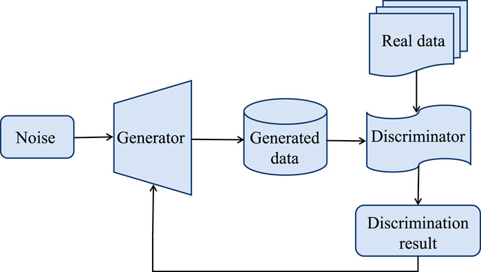
Figure 1. GAN network structure diagram.

The generator takes random noise as input and generates samples resembling the distribution of real data [54]. The discriminator receives either real data or fake data produced by the generator. When the input is real data, the discriminator outputs 1; when the input is generated data, it outputs 0. Both the discriminator’s and the generator’s capabilities are continually enhanced by iterative training, leading to a balanced state where the discriminator is unable to discriminate between the two input data categories. This indicates that the generator has successfully simulated the distribution of real data. The loss value of a GAN is closely tied to the loss values of both the generator and the discriminator, and its loss function can be expressed as Equation 15.

$\underset{G}{\min }\underset{D}{\max }V\left(D,G\right)={\mathit{E}}_{x\sim P_{\text{data}}\left(x\right)}\left[\log D\left(x\right)\right]+{\mathit{E}}_{z\sim P_z\left(z\right)}\left[\log \left(1-D\left(G\left(z\right)\right)\right)\right](15)$

In this context, $P_{\mathit{\text{data}}}(\cdot )$ and $P_z(\cdot )$ represent the distributions of the sample data and noise data, respectively. However, GANs still have a number of difficulties, though, such as non-synchronous training between the discriminator and generator, poor data accuracy, high sample variability, and trouble reaching a level of stability. The CGAN architecture is used in this study to overcome these constraints. A thorough overview of CGAN will be given in the sections that follow.

3.2 Conditional generation adversarial neural network

By adding conditional information, the Conditional Generative Adversarial Network (CGAN) [55] improves on the classic GAN architecture and successfully converts it from an unsupervised learning model to a model with supervised learning. CGAN constrains the data production process by adding conditional variables, which allows for the targeted and accurate generation of desired outputs. The CGAN’s design is quite similar to that of a typical GAN, as seen in Figure 2, but it incorporates extra conditional variables in the discriminator and generator. Because of this improvement, CGAN can function as a supervised, regulated network model.

Figure 2

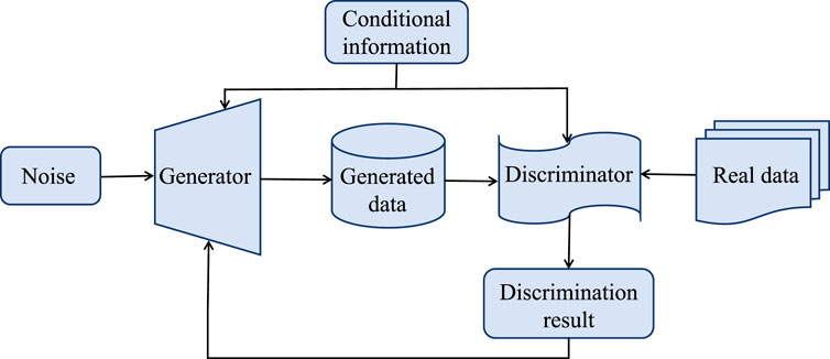
Figure 2. CGAN network structure diagram.

In Equation 16, the CGAN’s goal function is shown, where conditional probability is introduced to form a constrained maximization-minimization function.

$\underset{G}{\min }\underset{D}{\max }V\left(D,G\right)={\mathit{E}}_{x\sim P_{\text{data}}\left(x\right)}\left[\log D\left(x|y\right)\right]+{\mathit{E}}_{z\sim P_z\left(z\right)}\left[\log \left(1-D\left(G\left(z|y\right)\right)\right)\right](16)$

After incorporating conditional variables, the discriminator and generator in CGAN are tasked with two key responsibilities: the discriminator must distinguish between real and generated data under specified conditions, while the generator aims to produce data that aligns with the real data distribution under those same conditions. Random noise and the associated conditional information are inputs to the generative model, generating samples that mimic the distribution of real data. Conversely, the discriminator receives real data, conditional information, and the generated sample $G(y,z)$ as input, outputting either 0 or 1 to classify the input as real or generated. Fundamentally, the discriminator functions as a binary classification model. This structured approach effectively addresses the limitations of GANs.

During the adversarial optimization process, the generator and discriminator continuously refine their performance, ultimately achieving a state of equilibrium where the discriminator can no longer differentiate between real and generated data. The training process for CGAN alternates between updating the generator and the discriminator, linking the overall loss function to the individual loss functions of both components. This relationship is represented in Equation 17:

$L\left(G,D\right)={\mathit{E}}_{x,y,P_{\mathit{data}}\left(x,y\right)}\left[\log D\left(x,y\right)\right]+{\mathit{E}}_{y,p_y\left(y\right),z,p_z\left(z\right)}\left[\log \left(1-D\left(G\left(y,z\right),y\right)\right)\right](17)$

In this context, $x$ represents the real data, $y$ denotes the conditional information, and $P_{\mathit{data}}(x,y)$ indicates the distribution of the input data. The functions $D(\cdot )$ and $G(\cdot )$ represent the outputs of the discriminator $D$ and the generator $G$, respectively, while $z$ denotes the random noise. The loss functions for $D$ and $G$ can be expressed as Equation 18 and Equation 19:

$L_D=-{\mathit{E}}_{x,y,P_{\mathit{data}}\left(x,y\right)}\left[\log D\left(x,y\right)\right]-{\mathit{E}}_{z,p_z,y,p_y\left(z,y\right)}\left[\log \left(1-D\left(G\left(z,y\right)\right),y\right)\right](18)$

$L_G={\mathit{E}}_{z,p_z,y,p_y\left(z,y\right)}\left[\log \left(1-D\left(G\left(z,y\right)\right),y\right)\right](19)$

It is important to note that, due to its generative nature, CGAN has the ability to produce a wide range of data. This generated data also contributes to the training process of the network, which significantly reduces the amount of data required for modeling. As a result, the CGAN network is well-suited to address the issues examined in this paper. Compared to other neural networks, CGAN can be applied to small-scale data problems. However, the training time is slightly longer than that of other neural network models.

4 Numerical example

This section presents two computational examples to evaluate the performance of the proposed algorithm. The acoustic scattering data were generated using numerical simulations implemented in the Fortran 90 programming language. The dataset was subsequently divided into training and testing sets for the CGAN. Figure 3 illustrates the training process of the entire CGAN network, which can be systematically divided into two primary stages. All computations were conducted on a laptop equipped with 16 GB of RAM and an Intel(R) Core(TM) i5-9300H Central Processing Unit (CPU).

Figure 3

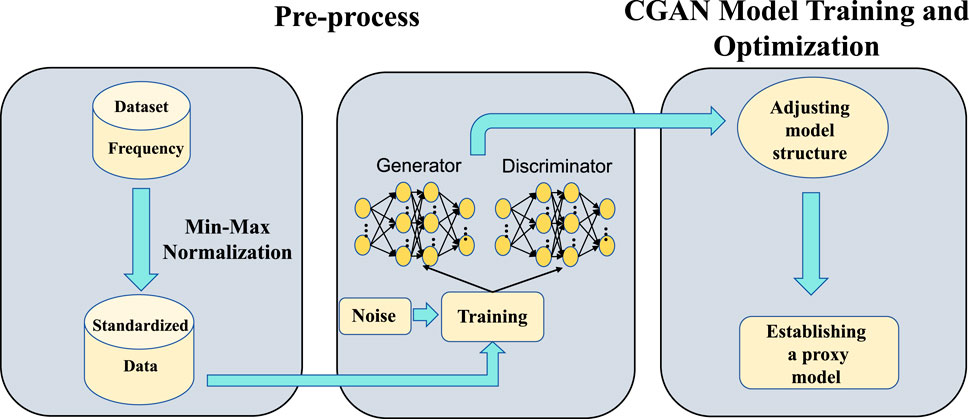
Figure 3. CGAN network structure diagram.

4.1 Infinite-length rigid cylinder model

The acoustic scattering from a cylinder can be simplified to a two-dimensional problem by assuming that a plane wave beam strikes an infinitely rigid cylinder (see Figure 4). The plane wave propagates along the positive $x$-axis. The cylinder is centered at (0 m, 0 m) with a radius of 1 m, and its circumference is discretized using 720 constant boundary elements. Additionally, the coordinates of the calculation points are (10 m, 0 m) (see Figure 4). Other parameters for the numerical simulation are provided in Table 1. The problem of acoustic scattering by an infinitely rigid cylinder has the analytical solution, which is represented as Equation 20.

$p\left(r,\theta \right)=-{\displaystyle \sum _{n=0}^{\infty }}{\epsilon }_n{\mathrm{i}}^n\frac{n{J}_n\left(k{r}_0\right)-k{r}_0{J}_{n+1}\left(k{r}_0\right)}{n{H}_n^{\left(1\right)}\left(k{r}_0\right)-k{r}_0{H}_{n+1}^{\left(1\right)}\left(k{r}_0\right)}{H}_n^{\left(1\right)}\left(kr\right)\cos \left(n\theta \right)(20)$

Figure 4

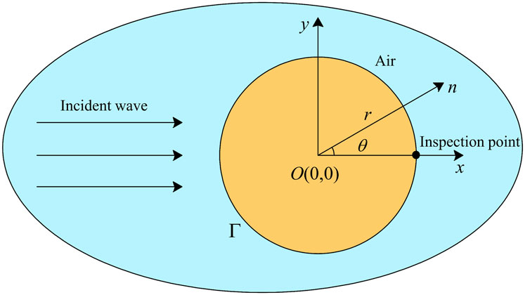
Figure 4. The infinite cylinder serves as the design domain for sound scattering.

Table 1

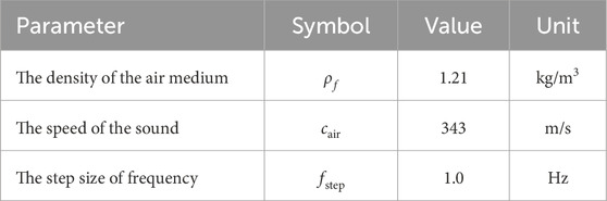
Table 1. Parameters used in the simulations.

In the above equation, ${\epsilon }_0=1$ for $n=0$, and ${\epsilon }_n=2$ otherwise, where ${\epsilon }_n$ represents the Neumann symbols. The expansion consists of 50 terms, and at the detection point, $\theta =0$. To assess the accuracy of the proposed method, the relative error between the traditional Boundary Element Method (DBEM) and the analytical solution, and that between the CGAN-predicted results and the analytical solution, have been calculated. The relative error is determined using Equation 21:

$\mathrm{R}\mathrm{e}\mathrm{l}\mathrm{a}\mathrm{t}\mathrm{i}\mathrm{v}\mathrm{e}\mathrm{E}\mathrm{r}\mathrm{r}\mathrm{o}\mathrm{r}=\frac{\left|X_{\mathit{output}}-X_{\mathit{analytical}}\right|}{\left|X_{\mathit{analytical}}\right|}\times 100\%(21)$

Here, $X_{\text{output}}$ represents the results obtained from DBEM-CGAN, and $X_{\text{analytical}}$ represents the results of the analytical solution. Before training the neural network, data preprocessing is essential. First, a portion of the dataset is randomly selected as the test set to evaluate the model post-training. Additionally, to enhance training efficiency and prediction accuracy by addressing the scale differences among features, data standardization is a critical step. Standardization not only improves the model’s adaptability across different datasets but also increases its sensitivity to feature variations, thereby improving its generalization capability. The standardization process can be implemented using Equation 22:

$x^{\prime }=\frac{x-x_{\min }}{x_{\max }-x_{\min }}(22)$

In this context, $x^{\prime }$ represents the value of a single data point, $x_{\min }$ is the minimum value in the corresponding column, and $x_{\max }$ is the maximum value in that column. After standardization, all features in the dataset are rescaled to a uniform range, ensuring that differences in feature magnitudes do not affect model training and prediction. The standardized dataset is then divided into two subsets: the training set, used to train the model, and the test set, employed to evaluate its performance. Following evaluation, the predicted outputs are post-processed as described in Equation 23.

$x=x^{\prime }\cdot \left(x_{\max }-x_{\min }\right)+x_{\min }(23)$

Based on the acquired dataset (sound pressure and sensitivity from 100Hz to 500 Hz), the data is input into the CGAN model for training. Figures 5, 6 present a simplified diagram of the CGAN structure, illustrating the discriminator’s and generator’s training procedure. $Z_1$ and $Z_2$ represent the random noise inputs to the generator, and $y$ denotes the label information corresponding to the frequency information of the real data. The generated data $x_1$ symbolizes the sensitivity and sound pressure at the observing point. In the discriminator, $x_2$ represents the real data, $\widehat{y}$ represents the label information of the generated data corresponding to its frequency information, and $\widehat{d}$ represents the discrimination result, stating if the data is fake or true.

Figure 5

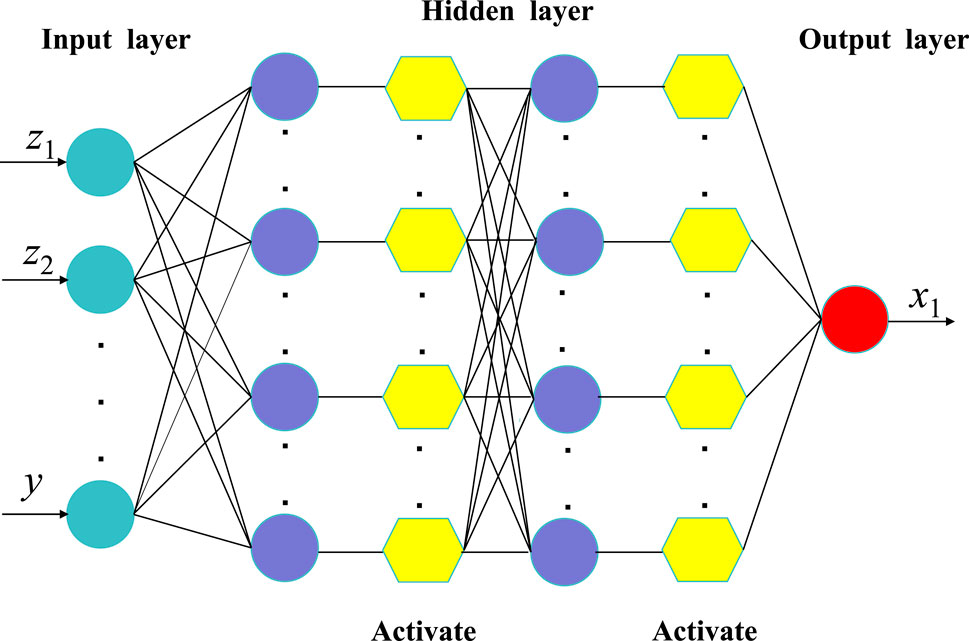
Figure 5. The Generator’s network structure of CGAN.

Figure 6

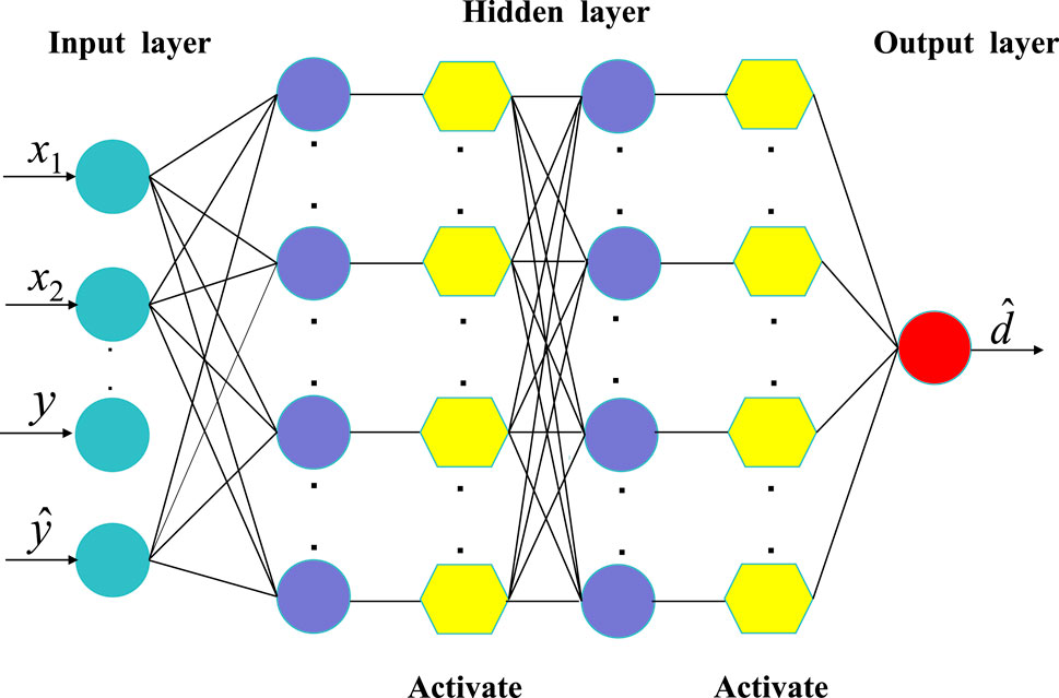
Figure 6. The Discriminator’s network structure of CGAN.

For the tasks of sound pressure and sensitivity prediction, these can be considered a regression problem. Thus, the mean squared error (MSE) function is employed as the loss function, as shown in Equation 24. Since the discriminator operates as a binary classifier, the Sigmoid function is used as the activation function. To ensure balanced performance between the generator and discriminator, the same activation function is applied to both. Additionally, the parameter dimensions are kept within a compact range to enhance the model’s efficiency.

Figure 7 illustrates the variation in the generator’s training loss under different learning rates and optimizers, while Figure 8 demonstrates the impact of the number of hidden layers on the training loss.

$\mathrm{M}\mathrm{S}\mathrm{E}=\frac{1}{n}{\displaystyle \sum _{i=1}^n}{\left({\widehat{y}}_i-y_i\right)}^2(24)$

Figure 7

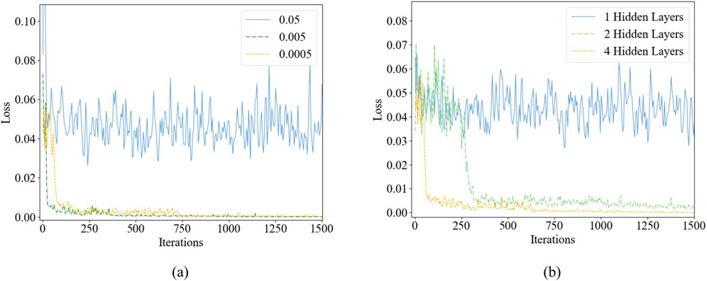
Figure 7. Training loss varies with different hyperparameters: (a) Different learning rates; (b) Different number of hidden layers.

Figure 8

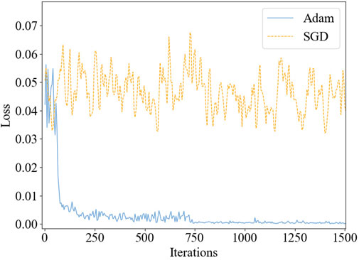
Figure 8. Training loss varies with different optimizers.

As the learning rate decreases, the model loss decreases. When the learning rates are set to 0.005 and 0.0005, the losses are similar, but the model accuracy is higher at a learning rate of 0.0005. Furthermore, when comparing different activation functions, Adam significantly outperforms SGD. The effect of varying the number of hidden layers was tested, and by comparing the loss to actual results, it was determined that a configuration with four hidden layers yields the best performance. Finally, Table 2 displays the CGAN model’s network framework configuration, with the detailed configuration parameters provided in Table 3.

Table 2

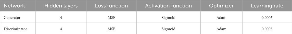
Table 2. CGAN’s network architecture and training parameter configurations.

Table 3

Table 3. Development environment.

To evaluate the predictive accuracy of the CGAN network, the classical infinite-length rigid cylinder model was selected as the benchmark. By splitting the data, a portion is selected as the test set, while the remaining data is used as the training set for training. The total number of sound pressure and sensitivity data is 401, with 10% of the dataset (i.e., 40 data points) selected as the test set, and the remaining data used as the training set. Figure 9a presents the sound pressure prediction results on the test dataset, while Figure 9b provides a comparative analysis of sensitivity predictions on the test dataset. In this context, Unknown Conditions refers to the test set, as the data patterns in the test set are unknown to the trained model. The results demonstrate that the CGAN model consistently achieves a high level of agreement with analytical solutions in both sound pressure predictions and sensitivity analyses. This indicates that the CGAN model effectively captures the underlying patterns within the data, even under unknown operating conditions, showcasing exceptional predictive accuracy and reliability. In addition, the sound pressure sensitivities were calculated using both the DBEM method and the CGAN model, with the results compared to the analytical solution, as shown in Figure 10. The figure clearly demonstrates that the CGAN model significantly outperforms the DBEM method in terms of accuracy, producing predictions that exhibit neither oscillatory behavior nor spurious frequency points. Furthermore, the CGAN model offers a substantial advantage in computational efficiency over the DBEM method. A detailed comparison of the results and corresponding computation times is provided in Tables 4, 5.

Figure 9

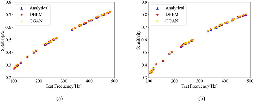
Figure 9. Comparison of CGAN Prediction Results Under Unknown Conditions (Training set:361, Test set: 40): (a) Sound Pressure; (b) Sensitivity.

Figure 10

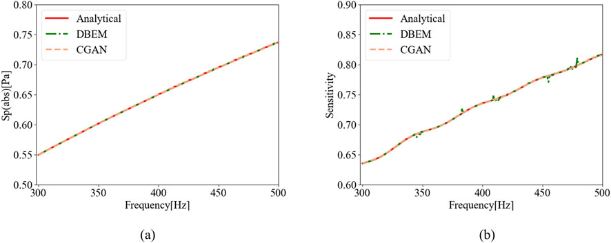
Figure 10. Comparison Between CGAN and DBEM(Training set:361, Test set: 40): (a) Sound Pressure; (b) Sensitivity.

Table 4

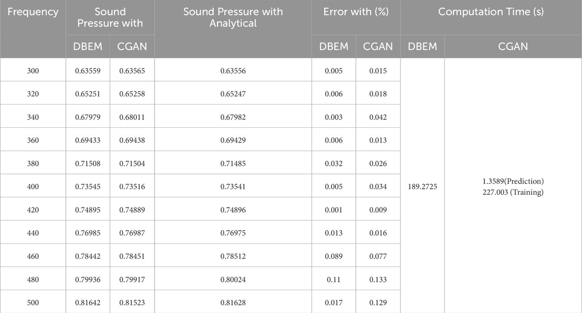
Table 4. Comparison of DBEM and CGAN results across different Frequencies (Sound pressure).

Table 5

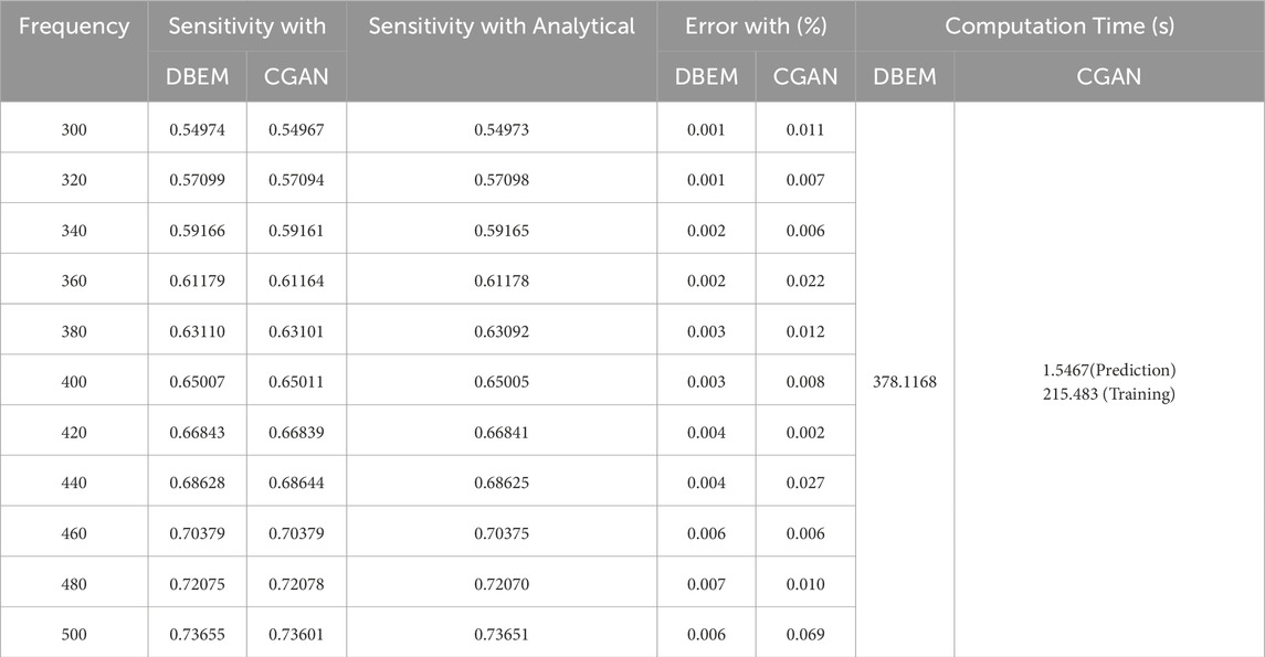
Table 5. Comparison of DBEM and CGAN results across different Frequencies (Sensitivity).

The data in the table indicate that DBEM and CGAN exhibit similar error performance. While DBEM demonstrates a slight edge in accuracy, CGAN significantly surpasses DBEM in computational time, achieving a notable reduction in the time required. This underscores the clear superiority of CGAN in computational efficiency. Thus, despite the minimal difference in error, CGAN offers a substantial advantage in time efficiency, making it the preferred choice for applications where computational speed is paramount.

4.2 Sound barrier model

As urbanization accelerates and the use of transportation vehicles becomes more widespread, traffic noise has become an increasingly severe issue, causing numerous inconveniences and hazards to people’s daily lives and work. Consequently, mitigating the harm caused by traffic noise is essential. Sound barriers are widely used in acoustic and noise control engineering as structures or devices designed to block or reduce the transmission of sound waves.

To evaluate the effectiveness of sound barriers, the accuracy and efficiency of the CGAN model were first validated using the infinitely long rigid cylinder model. In this section, a more complex noise barrier model is considered to comprehensively assess the CGAN model’s performance in terms of both precision and computational efficiency. The sound pressure and related data are generated from a plane wave incident parallel to the x-axis, which is scattered by the sound barrier. The sound barrier model is discretized into 1,118 elements, and the sound pressure at the point (12 m, 2 m) is calculated using the DBEM. From the obtained sound pressure and sensitivity data, the frequency range of 100—500 Hz is selected as the training dataset for the CGAN model. The sound barrier model is illustrated in Figure 11.

Figure 11

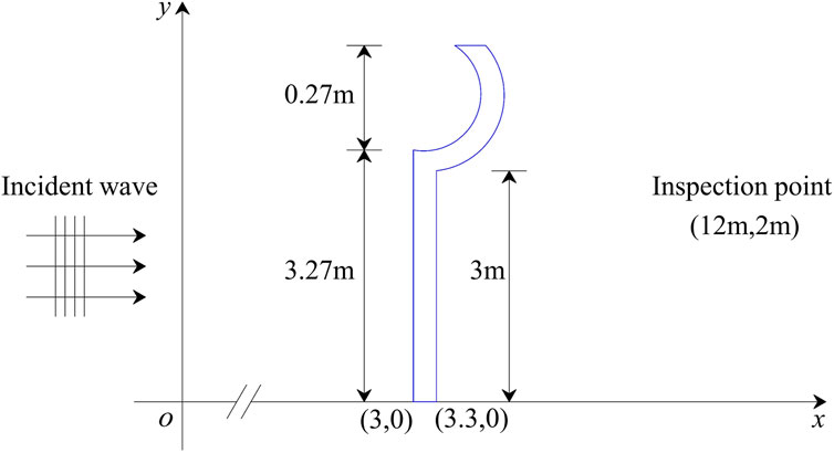
Figure 11. The design domain of the semi-curved sound barrier model.

The data processing method and the relative error calculation are consistent with those used in the infinitely long rigid cylinder model. The prediction results on the predefined test set are shown in Figure 12. As illustrated in the figure, the sound pressure and sensitivity predicted by the CGAN model exhibit the high degrees of consistency with the actual data, demonstrating excellent agreement. These findings highlight the generalization capability of the CGAN model when applied to unseen datasets. Furthermore, a comparative analysis between DBEM and CGAN was conducted within the frequency range of 200—400 Hz, with the results presented in Figure 13.

Figure 12

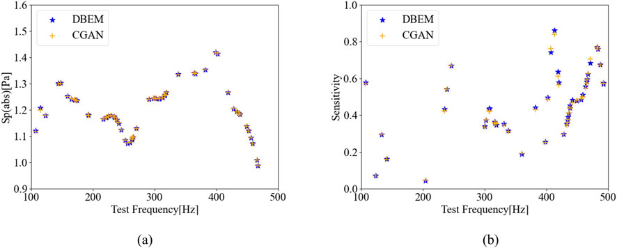
Figure 12. Comparison of CGAN’s Prediction Results on the Test Set with DBEM Results (Training set:361, Test set: 40): (a) Sound Pressure; (b) Sensitivity.

Figure 13

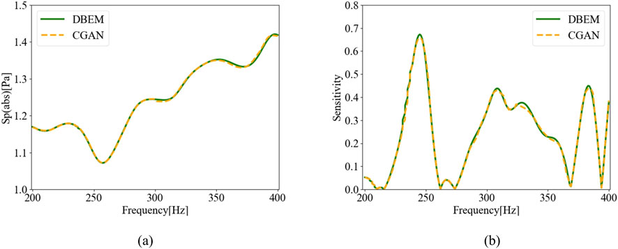
Figure 13. Comparison of CGAN’s Prediction Results with DBEM Results (Training set:361, Test set: 40): (a) Sound Pressure; (b) Sensitivity.

Table 6 presents the relative errors for several test points. It can be observed that all relative errors fall within a narrow range, with the maximum error not exceeding 3.62%. Unlike the infinite-length rigid cylinder model, the sound barrier model lacks analytical solutions and features more complex geometrical configurations. As a result, both DBEM and CGAN exhibit certain deviations. Nevertheless, the overall error remains within a small range, further validating the CGAN model’s ability to accurately learn patterns embedded in the data and deliver high-precision predictions.

Table 6

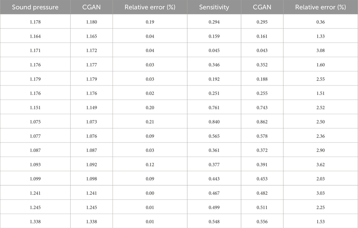
Table 6. CGAN testing input parameters and results.

In particular, the CGAN model demonstrates exceptional consistency and accuracy in sound pressure predictions. Figure 14 illustrates the relative error between the predicted values of the CGAN model and the calculated values of DBEM under different model configurations. For sensitivity predictions, although the data is inherently more complex and exhibits slightly higher errors compared to sound pressure, the CGAN model still maintains remarkably high prediction accuracy. This highlights the model’s capability to handle diverse data types while demonstrating robust performance and reliability. The regression model evaluation metrics were calculated using the specified formula, and the detailed statistical results are presented in Table 7.

Figure 14

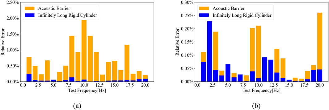
Figure 14. The relative errors between DBEM and CGAN under different models: (a) Sound pressure; (b) Sensitivity.

Table 7

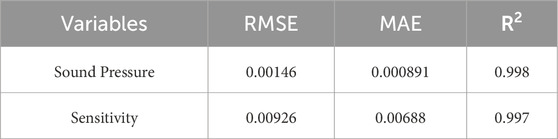
Table 7. Development environment.

Overall, these results comprehensively highlight the CGAN model’s outstanding capabilities and exceptional performance in sound barrier data prediction, reaffirming its effectiveness in addressing complex computational challenges. In the face of more complex models in the future, DBEM will require more time. The accuracy of the CGAN model has been demonstrated through the numerical example. Therefore, when calculating other models, it is sufficient to use the DBEM method to compute a portion of the data, and the remaining data can be generated using CGAN, which significantly reduces the computation time compared to the DBEM method.

5 Conclusion

This paper proposes a method to enhance computational efficiency by utilizing the CGAN network for the rapid and accurate prediction of sound pressure and sensitivity:

1. The integration of the Boundary Element Method (BEM) with CGAN is investigated to evaluate the applicability of CGAN in solving such problems.

2. The predictive model developed through CGAN demonstrates a significant reduction in computation time, thereby improving the efficiency of sound scattering analysis.

3. Adjustments to specific parameters and structures of CGAN have proven effective in addressing the regression challenges were encountered in this study.

Future research will aim to extend the application of CGAN to the structural optimization of sound barriers.

Data availability statement

The raw data supporting the conclusions of this article will be made available by the authors, without undue reservation.

Author contributions

QH: Conceptualization, Funding acquisition, Methodology, Software, Writing–review and editing. ZC: Data curation, Methodology, Software, Writing–original draft. HL: Data curation, Methodology, Software, Writing–original draft. SZ: Conceptualization, Methodology, Software, Supervision, Writing–original draft.

Funding

The author(s) declare that financial support was received for the research, authorship, and/or publication of this article. The authors appreciate the financial support of the Henan Provincial Department of Science and TechnologyResearch Project (No.222102230113).

Conflict of interest

The authors declare that the research was conducted in the absence of any commercial or financial relationships that could be construed as a potential conflict of interest.

Generative AI statement

The author(s) declare that no Generative AI was used in the creation of this manuscript.

Publisher’s note

All claims expressed in this article are solely those of the authors and do not necessarily represent those of their affiliated organizations, or those of the publisher, the editors and the reviewers. Any product that may be evaluated in this article, or claim that may be made by its manufacturer, is not guaranteed or endorsed by the publisher.

References

1. Chen L, Lian H, Pei Q, Meng Z, Jiang S, Dong H-W, et al. Fem-bem analysis of acoustic interaction with submerged thin-shell structures under seabed reflection conditions. Ocean Eng (2024) 309:118554. doi:10.1016/j.oceaneng.2024.118554

CrossRef Full Text | Google Scholar

2. Xu Y, Yang S. Sensitivity analysis of non-uniform rational b-splines–based finite element/boundary element coupling in structural-acoustic design. Front Phys (2024) 12:1428875. doi:10.3389/fphy.2024.1428875

CrossRef Full Text | Google Scholar

3. Chen L, Lian H, Xu Y, Li S, Liu Z, Atroshchenko E, et al. Generalized isogeometric boundary element method for uncertainty analysis of time-harmonic wave propagation in infinite domains. Appl Math Model (2023) 114:360–78. doi:10.1016/j.apm.2022.09.030

CrossRef Full Text | Google Scholar

4. Vuong CD, Yu T, Rungamornrat J, Bui TQ. A smoothing gradient thermo-mechanical damage model for thermal shock crack propagation: theory and fe implementation. Int J Non-Linear Mech (2024) 163:104755. doi:10.1016/j.ijnonlinmec.2024.104755

CrossRef Full Text | Google Scholar

5. Mahrous E, Valéry Roy R, Jarauta A, Secanell M. A three-dimensional numerical model for the motion of liquid drops by the particle finite element method. Phys Fluids (2022) 34. doi:10.1063/5.0091699

CrossRef Full Text | Google Scholar

6. Liu Z, Sheng L, Liu X, Chang Y, Chen G, Guo X. Mechanical analysis for deepwater drilling riser system with structural parameters uncertainty. Ocean Eng (2024) 305:118049. doi:10.1016/j.oceaneng.2024.118049

CrossRef Full Text | Google Scholar

7. Chen L, Liu C, Lian H, Gu W. Electromagnetic scattering sensitivity analysis for perfectly conducting objects in tm polarization with isogeometric bem. Eng Anal Boundary Elem (2025) 172:106126. doi:10.1016/j.enganabound.2025.106126

CrossRef Full Text | Google Scholar

8. Liu C, Pei Q, Cui Z, Song Z, Zhao G, Yang Y. Isogeometric boundary element method analysis for dielectric target shape optimization in electromagnetic scattering. Sci Prog (2024) 107:00368504241294114. doi:10.1177/00368504241294114

PubMed Abstract | CrossRef Full Text | Google Scholar

9. Padrino JC, Sprittles JE, Lockerby DA. Efficient simulation of rarefied gas flow past a particle: a boundary element method for the linearized g13 equations. Phys Fluids (2022) 34. doi:10.1063/5.0091041

CrossRef Full Text | Google Scholar

10. Langins A, Stikuts AP, Cēbers A. A three-dimensional boundary element method algorithm for simulations of magnetic fluid droplet dynamics. Phys Fluids (2022) 34. doi:10.1063/5.0092532

CrossRef Full Text | Google Scholar

11. Chen L, Lian H, Liu Z, Chen H, Atroshchenko E, Bordas S. Structural shape optimization of three dimensional acoustic problems with isogeometric boundary element methods. Computer Methods Appl Mech Eng (2019) 355:926–51. doi:10.1016/j.cma.2019.06.012

CrossRef Full Text | Google Scholar

12. [Dataset] Zhong S, Jiang X, Du J, Liu J. A reduced-order boundary element method for two-dimensional acoustic scattering. Front Phys (2024) 12. doi:10.3389/fphy.2024.1464716

CrossRef Full Text | Google Scholar

13. Marburg S. Six boundary elements per wavelength: is that enough? J Comput Acoust (2002) 10:25–51. doi:10.1142/s0218396x02001401

CrossRef Full Text | Google Scholar

14. Marburg S, Schneider S. Influence of element types on numeric error for acoustic boundary elements. J Comput Acoust (2003) 11:363–86. doi:10.1142/s0218396x03001985

CrossRef Full Text | Google Scholar

15. Arnold S (1949). Partial differential equations in physics

Google Scholar

16. Sobolev A. Wide-band sound-absorbing structures for aircraft engine ducts. Acoust Phys (2000) 46:466–73. doi:10.1134/1.29911

CrossRef Full Text | Google Scholar

17. Willmann E, Boll B, Mikaelyan G, Wittich H, Meißner RH, Fiedler B. Vibro-acoustic modulation based measurements in cfrp laminates for damage detection in open-hole structures. Composites Commun (2023) 42:101659. doi:10.1016/j.coco.2023.101659

CrossRef Full Text | Google Scholar

18. Xiao Q, Zhang G, Chen Z, Wu G, Xu Y. A hybrid csrpim/sea method for the analysis of vibro-acoustic problems in mid-frequency range. Eng Anal Boundary Elem (2023) 146:146–54. doi:10.1016/j.enganabound.2022.10.004

CrossRef Full Text | Google Scholar

19. Zhao K, Li H, Zha Z, Zhai M, Wu J. Detection of sub-healthy apples with moldy core using deep-shallow learning for vibro-acoustic multi-domain features. Meas Food (2022) 8:100068. doi:10.1016/j.meafoo.2022.100068

CrossRef Full Text | Google Scholar

20. Chen L, Huo R, Lian H, Yu B, Zhang M, Natarajan S, et al. Uncertainty quantification of 3d acoustic shape sensitivities with generalized nth-order perturbation boundary element methods. Computer Methods Appl Mech Eng (2025) 433:117464. doi:10.1016/j.cma.2024.117464

CrossRef Full Text | Google Scholar

21. Chen L, Lian H, Liu C, Li Y, Natarajan S. Sensitivity analysis of transverse electric polarized electromagnetic scattering with isogeometric boundary elements accelerated by a fast multipole method. Appl Math Model (2025) 141:115956. doi:10.1016/j.apm.2025.115956

CrossRef Full Text | Google Scholar

22. Chen L, Pei Q, Fei Z, Zhou Z, Hu Z. Deep-neural-network-based framework for the accelerating uncertainty quantification of a structural–acoustic fully coupled system in a shallow sea. Eng Anal Boundary Elem (2025) 171:106112. doi:10.1016/j.enganabound.2024.106112

CrossRef Full Text | Google Scholar

23. Biancoli A, Fancher CM, Jones JL, Damjanovic D. Breaking of macroscopic centric symmetry in paraelectric phases of ferroelectric materials and implications for flexoelectricity. Nat Mater (2015) 14:224–9. doi:10.1038/nmat4139

PubMed Abstract | CrossRef Full Text | Google Scholar

24. Wang C, Hong L, Qiang X, Xu M. Novel numerical method for uncertainty analysis of coupled vibro-acoustic problem considering thermal stress. Computer Methods Appl Mech Eng (2024) 420:116727. doi:10.1016/j.cma.2023.116727

CrossRef Full Text | Google Scholar

25. Lian H, Li X, Qu Y, Du J, Meng Z, Liu J, et al. Bayesian uncertainty analysis for underwater 3d reconstruction with neural radiance fields. Appl Math Model (2024) 138:115806. doi:10.1016/j.apm.2024.115806

CrossRef Full Text | Google Scholar

26. Jiang S, Liang Y, Cheng Y, Gao L. Research on the prediction method of wing structure noise based on the combination of conditional generative adversarial neural network and numerical methods. Front Phys (2024) 12:1452876. doi:10.3389/fphy.2024.1452876

CrossRef Full Text | Google Scholar

27. Chen L, Cheng R, Li S, Lian H, Zheng C, Bordas SP. A sample-efficient deep learning method for multivariate uncertainty qualification of acoustic–vibration interaction problems. Computer Methods Appl Mech Eng (2022) 393:114784. doi:10.1016/j.cma.2022.114784

CrossRef Full Text | Google Scholar

28. Carazo A, Roger M, Omais M. Analytical prediction of wake-interaction noise in counter-rotating open rotors. In: 17th AIAA/CEAS aeroacoustics conference (32nd AIAA aeroacoustics conference) (2011). p. 2758.

Google Scholar

29. Samaniego E, Anitescu C, Goswami S, Nguyen-Thanh VM, Guo H, Hamdia K, et al. An energy approach to the solution of partial differential equations in computational mechanics via machine learning: concepts, implementation and applications. Computer Methods Appl Mech Eng (2020) 362:112790. doi:10.1016/j.cma.2019.112790

CrossRef Full Text | Google Scholar

30. Zhang J, Zhang W, Zhu J, Xia L. Integrated layout design of multi-component systems using xfem and analytical sensitivity analysis. Computer Methods Appl Mech Eng (2012) 245:75–89. doi:10.1016/j.cma.2012.06.022

CrossRef Full Text | Google Scholar

31. Dühring MB, Jensen JS, Sigmund O. Acoustic design by topology optimization. J sound vibration (2008) 317:557–75. doi:10.1016/j.jsv.2008.03.042

CrossRef Full Text | Google Scholar

32. Chen L, Lu C, Lian H, Liu Z, Zhao W, Li S, et al. Acoustic topology optimization of sound absorbing materials directly from subdivision surfaces with isogeometric boundary element methods. Computer Methods Appl Mech Eng (2020) 362:112806. doi:10.1016/j.cma.2019.112806

CrossRef Full Text | Google Scholar

33. Hombal V, Mahadevan S. Bias minimization in Gaussian process surrogate modeling for uncertainty quantification. Visualization Mech Process An Int Online J (2011) 1:321–49. doi:10.1615/int.j.uncertaintyquantification.2011003343

CrossRef Full Text | Google Scholar

34. Olofsson S, Deisenroth MP, Misener R. Design of experiments for model discrimination using Gaussian process surrogate models. Computer Aided Chem Eng (Elsevier) (2018) 44:847–52. doi:10.1016/B978-0-444-64241-7.50136-1

CrossRef Full Text | Google Scholar

35. Li MY, Grant E, Griffiths TL. Gaussian process surrogate models for neural networks. Uncertainty Artif Intelligence (Pmlr) (2023) 1241–52.

Google Scholar

36. Bilionis I, Zabaras N. Multidimensional adaptive relevance vector machines for uncertainty quantification. SIAM J Scientific Comput (2012) 34:B881–B908. doi:10.1137/120861345

CrossRef Full Text | Google Scholar

37. Chen L, Zhao J, Lian H, Yu B, Atroshchenko E, Li P. A bem broadband topology optimization strategy based on taylor expansion and soar method-application to 2d acoustic scattering problems. Int J Numer Methods Eng (2023) 124:5151–82. doi:10.1002/nme.7345

CrossRef Full Text | Google Scholar

38. Lakshminarayanan B, Pritzel A, Blundell C. Simple and scalable predictive uncertainty estimation using deep ensembles. Adv Neural Inf Process Syst (2017) 30.

Google Scholar

39. Sriboriboon P, Qiao H, Kwon O, Vasudevan RK, Jesse S, Kim Y. Deep learning for exploring ultra-thin ferroelectrics with highly improved sensitivity of piezoresponse force microscopy. npj Comput Mater (2023) 9:28. doi:10.1038/s41524-023-00982-0

CrossRef Full Text | Google Scholar

40. He J, Wang C, Li J, Liu C, Xue D, Cao J, et al. Machine learning assisted prediction of dielectric temperature spectrum of ferroelectrics. J Adv Ceramics (2023) 12:1793–804. doi:10.26599/jac.2023.9220788

CrossRef Full Text | Google Scholar

41. Wang Y, Liao Z, Shi S, Wang Z, Poh LH. Data-driven structural design optimization for petal-shaped auxetics using isogeometric analysis. Computer Model Eng and Sci (2020) 122:433–58. doi:10.32604/cmes.2020.08680

CrossRef Full Text | Google Scholar

42. Oishi A, Yagawa G. Computational mechanics enhanced by deep learning. Computer Methods Appl Mech Eng (2017) 327:327–51. doi:10.1016/j.cma.2017.08.040

CrossRef Full Text | Google Scholar

43. Chen L, Wang Z, Lian H, Ma Y, Meng Z, Li P, et al. Reduced order isogeometric boundary element methods for cad-integrated shape optimization in electromagnetic scattering. Computer Methods Appl Mech Eng (2024) 419:116654. doi:10.1016/j.cma.2023.116654

CrossRef Full Text | Google Scholar

44. Levine Y, Wies N, Sharir O, Cohen N, Shashua A. Tensors for deep learning theory: analyzing deep learning architectures via tensorization. In: Tensors for data processing. Elsevier (2022). p. 215–48.

Google Scholar

45. Huang G, Wu G, Yang Z, Chen X, Wei W. Development of surrogate models for evaluating energy transfer quality of high-speed railway pantograph-catenary system using physics-based model and machine learning. Appl Energy (2023) 333:120608. doi:10.1016/j.apenergy.2022.120608

CrossRef Full Text | Google Scholar

46. Chen L, Lian H, Natarajan S, Zhao W, Chen X, Bordas S. Multi-frequency acoustic topology optimization of sound-absorption materials with isogeometric boundary element methods accelerated by frequency-decoupling and model order reduction techniques. Computer Methods Appl Mech Eng (2022) 395:114997. doi:10.1016/j.cma.2022.114997

CrossRef Full Text | Google Scholar

47. Zhou Z, Gao Y, Cheng Y, Ma Y, Wen X, Sun P, et al. Uncertainty quantification of vibroacoustics with deep neural networks and catmull–clark subdivision surfaces. Shock and Vibration (2024) 2024:7926619. doi:10.1155/2024/7926619

CrossRef Full Text | Google Scholar

48. Chen L, Lian H, Liu Z, Gong Y, Zheng C, Bordas S. Bi-material topology optimization for fully coupled structural-acoustic systems with isogeometric fem–bem. Eng Anal Boundary Elem (2022) 135:182–95. doi:10.1016/j.enganabound.2021.11.005

CrossRef Full Text | Google Scholar

49. Stam J. Exact evaluation of catmull-clark subdivision surfaces at arbitrary parameter values. Seminal Graphics Pap Pushing Boundaries (2023) 2:139–48. doi:10.1145/3596711.3596728

CrossRef Full Text | Google Scholar

50. Qu Y, Zhou Z, Chen L, Lian H, Li X, Hu Z, et al. Uncertainty quantification of vibro-acoustic coupling problems for robotic manta ray models based on deep learning. Ocean Eng (2024) 299:117388. doi:10.1016/j.oceaneng.2024.117388

CrossRef Full Text | Google Scholar

51. Chen L, Lian H, Dong H-W, Yu P, Jiang S, Bordas SP. Broadband topology optimization of three-dimensional structural-acoustic interaction with reduced order isogeometric fem/bem. J Comput Phys (2024) 509:113051. doi:10.1016/j.jcp.2024.113051

CrossRef Full Text | Google Scholar

52. Wang S, Cao J, Philip SY. Deep learning for spatio-temporal data mining: a survey. IEEE Trans knowledge Data Eng (2020) 34:3681–700. doi:10.1109/TKDE.2020.3025580

CrossRef Full Text | Google Scholar

53. Burton A, Miller G. The application of integral equation methods to the numerical solution of some exterior boundary-value problems. Proc R Soc Lond A. Math Phys Sci (1971) 323:201–10. doi:10.1098/rspa.1971.0097

CrossRef Full Text | Google Scholar

54. Gauthier J. Conditional generative adversarial nets for convolutional face generation. 2 (2014).Class project Stanford CS231N: convolutional Neural networks Vis recognition

Google Scholar

55. Mirza M. Conditional generative adversarial nets. arXiv preprint arXiv:1411.1784 (2014). doi:10.48550/arXiv.1411.1784

CrossRef Full Text | Google Scholar