Training networks without wavefront label for pixel-based wavefront sensing

Traditional image-based wavefront sensing often faces challenges in efficiency and stagnation. Deep learning methods, when properly trained, offer superior robustness and performance. However, obtaining sufficient real labeled data remains a significant challenge. Existing self-supervised methods based on Zernike coefficients struggle to resolve high-frequency phase components. To solve this problem, this paper proposes a pixel-based self-supervised learning method for deep learning wavefront sensing. This method predicts the wavefront aberration in pixel dimensions and preserves more high-frequency information while ensuring phase continuity by adding phase constraints. Experiments show that the network can accurately predict the wavefront aberration on a real dataset, with a root mean square error of 0.017λ. resulting in a higher detection accuracy compared with the method of predicting the aberration with Zernike coefficients. This work contributes to the application of deep learning to high-precision image-based wavefront sensing in practical conditions.

1 Introduction

Traditional image-based wavefront sensing methods, including model-based approach, phase retrieval (PR), and phase diversity (PD), etc., have been widely applied in the areas of adaptive and active optics [1], microscopy imaging [2], and laser technologies [3]. Compared to other wavefront sensing methods (Hartmann sensor [4, 5] or shearing interferometry [6]), it has lower optical hardware requirements and does not require additional calibration [7]. The model-based approach leverages predefined aberration modes and typically requires only a single iteration [8–10], resulting in a faster convergence rate. However, its execution cost is significantly greater, and its convergence accuracy is limited because it only has one iteration [11, 12]. On the other hand, iterative methods like PR and PD achieve higher accuracy by refining the solution over multiple iterations. Nevertheless, as these methods involve solving a non-convex optimization problem, they are prone to stagnation during the iterative process, compromising their robustness. Furthermore, the iterative nature of these methods makes it challenging to optimize their computational efficiency using parallel computing platforms, such as GPUs or FPGAs [13]. These challenges pose substantial barriers to the widespread adoption and application of image-based wavefront sensing technologies.

Deep learning networks have been introduced to image-based wavefront sensing for many applications [14–17] due to their superiorities in efficiency and robustness. The network predicts the wavefront aberration based on the input point spread function (PSF). Depending on the representation of the wavefront aberration, it can be categorized into Zernike-based and pixel-based methods. The Zernike-based method reconstructs the wavefront from the Zernike coefficients predicted by the network. Ju et al. [12] represent the features of PSFs in terms of Tchebichef moments and input them to a multilayer perceptron (MLP) network. This method reduces the complexity of the network while maintaining a comparatively high accuracy. Qi et al. [18] use both in-focus and out-of-focus PSFs to generate object-independent features as inputs to the long short-term memory (LSTM) network for arbitrary objects, and the network achieves comparable accuracy to the phase diversity (PD) algorithm when predicting the 9-term Zernike coefficients. Zhou et al. [19, 20] introduced a generalized Fourier-based phase diversity wavefront sensing method. This approach accommodates arbitrary objects and allows direct application to new systems without additional training, even when the system parameters are altered. Ge et al. [21] use a convolutional neural network (CNN) to predict the wavefront aberration coefficients based on PSFs and analyze the change in accuracy as the network outputs with different coefficient orders. Abu et al. [22] demonstrate the ambiguity that exists between the sign of the Zernike coefficients and the PSF when using a single PSF to predict wavefront aberrations and modify the Zernike polynomials to remove this ambiguity.

For pixel-based wavefront sensing methods, the network directly outputs pixel-dimensional wavefront aberrations that can contain more high-frequency components than Zernike-based methods [23]. Zhuang et al. [24] employ a fully connected retrieval neural network (F-RNN) to directly predict wavefront aberrations. They enhance network performance by extracting and integrating multi-scale feature maps from various layers and stages through fully-skip cross-connections. In addressing complex wavefronts, Hu et al. [25] not only use the network to predict Zernike coefficients but also employ an additional network that utilizes these coefficients to predict wavefront aberrations on a pixel-by-pixel basis further. Agarwal et al. [26] introduce cGULnet to directly generate wavefront aberrations in scenarios with high turbulence, training it using a generative adversarial network approach. Jeffrey et al. [27] utilize U-Net to accurately represent fine details in the phase, ensuring precise reconstruction of the PSF. Zhao et al. [28] concentrate on the impact of network models on detection accuracy. They enhance U-Net by incorporating a Dense Block and Attention Gates structure, further improving its accuracy in directly predicting wavefront aberrations.

However, supervised training requires prior knowledge of the true wavefront corresponding to the input PSF, referred to as the wavefront label. In some practical applications, acquiring a large number of real PSF images with their corresponding wavefront labels can be challenging. Although a large number of images and corresponding labels can be obtained through simulation, there are inevitable differences between simulated and actual images. This leads to poor model performance in the real case, as shown in Figures 1B, C (The true value is shown in Figure 1A and the root mean square error (RMSE) between each prediction and the true value is marked above the wavefront maps).

Figure 1

Figure 1. Comparison of results of different methods. (A) truth value. (B–E) show the predicted wavefront using the supervised Zernike-based method, supervised pixel-based method, self-supervised Zernike-based method, and self-supervised pixel-based method, respectively. (F) the self-supervised pixel-based method proposed in this paper. The RMSE between each predicted result and the true value, as well as the RMSE for the C5-C9 terms, are marked above the corresponding wavefront maps.

Self-supervised learning allows the model to learn from unlabeled data by leveraging inherent data structures or constraints. In wavefront sensing, the PSF has a well-defined mathematical relationship with the wavefront label, which can serve as a constraint in self-supervised training. Several self-supervised training methods [29–31] for point and arbitrary objects have been proposed, all of which utilize Zernike polynomials to represent the wavefront to ensure phase continuity. However, fitting the high-frequency components with Zernike coefficients is difficult and leads to poor results when there is more high-frequency information in the wavefront, as shown in Figure 1D. Whereas, if the wavefront is output directly in the pixel dimension in the self-supervised method, it results in an erroneous, discontinuous wavefront, as shown in Figure 1E.

To solve the above problems, this paper introduces a new self-supervised deep learning method for pixel-based high-precision wavefront sensing, and the result is shown in Figure 1F. The method operates without the need for wavefront labels and eliminates the use of Zernike polynomials to represent the wavefront phase map. It can predict wavefront aberrations in the pixel dimension while guaranteeing phase continuity. In particular, the network output is divided into two components: the main part capturing the low-frequency component of the wavefront distortion to ensure phase continuity and the high-frequency component used for predicting detailed wavefront information. The final wavefront prediction is achieved by combining these two components while ensuring wavefront continuity.

2 Materials and methods

2.1 Basic theory

For an incoherent imaging system, the image at the $i$-th image plane of the system can be represented as a convolution of the object and the PSF of the system, as expressed in Equation 1

$d_i\left(\mathit{r}\right)=o\left(\mathit{r}\right)*h_i\left(\mathit{r}\right)+n_i\left(\mathit{r}\right)(1)$

where $d_i\left(\mathit{r}\right)$ is the corresponding light intensity distribution on the $i$-th image plane, $o\left(\mathit{r}\right)$ is the object, $h_i\left(\mathit{r}\right)$ is the PSF on the corresponding image plane, $n_i\left(\mathit{r}\right)$ is the noise, $*$ denotes the convolution operation, and $\mathit{r}$ is a two-dimensional position vector on the image plane. Further, the PSF of the system can be expressed as:

$h_i\left(\mathit{r}\right)={\left|\mathcal{F}\left\{A\left(\mathit{\rho }\right)\cdot e^{j{\phi }_i\left(\mathit{\rho }\right)}\right\}\right|}^2(2)$

where $A\left(\mathit{\rho }\right)$ is the optical pupil amplitude, ${\phi }_i\left(\mathit{\rho }\right)$ is the wavefront aberration, $\mathit{\rho }$ is the 2D position vector on the optical pupil plane, and $\mathcal{F}$ denotes the 2D Fourier transform. For different image planes at different positions, the wavefront aberration can be represented as Equation 3:

${\phi }_i\left(\mathit{\rho }\right)=\phi \left(\mathit{\rho }\right)+{∆}_i\left(\mathit{\rho }\right)(3)$

where $\phi \left(\mathit{\rho }\right)$ is the aberration that is unknown and needs to be solved for, and ${∆}_i\left(\mathit{\rho }\right)$ is the wave aberration determined by the known image plane position (e.g., defocus terms in Zernike coefficients). During the imaging process of a real optical system, it is inevitable that it will be interfered with by surface shape errors, airflow, and so on. These interferences introduce high-frequency components into $\phi \left(\mathit{\rho }\right)$, so $\phi \left(\mathit{\rho }\right)$ can be further divided into high-frequency and low-frequency components [32],

$\phi \left(\mathit{\rho }\right)={\phi }_l\left(\mathit{\rho }\right)+{\phi }_h\left(\mathit{\rho }\right)(4)$

where ${\phi }_l\left(\mathit{\rho }\right)$ and ${\phi }_h\left(\mathit{\rho }\right)$ denote the low-frequency and high-frequency components that need to be solved, respectively.

2.2 Overall framework

The overall framework of the proposed method is shown in Figure 2A. In the training phase, the network inputs are PSFs collected from a real optical system. Concerning Equation 4, the output wavefront distribution of the network is split into high and low frequencies using low-pass and high-pass filters at specific frequencies. The final network prediction is then derived by weighting and combining these two separate components. The estimated PSFs are then computed from the predicted wavefront aberrations employing an imaging model corresponding to the real optical system. Ultimately, the loss is calculated by comparing the estimated PSFs with the actual PSFs, which is used to optimize network parameters.

Figure 2

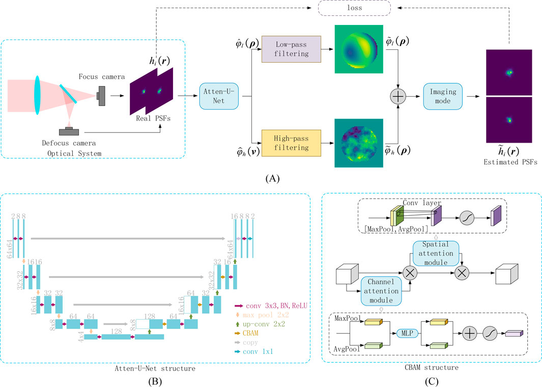
Figure 2. Structure of the proposed self-supervised deep learning method. (A) represents the overall structure, (B) is the structure of Atten-U-Net and (C) denotes the structure of CBAM.

2.3 Network structure

A modified U-Net architecture, termed Atten-U-Net, is employed for predicting wavefront aberrations, incorporating the Convolutional Block Attention Module (CBAM) as the attention mechanism [33, 34]. The network structure is depicted in Figure 2B, with both input and output image spatial dimensions set at 64 × 64. Intermediate feature maps’ spatial and channel dimensions are annotated on the left and top, respectively.

The Atten-U-Net consists of two main phases: encoding and decoding. In the encoding phase, the feature map undergoes two consecutive basic modules comprising 3 × 3 convolution, Batch Normalization (BN), and Rectified Linear Unit (ReLU). Subsequently, downsampling occurs through a Maxpooling layer, reducing spatial dimensions and doubling channel dimensions to extract higher-dimensional semantic information.

During the decoding stage, spatial dimensions of the features are expanded, and channel dimensions are reduced through transposed convolution. These features are then concatenated with corresponding feature maps from the encoding phase to reintegrate missing detail information. CBAM is applied to fuse features before being output to the subsequent layer.

The CBAM structure, illustrated in Figure 2C, concurrently enhances features in spatial and channel dimensions. It comprises two modules: the channel attention module and the spatial attention module. In the former, the input spatial dimension of the features is compressed to one dimension through Maxpooling and Avgpooling layers, followed by processing through a MLP. The outputs are summed and multiplied with the original feature map in the channel dimension after the sigmoid function, enhancing the channel dimension. In the latter, the channel dimension of input features is compressed by Maxpooling and Avgpooling layers, fed into a 7 × 7 convolution, and the result is multiplied with the original features in the spatial dimension after a sigmoid function, augmenting the spatial dimension.

2.4 Restrictive condition

First, a low-pass filter is used to suppress the high-frequency components of the network outputs. This allows the network to search for the correct solution that will make the wavefront continuous during training. The frequency domain filtering process can be expressed as:

${\stackrel{\sim }{\phi }}_l\left(\mathit{\rho }\right)={\mathcal{F}}^{-1}\left\{{\widehat{\mathit{\Phi }}}_l\left(\mathit{v}\right)\cdot LF\left(\mathit{v}\right)\right\}={\mathcal{F}}^{-1}\left\{\mathcal{F}\left\{{\widehat{\phi }}_l\left(\mathit{\rho }\right)\right\}\cdot LF\left(\mathit{v}\right)\right\}(5)$

where ${\widehat{\phi }}_l\left(\mathit{\rho }\right)$ is the wavefront output directly from the network, and ${\stackrel{\sim }{\phi }}_l\left(\mathit{\rho }\right)$ is the corresponding result after a low-pass filter. $\mathit{v}$ is a two-dimensional position vector in frequency space. $LF\left(\mathit{v}\right)$ is the spectrum of the filter, a Gaussian low-pass filter is employed which is given by Equation 6:

$LF\left(\mathit{v}\right)=e^{-\left(\frac{{\left|\mathit{v}\right|}^2}{2{r_l}^2}\right)}(6)$

where $r_l$ controls the radius of the filter and is a trainable parameter. Accordingly, to solve for the high-frequency components, a Butterworth high pass filter is employed which frequency response can be expressed as Equation 7:

$HF\left(\mathit{v}\right)=\frac{1}{1+{\left(r_h/\mathit{v}\right)}^{2n}}(7)$

The cutoff frequency of the filter is represented by $r_h$, while $n$ represents the order of the Butterworth filter. Similar to Equation 5, ${\stackrel{\sim }{\phi }}_h\left(\mathit{\rho }\right)$ can be calculated as:

${\stackrel{\sim }{\phi }}_h\left(\mathit{\rho }\right)={\mathcal{F}}^{-1}\left\{\mathcal{F}\left\{{\widehat{\phi }}_h\left(\mathit{\rho }\right)\right\}\cdot HF\left(\mathit{v}\right)\right\}(8)$

To prevent additional discontinuities when adding the result ${\stackrel{\sim }{\phi }}_l\left(\mathit{\rho }\right)$ of the low-frequency filtering to the result ${\stackrel{\sim }{\phi }}_h\left(\mathit{\rho }\right)$ of the high-frequency filtering, the maximum difference between neighboring values in the low-frequency component is first calculated as Equation 9:

$D_l=\underset{\mathit{\rho }}{\max }\left|{\stackrel{\sim }{\phi }}_l\left(\mathit{\rho }\right)-{\stackrel{\sim }{\phi }}_l\left(\mathit{\rho }+\mathit{d}\right)\right|(9)$

where $\mathit{d}$ is the direction vector which takes the values $\left(0,\pm 1\right)$, $\left(\pm 1,0\right)$ respectively. The prediction of the wavefront distortion is then obtained by limiting the maximum value of ${\stackrel{\sim }{\phi }}_h\left(\mathit{\rho }\right)$ by $D_l$ and then summing it with ${\stackrel{\sim }{\phi }}_l\left(\mathit{\rho }\right)$, as expressed in Equation 10:

$\stackrel{\sim }{\phi }\left(\mathit{\rho }\right)={\stackrel{\sim }{\phi }}_l\left(\mathit{\rho }\right)+\frac{2\pi -D_l}{2\max \left|{\stackrel{\sim }{\phi }}_h\left(\mathit{\rho }\right)\right|}{\stackrel{\sim }{\phi }}_h\left(\mathit{\rho }\right)(10)$

2.5 Imaging model and loss function

The PSF calculation for the ideal state has been given in Equation 2, but in reality, the actual optical system will inevitably be affected by micro-jitter during the imaging process. This micro-jitter between the image on the image plane and the image plane detector reduces the sensing resolution, thus presenting a Gaussian blur [35, 36]. Assuming that the horizontal and vertical jitter are independent of each other and that their means are 0 and the variances are $\sigma$, the estimated PSF after accounting for micro-jitter can be calculated as Equation 11:

${\stackrel{\sim }{h}}_i\left(\mathit{r}\right)={\left|\mathcal{F}\left\{A\left(\mathit{\rho }\right)\cdot e^{j\left[\stackrel{\sim }{\phi }\left(\mathit{\rho }\right)+{∆}_i\left(\mathit{\rho }\right)\right]}\right\}\right|}^2*\frac{1}{2\pi {\sigma }^2}{e}^{-\left(\frac{{\left|\mathit{r}\right|}^2}{2{\sigma }^2}\right)}(11)$

Note that for the deviation of the known position of the image plane from its actual position, the methods based on the Zernike fit need to additionally solve for the defocus and tilt terms to compensate for the effect of the error. Whereas in this paper, no additional compensation is required since the information about the entire wavefront is solved directly in pixel dimension, which automatically includes the defocus and tilt terms.

Smooth L1 loss [37] and structure similarity index measure (SSIM) loss [38] were used to measure the difference between the estimated PSFs and the real PSFs, and they were weighted by the constant $\beta$ to obtain the total loss $\mathcal{L}$, as expressed in Equation 12.

$\mathcal{L}={\displaystyle \sum _i}\beta {\mathcal{L}}_{smothL1}\left({\stackrel{\sim }{h}}_i\left(\mathit{r}\right),h_i\left(\mathit{r}\right)\right)+{\mathcal{L}}_{SSIM}\left({\stackrel{\sim }{h}}_i\left(\mathit{r}\right),h_i\left(\mathit{r}\right)\right)(12)$

3 Simulations

In this section, simulated images are used to demonstrate the accuracy of the proposed method. The wavefront aberration of the simulation experiment contains both simple and complex parts, as shown in Figure 3. The simple wavefront has a lower frequency. It is generated according to random Zernike’s C5-C21 terms. The complex wavefront has a higher frequency and is generated based on the airflow distribution [39]. The percentage of the two parts is adjusted by parameter $\alpha$. The wavefront labels are represented using Zernike coefficients and pixels respectively. Where the labels of Zernike coefficients are used to train supervised Zernike-based networks. The pixel dimension labels are used to train supervised pixel-based networks. The self-supervised networks are all trained by PSF only.

Figure 3

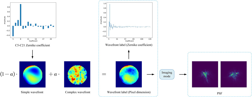
Figure 3. Schematic of simulated wavefront distortion and PSF generation.

The simulation experiments are verified in two main ways, i.e., wavefront aberration of different complexity and ranges. As shown in Table 1, 10 sets of data are generated. The first 5 datasets are generated by adjusting $\alpha$ and fixing PV = 1.0. the purpose is to validate the model under conditions with different levels of complexity of the aberration. The last 5 datasets are generated by fixing $\alpha$ = 0.250 and adjusting PV. The purpose is to validate the model under different ranges of aberration conditions.

Table 1

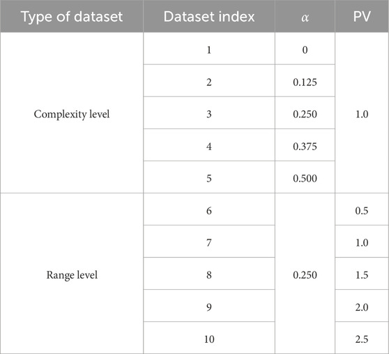
Table 1. Settings of the 10 simulation datasets.

For each dataset in Table 1, 10,000 pairs of training data and 1000 pairs of test data are generated. The PSF size was 64 × 64. The axial defocusing distance between each pair of PSFs (one PSF is obtained in front of the focus point and another is obtained behind the focus point) is 1.6mm, and a position error of each PSF in the range of [-0.1mm, 0.1 mm] is further imposed. 40dB Gaussian noise is added to each PSF. For the Zernike-based approaches, the ResNet-50 network is used (the same as Refs. [4, 40, 41]). A GeForce RTX 3060 graphics card was used to train the network using the Adam optimizer with a learning rate of 0.001 and weight delay of ${10}^{-6}$. The batch size for training was 32, the total epoch was 200, and the learning rate was halved every 40 epochs.

3.1 Impact of wavefront aberrations of different complexity on detection accuracy

In order to quantitatively analyze the performance of the different methods. The first five datasets in Table 1 are selected for training and testing, respectively. Figure 4 demonstrates the average RMSE of each method on different datasets. The following three conclusions can be drawn from Figure 4:

(1) On all datasets, pixel-based methods outperform the Zernike-based methods when the training methods are the same.

(2) The supervised method outperforms the self-supervised method on all datasets.

(3) In self-supervised methods, when the wavefront is simple, the performance difference between pixel-based and Zernike-based methods is not significant. The more complex the wavefront is, the better the performance of the pixel-based method than the Zernike-based method.

Figure 4

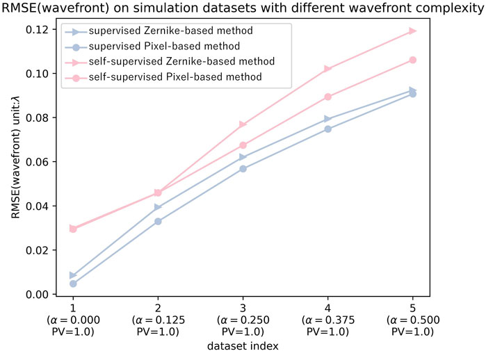
Figure 4. The average RMSE for each method on datasets with different wavefront complexity (datasets 1–5 in Table 1).

3.2 Effect of wavefront aberrations of different PVs on detection accuracy

Figure 5 shows the performance of the different methods for wavefront aberrations at different PVs for quantitative analysis. The last five datasets in Table 1 are selected for training and testing, respectively.

Figure 5

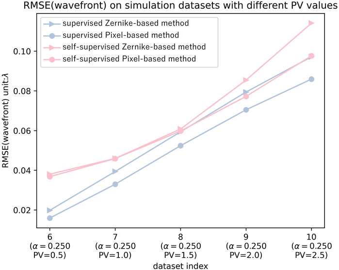
Figure 5. The average RMSE for each method on datasets with different wavefront PVs (datasets 6–10 in Table 1).

The following three conclusions can be drawn from Figure 5:

(1) Regardless of the training method employed, pixel-based approaches consistently outperform Zernike-based methods. Moreover, supervised training methods exhibit better performance across all PV ratios, accurately recovering low-frequency components within the wavefront. These findings align with those in section 3.1.

(2) The performance of self-supervised training methods is poor at PV = 0.5, but as PV increases, the accuracy of wavefront recovery gradually improves. This is because as the wavefront aberration decreases, the spot size of the PSF becomes smaller, containing less information, making it difficult for self-supervised methods to measure the difference between predicted wavefront and ground truth solely based on PSF.

(3) As PV increases, the gap between pixel-based and Zernike-based methods gradually widens (for both supervised and self-supervised methods), which differs from the conclusion in section 3.1. This demonstrates that Zernike-based methods are more challenged by higher PV wavefronts compared to more complex wavefronts.

3.3 Cross-dataset performance

Due to the challenge of obtaining a large number of labels in practical scenarios, supervised training inevitably faces the scenario of cross-dataset application, where the distribution of training and testing data differs. To simulate this situation. First, the supervised method is trained using the 1st dataset in Table 1 and tested with the 1st through 5th datasets, and the results are shown in Figure 6A. In addition, it is also trained using the 6th dataset in Table 1 and tested with the 6th through 10th datasets, and the results are shown in Figure 6B. Since self-supervised methods do not require wavefront labels during training, they can easily adapt the network to new distributions when dataset distributions change, avoiding this issue. Therefore, their results remain consistent and are the same as in Figures 4, 5.

Figure 6

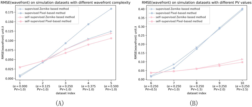
Figure 6. Cross-dataset test results. (A) Test results across datasets 1–5 in Table 1 (supervised network trained with dataset 1 only). (B) Test results for datasets 6–10 in Table 1 (supervised network trained with dataset 6 only).

The following two conclusions can be drawn from Figure 6:

(1) The larger the gap between the training and the test dataset, the worse the performance of the supervised methods. The supervised method is worse than the self-supervised method at both $a$ > 0.125 in Figure 6A and PV > 0.75 in Figure 6B. It proves that self-supervised methods are more suitable for use in real scenarios.

(2) An increase in PV leads to a more dramatic decrease in the performance of the supervised trained network compared to an increase in wavefront complexity. It is demonstrated that supervised networks are more sensitive to the aberration range.

In practice, real systems will be affected by more complicated effects, including the effects of air turbulence, high-order surface error of the mirrors, vibration, and the unknown distribution of noise, etc. In other words, it is usually difficult to obtain a large set of real labeled data that is used to train the network.

4 Experiment

In this work, an off-axis three-mirror anastigmatic (TMA) optical system is taken as the experimental optical system to verify the effectiveness of the proposed approach. The sketch and physical map of the experimental optical system are shown in Figures 7A, B, respectively. The interferometer (PhaseCam 4020) has two functions in this experiment. On one hand, it is used to measure wavefront maps which will serve as the reference value to evaluate the accuracy of different deep learning methods; on the other hand, the focus of the interferometer will serve as a point source and a PSF is finally obtained with CCD after the laser light (the wavelength is 632.8 nm) is reflected by the flat mirror. The aperture of the system is 500 mm, the focal length of the system is 6000 mm, and the CCD pixel size is 5.5 µm. It is important to note that the beam splitter introduces aberrations between the optical paths of the interferometer and the camera. These aberrations were calibrated and removed during the comparison to ensure precise results.

Figure 7

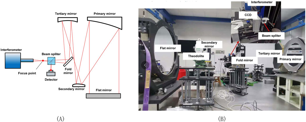
Figure 7. The sketch (A) and physical map (B) of the optical system used in the experiment.

In this experiment, 300 unlabeled PSF images acquired from real systems are collected to fine-tune the network trained on the simulated images. Besides, 20 labeled PSF images are collected for testing. To ensure diversity, we introduced different misalignments into the system before capturing each PSFs. In addition, we acquired data from five different fields of view (FoV), including the center FoV and four edge FoV. The size of each PSF image is 64 × 64.

The performance of different algorithms using the real dataset is summarized in Table 2. Because in practice, Zernike’s C5–C9 terms are of more interest than the higher-order terms, the performance of the model is measured here by the accuracy of the C5–C9 terms only. For supervised deep learning approaches, due to the challenge of acquiring a substantial amount of labeled real data, these methods typically train networks with simulated data and test them on real images. Considering the substantial discrepancies between simulated and real images (due to unknown high-frequency figure errors), these supervised approaches often struggle to achieve satisfactory results, with an average RMSE of about 0.110 $\lambda$ (here the RMSE is calculated using C5–C9). In contrast, self-supervised learning methods can fine-tune pre-trained networks with real images to adapt to real data distribution, thereby attaining superior performance. Importantly, the method proposed in this study retains high-frequency and low-frequency information in images, leading to higher detection accuracy than methods based on Zernike polynomials, reducing the average RMS to 0.020 $\lambda$ (λ = 632.8 nm).

Table 2

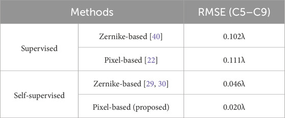
Table 2. Prediction accuracy of different deep learning methods on the real dataset.

A set of data is selected from the dataset for visualization, which has a major part of the aberration as astigmatism (C5 and C6), and the results are shown in Figure 8, where (A) includes the phase truth acquired by the interferometer and the PSF image acquired by the detector, (B) and (C) correspond to the Zernike-based and pixel-based methods with supervised training, respectively, and (D–E) are the corresponding methods with self-supervised training.

Figure 8

Figure 8. Comparison of wavefront prediction results for different detection methods on the real dataset. (A) shows the truth value of the phase map. (B–E) show the recovered wavefront maps using the supervised Zernike-based method, supervised pixel-based method, self-supervised Zernike-based method, and the proposed self-supervised pixel-based method, respectively. The RMSE between each predicted result and the true value, as well as the RMSE for the C5–C9 terms, are marked above the corresponding wavefront maps.

The following three conclusions can be drawn from Figure 8:

(1) By comparing the true phase with the phase recovered by the network, it can be seen that all methods recognize that the aberrations are dominated by astigmatism (C5) in this image. This demonstrates that the network can learn the relationship between PSF and aberration and maintains a certain level of recognition after changing the dataset regardless of which method is used.

(2) When the training methods are the same (both supervised or self-supervised training), the pixel-based approach outperforms the Zernike-based approach, proving that the former is more generalized and more suitable for applications in complex scenarios in real situations.

Table 3 shows some of the results of the interferometer measurements and network predictions. The values of astigmatism (C5/C6) and coma (C7/C8) correspond to the Fringe Zernike and they are both converted to Standard Zernike coefficients when calculating the RMS. The RMS for most of the results was around 0.018 $\lambda$ and the best and worst results are 0.009 $\lambda$ and 0.034 $\lambda$, respectively, as shown in the first and second rows of Table 3.

Table 3

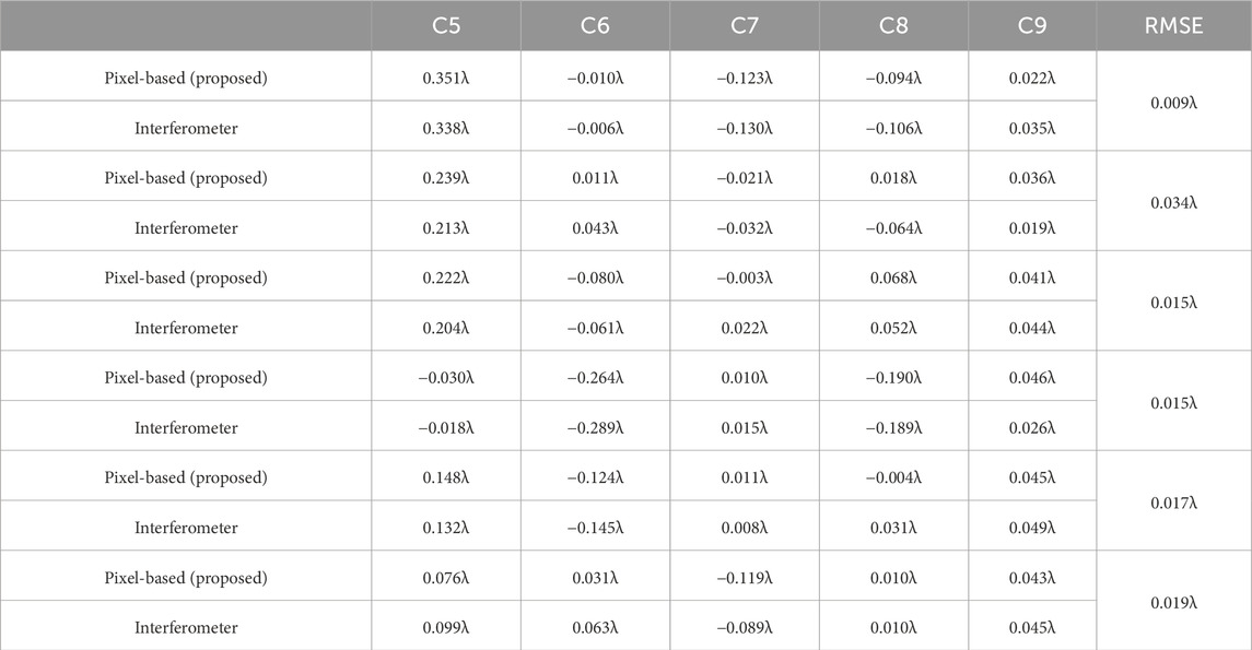
Table 3. Comparison of some network predictions with interferometer data (C5 to C9 coefficients for Fringe Zernike).

5 Ablation experiments

To further validate the effectiveness of the proposed method, ablation experiments were conducted using real datasets. The experimental results are summarized in Table 4, which compares the average RMSE of networks under different configurations. The low-frequency and high-frequency restrictive conditions correspond to Equations 5, 8, respectively. The training process followed the same approach as outlined in Section 4.

Table 4

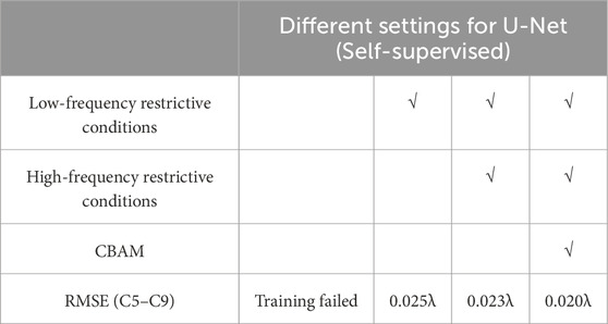
Table 4. Average RMSE for U-Net with different settings on real datasets (λ = 632.8 nm).

The results indicate that without any constraints, the pixel-based self-supervised method fails to produce accurate results. It leads to erroneous and discontinuous wavefronts. The addition of frequency constraints ensures the reliability of the network’s solution. Furthermore, the use of frequency-based restrictive conditions and the CBAM attention mechanism significantly enhances the detection accuracy. As these additional components are incrementally incorporated, the RMSE decreases from 0.025λ to 0.020λ (with a wavelength of λ = 632.8 nm), confirming the effectiveness of the proposed method.

6 Discussions

The effect of network size on wavefront sensing accuracy is investigated by applying three networks with different network sizes to a real dataset. These networks include the Atten-U-Net as introduced in Section 2.2, the Atten-U-Net-M with doubled network width, and the Atten-U-Net-L with both increased width and depth. The results are shown in Table 5 and Figure 9, where we can see that there is a gradual improvement in wavefront sensing accuracy with the increased complexity of the network architecture. This result demonstrates that deep learning methods can improve their accuracy to some extent by scaling up computational efforts.

Table 5

Table 5. Average RMSE for networks with different sizes on real datasets (λ = 632.8 nm).

Figure 9

Figure 9. Box plots of RMSE between the recovered wavefront and the true wavefront for networks with different sizes on real datasets. It can be seen that after increasing the network size, the accuracy is improved gradually.

7 Conclusion

In this paper, we propose a self-supervised deep learning method based on pixel dimensionality, which enhances the accuracy of detection by constraining the output of the network through low-pass filtering and high-pass filtering to ensure that some of the high-frequency information is retained under the premise of phase continuity.

We first confirm the accuracy of the supervised learning method is higher than the self-supervised learning method on a simulation dataset because a large amount of labeled data provides a clear learning target for the network. However, when transferred to a real scenario lacking a large number of labels, the network trained on the simulated data performs poorly in terms of detection accuracy due to the discrepancy between simulation and reality. In contrast, self-supervised learning methods can directly utilize real data for fine-tuning and adapting to the real data distribution, thus achieving satisfactory results.

In addition, experiments on both simulated and real datasets show that when dealing with complex wavefronts, the pixel-based prediction strategy proposed in this paper can effectively retain more high-frequency information and achieve higher detection accuracy compared to the Zernike polynomial-based approach.

We also explore methods to further improve detection accuracy, including the increase of network width and depth. The experimental results show that all these methods can effectively improve the detection accuracy. By increasing the complexity of the network, we can improve the detection accuracy without relying on additional prior knowledge.

Data availability statement

The raw data supporting the conclusions of this article will be made available by the authors, without undue reservation.

Author contributions

YL: Conceptualization, Data curation, Formal Analysis, Funding acquisition, Investigation, Methodology, Project administration, Resources, Software, Supervision, Validation, Visualization, Writing–original draft, Writing–review and editing. XB: Formal Analysis, Software, Writing–review and editing. BX: Writing–review and editing. CZ: Writing–review and editing. YG: Writing–review and editing. SX: Writing–review and editing. GJ: Conceptualization, Data curation, Investigation, Methodology, Writing–original draft, Writing–review and editing.

Funding

The author(s) declare that financial support was received for the research, authorship, and/or publication of this article. This study was supported by the National Natural Science Foundation of China (61905241).

Conflict of interest

The authors declare that the research was conducted in the absence of any commercial or financial relationships that could be construed as a potential conflict of interest.

Generative AI statement

The authors declare that no Generative AI was used in the creation of this manuscript.

Publisher’s note

All claims expressed in this article are solely those of the authors and do not necessarily represent those of their affiliated organizations, or those of the publisher, the editors and the reviewers. Any product that may be evaluated in this article, or claim that may be made by its manufacturer, is not guaranteed or endorsed by the publisher.

References

1. Gonsalves RA. Phase retrieval and diversity in adaptive optics. Opt Eng (1982) 21:829–32. doi:10.1117/12.7972989

CrossRef Full Text | Google Scholar

2. Tehrani KF, Zhang Y, Shen P, Kner P. Adaptive optics stochastic optical reconstruction microscopy (AO-STORM) by particle swarm optimization. Biomed Opt Express (2017) 8(11):5087–97. doi:10.1364/BOE.8.005087

PubMed Abstract | CrossRef Full Text | Google Scholar

3. Wang D, Yuan Q, Yang Y, Zhang X, Chen L, Zheng Y, et al. Simulational and experimental investigation on the wavefront sensing method based on near-field profile acquisition in high power lasers. Opt Commun (2020) 471:125855. doi:10.1016/j.optcom.2020.125855

CrossRef Full Text | Google Scholar

4. Xu H, Wu J. Sparse scanning hartmann wavefront sensor. Opt Commun (2023) 530:129148. doi:10.1016/j.optcom.2022.129148

CrossRef Full Text | Google Scholar

5. Guan H, Zhao W, Wang S, Yang K, Zhao M, Liu S, et al. Higher-resolution wavefront sensing based on sub-wavefront information extraction. Front Phys (2024) 11, 1336651. doi:10.3389/fphy.2023.1336651

CrossRef Full Text | Google Scholar

6. Schwertner M, Booth M, Wilson T. Wavefront sensing based on rotated lateral shearing interferometry. Opt Commun (2008) 281:210–6. doi:10.1016/j.optcom.2007.09.025

CrossRef Full Text | Google Scholar

7. Ju G, Qi X, Ma H, Yan C. Feature-based phase retrieval wavefront sensing approach using machine learning. Opt Express (2018) 26:31767–83. doi:10.1364/OE.26.031767

PubMed Abstract | CrossRef Full Text | Google Scholar

8. Booth MJ. Wavefront sensorless adaptive optics for large aberrations. Opt Lett (2007) 32(1):5–7. doi:10.1364/ol.32.000005

PubMed Abstract | CrossRef Full Text | Google Scholar

9. Linhai H, Rao C. Wavefront sensorless adaptive optics: a general model-based approach. Opt Express (2011) 19(1):371–9. doi:10.1364/oe.19.000371

PubMed Abstract | CrossRef Full Text | Google Scholar

10. Booth MJ. Wave front sensor-less adaptive optics: a model-based approach using sphere packings. Opt Express (2006) 14(4):1339–52. doi:10.1364/oe.14.001339

PubMed Abstract | CrossRef Full Text | Google Scholar

11. Yue D, Nie H. Wavefront sensorless adaptive optics system for extended objects based on linear phase diversity technique. Opt Commun (2020) 475:126209. doi:10.1016/j.optcom.2020.126209

CrossRef Full Text | Google Scholar

12. Goel N, Dinesh GS. Wavefront sensing: techniques, applications, and challenges. Atmos Ocean Opt (2024) 37:103–17. doi:10.1134/S1024856023700148

CrossRef Full Text | Google Scholar

13. Kong F, Cegarra Polo M, Lambert A. Fpga implementation of shack–Hartmann wavefront sensing using stream-based center of gravity method for centroid estimation. Electronics (2023) 12:1714. doi:10.3390/electronics12071714

CrossRef Full Text | Google Scholar

14. Wang K, Song L, Wang C, Ren Z, Zhao G, Dou J, et al. On the use of deep learning for phase recovery. Light Sci Appl (2024) 13:4. doi:10.1038/s41377-023-01340-x

PubMed Abstract | CrossRef Full Text | Google Scholar

15. Goi E, Schoenhardt S, Gu M. Direct retrieval of zernike-based pupil functions using integrated diffractive deep neural networks. Nat Commun (2022) 13:7531. doi:10.1038/s41467-022-35349-4

PubMed Abstract | CrossRef Full Text | Google Scholar

16. Chen H, Zhang H, He Y, Wei L, Yang J, Li X, et al. Direct wavefront sensing with a plenoptic sensor based on deep learning. Opt Express (2023) 31:10320–32. doi:10.1364/oe.481433

PubMed Abstract | CrossRef Full Text | Google Scholar

17. Guzmán F, Tapia J, Weinberger C, Hernández N, Bacca J, Neichel B, et al. Deep optics preconditioner for modulation-free pyramid wavefront sensing. Photon Res (2024) 12:301–12. doi:10.1364/prj.502245

CrossRef Full Text | Google Scholar

18. Xin Q, Ju G, Zhang C, Xu S. Object-independent image-based wavefront sensing approach using phase diversity images and deep learning. Opt Express (2019) 27:26102–19. doi:10.1364/oe.27.026102

PubMed Abstract | CrossRef Full Text | Google Scholar

19. Zhou Z, Zhang J, Fu Q, Nie Y. Phase-diversity wavefront sensing enhanced by a fourier-based neural network. Opt Express (2022) 30:34396–410. doi:10.1364/oe.466292

PubMed Abstract | CrossRef Full Text | Google Scholar

20. Zhou Z, Fu Q, Zhang J, Nie Y. Generalization of learned fourier-based phase-diversity wavefront sensing. Opt Express (2023) 31:11729–44. doi:10.1364/oe.484057

PubMed Abstract | CrossRef Full Text | Google Scholar

21. Ge X, Zhu L, Gao Z, Wang N, Zhao W, Ye H, et al. Target-independent dynamic wavefront sensing method based on distorted grating and deep learning. Chin Opt Lett (2023) 21:060101. doi:10.3788/col202321.060101

CrossRef Full Text | Google Scholar

22. Siddik AB, Sandoval S, Voelz D, Boucheron LE, Varela L. Deep learning estimation of modified zernike coefficients and recovery of point spread functions in turbulence. Opt Express (2023) 31:22903–13. doi:10.1364/OE.493229

PubMed Abstract | CrossRef Full Text | Google Scholar

23. Wang K, Zhang M, Tang J, Wang L, Hu L, Wu X, et al. Deep learning wavefront sensing and aberration correction in atmospheric turbulence. PhotoniX (2021) 2:8–11. doi:10.1186/s43074-021-00030-4

CrossRef Full Text | Google Scholar

24. Zhuang Y, Wang D, Deng X, Lin S, Zheng Y, Guo L, et al. High robustness single-shot wavefront sensing method using a near-field profile image and fully-connected retrieval neural network for a high power laser facility. Opt Express (2023) 31:26990–7005. doi:10.1364/oe.496020

PubMed Abstract | CrossRef Full Text | Google Scholar

25. Hu S, Hu L, Gong W, Li Z, Si K. Deep learning based wavefront sensor for complex wavefront detection in adaptive optical microscopes. Front Inf Technol Electron Eng (2021) 22:1277–88. doi:10.1631/fitee.2000422

CrossRef Full Text | Google Scholar

26. Agarwal H, Mishra D, Kumar A. A deep-learning approach for turbulence correction in free space optical communication with laguerre–Gaussian modes. Opt Commun (2024) 556:130249. doi:10.1016/j.optcom.2023.130249

CrossRef Full Text | Google Scholar

27. Smith J, Cranney J, Gretton C, Gratadour D. Image-to-image translation for wavefront and point spread function estimation. J Astron Telesc Instruments, Syst (2023) 9, 019001. doi:10.1117/1.jatis.9.1.019001

CrossRef Full Text | Google Scholar

28. Zhao J, Wang C, Yang X. Wavefront reconstruction method based on improved u-net. In: 2023 6th international conference on computer network, electronic and automation (ICCNEA) (2023). p. 262–6. doi:10.1109/ICCNEA60107.2023.00063

CrossRef Full Text | Google Scholar

29. Ning Y, He Y, Li J, Sun Q, Xi F, Su A, et al. Unsupervised learning-based wavefront sensing method for Hartmanns with insufficient sub-apertures. Opt Continuum (2024) 3:122–34. doi:10.1364/optcon.506047

CrossRef Full Text | Google Scholar

30. Xu Y, Guo H, Wang Z, He D, Tan Y, Huang Y. Self-supervised deep learning for improved image-based wave-front sensing. Photonics (2022) 9:165. doi:10.3390/photonics9030165

CrossRef Full Text | Google Scholar

31. Ge X, Zhu L, Gao Z, Wang N, Ye H, Wang S, et al. Object-independent wavefront sensing method based on an unsupervised learning model for overcoming aberrations in optical systems. Opt Lett (2023) 48:4476–9. doi:10.1364/OL.499340

PubMed Abstract | CrossRef Full Text | Google Scholar

32. Rigaut FJ, Véran J-P, Lai O. Analytical model for shack-hartmann-based adaptive optics systems. Adaptive Opt Syst Tech (1998) 3353:1038–48. doi:10.1117/12.321649

CrossRef Full Text | Google Scholar

33. Ronneberger O, Fischer P, Brox T. U-net: convolutional networks for biomedical image segmentation. In: Proceedings medical image computing and computer-assisted intervention–MICCAI 2015: 18th international conference Munich, Germany, October 5–9, 2015 (2015) 234–41. doi:10.1007/978-3-319-24574-4_28

CrossRef Full Text | Google Scholar

34. Woo S, Park J, Lee J-Y, Kweon IS. Cbam: convolutional block attention module. In: Proceedings of the European conference on computer vision (ECCV) (2018). p. 3–19. doi:10.48550/arXiv.1807.06521

CrossRef Full Text | Google Scholar

35. Johnson JF. Modeling imager deterministic and statistical modulation transfer functions. Appl Optics (1993) 32:6503–13. doi:10.1364/ao.32.006503

PubMed Abstract | CrossRef Full Text | Google Scholar

36. Lightsey PA, Knight JS, Bolcar MR, Eisenhower MJ, Feinberg LD, Hayden WL, et al. Optical budgeting for luvoir. In: Space telescopes and instrumentation 2018: optical, infrared, and millimeter wave (2018) 10698. doi:10.1117/12.2312256

CrossRef Full Text | Google Scholar

37. Girshick R. Fast r-cnn. In: Proceedings of the IEEE international conference on computer vision Santiago, Chile, 07-13 December 2015, (IEEE) (2015). p. 1440–8. doi:10.1109/TPAMI.2016.2577031

CrossRef Full Text | Google Scholar

38. Wang Z, Bovik AC, Sheikh HR, Simoncelli EP. Image quality assessment: from error visibility to structural similarity. IEEE Trans image Process (2004) 13:600–12. doi:10.1109/TIP.2003.819861

PubMed Abstract | CrossRef Full Text | Google Scholar

39. Andrews LC. An analytical model for the refractive index power spectrum and its application to optical scintillations in the atmosphere. J Modern Optics (1992) 39:1849–53. doi:10.1080/09500349214551931

CrossRef Full Text | Google Scholar

40. Andersen T, Owner-Petersen M, Enmark A. Neural networks for image-based wavefront sensing for astronomy. Opt Lett (2019) 44:4618–21. doi:10.1364/ol.44.004618

PubMed Abstract | CrossRef Full Text | Google Scholar

41. Orban de Xivry G, Quesnel M, Vanberg P-O, Absil O, Louppe G. Focal plane wavefront sensing using machine learning: performance of convolutional neural networks compared to fundamental limits. Mon Notices R Astron. Soc. (2021) 505:5702–13. doi:10.1093/mnras/stab1634

CrossRef Full Text | Google Scholar