Multiscale Granger dependencies in the precipitation network of the island of Sicily

The island of Sicily has been displaying unusual rainfall behavior and unexpected extreme precipitation events in recent decades. In this study, we investigate the Granger causal (GC) dependencies in the network of precipitation measurement sites of Sicily at different timescales (every 10 min, 1 h, 6 h, 12 h, and 24 h). We study, across seasons and years, different parameters that characterize the GC dependencies: the total in/out-degree of nodes, the total in/out strength of nodes, the total number of links in the network, the number of eastward/westward links, the strength of eastward/westward links, and the maximum strength of links. We then investigate GC statistic intensities, focusing on the temporal evolution of maximum values over multiple timescales. Our study of precipitation patterns in Sicily indicates that, since 2013, the southern regions near Mount Etna (Catania, Siracusa, and Ragusa) have been increasingly affected, while the western areas (Trapani, Palermo, and Agrigento) have been the most affected. Granger causality networks reveal scale-invariant dependencies, with stronger and sparser connections at timescales that extend beyond 6 h, with a notable westward flow of predictive information. These patterns, which are consistent across seasons, suggest localized perturbation fronts, with stronger links indicating a more significant influence on westward predictions. This study highlights shifts in Sicily’s water cycle that call for adaptive management strategies in the face of the increasing frequency of extreme events.

1 Introduction

1.1 Overview

Climate changes at the global scale manifest themselves through a slight and constant increase in parameters such as sea surface temperature, usually followed by the onset of extreme weather events like heatwaves, droughts, wildfires, tropical cyclones, and extreme precipitation. The literature reports that extreme weather events are becoming more frequent and intense [1] and that this entails increased risks that can seriously affect social and economic stability along with physical and mental health [2]. Therefore, the characterization of climatic variables and the detection of their temporal trends enhance both our awareness of what is happening and our ability to better forecast what is likely to occur. Rainfall constitutes an important climatic variable, as lack of it can lead to severe droughts, and its excess can trigger catastrophic events. Extreme precipitation is one of the most dangerous and extreme weather events since its occurrence is hard to predict, and consequently, it is difficult to warn populations and provide emergency assistance [3]. The Sixth Assessment Report (AR6) of the Intergovernmental Panel on Climate Change (IPCC) [4] pointed out that, since the 1950s, the frequency and intensity of heavy precipitation events has been growing globally. Disasters generated by heavy precipitation represent only the immediate consequence of an extreme phenomenon: long-lasting effects that disrupt the equilibrium of local ecosystems and biospheres along with human structures and activities. The increasing extremity of precipitation volumes and the upward trend of extreme precipitation events are signals of a deeper change in the dynamics of rainfall regimes.

The Mediterranean basin is a region at the boundary of larger climatic systems: it is characterized by high spatial and temporal variability and is one of the regions most affected by climate change and its effects [5]. The onset and recurrence of such events is an indicator of the increasingly extreme Mediterranean pluviometric regime and is correlated with the fluctuations in the NAO (North Atlantic Oscillation), which influences the location of permanent cyclones and anticyclones around the basin [6]. Observations in the Mediterranean region until the 2000s showed a general precipitation decrease over both the eastern and western Mediterranean basins during the winter months [7]. In addition, extreme rainfall events are becoming more frequent in winter in the eastern Mediterranean part of the basin and in autumn in the western part [8]. Because of its particularly central position with respect to the Mediterranean basin, Sicily has recently experienced violent flash floods and more severe dry periods. The majority of observed extreme rainfall events are concentrated in summer and mid-autumn [9–11], and their occurrence has become more frequent and intense, particularly in the eastern part of the island. In contrast, winter precipitation volumes are decreasing [12, 13].

1.2 Granger causality and climate systems

Gaining knowledge of and measuring rainfall variations above Sicily is a crucial challenge for both researchers and authorities. Anomalous events such as flash floods or prolonged droughts are hard to predict and lead to consequences well-known in other parts of the world: lack of water for plants and animals, including humans, and disruption of urban infrastructure, economic activity, and civic life. Prolonged dry periods followed by prolonged wet periods also have a deep impact on soil settlement and water reservoirs, influencing the viability and biodiversity of vegetation. It is thus important to investigate rainfall behaviors and their dependencies, such as appropriate spatial and temporal resolution. Many authors have investigated the spatial and temporal correlation between climatic variables by performing the Granger causality test,—a linear statistical method to quantify the gain in pairwise predictability of time series [14, 33]. This approach has been successfully employed to unravel connections between climatic parameters such as the drought index [15] or sea surface temperature [16] and oscillations in the atmospheric general circulation such as ENSO (El Niño Southern Oscillation) to model and forecast climatic variables such as extreme precipitation [17] and to explore correlations between pollutants and temperature [18]. Granger causality networks have been employed in order to constrain precipitation projections under climate change [19] or to capture complex rainfall patterns with higher resolution in the memory of the system [20]. In particular, the scale-invariant nature of precipitation events has been demonstrated to be a characteristic of complex precipitation processes [21]; the application of Tsallis q-statistics [22] in this context has been a valuable tool for capturing the out-of-equilibrium nature of precipitation data in addition to the presence of long-range correlations and memory effects.

1.3 Multiscale analysis and rainfall dynamics

Scaling-type regularities in data provide valuable insights into the underlying mechanisms of data generation. These regularities, often observed as patterns that remain consistent or follow predictable relationships across different scales, serve as “stylized facts” that any theoretical model should aim to replicate [23]. For example, scaling laws are evident when variables in a system follow a power-law distribution, as is the case with precipitation [10]. Such distributions reveal that the relationships between variables remain consistent regardless of the timescale of observation. In practical terms, these regularities suggest that the same underlying rules or dynamics apply whether one looks at small or large scales of a system, and often provide insights into the fundamental processes that drive complex systems. This makes them valuable for modeling because they act as a benchmark—any theoretical model that aims to describe the system should ideally be able to reproduce these scaling patterns. In the context of precipitation studies, temporal scaling behavior has been investigated in many areas, such as the forecasting of hydrological processes through machine learning classification methods [24], the implementation of the computation of rainfall-erosion soil indicators [25], rainfall run-off [26], the reduction of uncertainty propagation [27], and the analysis spatio-temporal web sensors [28]. Another intriguing element in the implementation of hydrological calculations deals with multifractal theory [29], since the scaling properties of temporal precipitation dynamics display multidimensional fractal behavior, indicating that the rainfall process can be described by a multiplicative cascading process [30]. Recent advancements in transfer entropy, which is equivalent to Granger causality for Gaussian variables, have demonstrated its utility in handling climatic variables. For instance, Smith et al. [31] explored these concepts in depth, offering valuable insights into their application to climate-related research. In light of the work conducted using the above methods, we investigate here for the first time the Granger dependencies in the precipitation network of the island of Sicily, taking into account only one parameter (precipitation records) and exploring its spatial configuration at different temporal resolutions (10 min, 1 h, 6 h, 12 h, and 24 h) over 22 years. First, we built our network by using precipitation records from nine rain gauges over one year as nodes and the Granger causality (GC) strength between their seasonal time series as links for the years 2002–2023. We have studied, across seasons and years, different parameters: the total in/out-degree of nodes, the total in/out strength of nodes, the total number of links in the network, the number of eastward/westward links, the strength of eastward/westward links, and the maximum strength of links across seasons and years.

2 Data and methods

2.1 Dataset

The dataset, available on request from SIAS (Sicilian Agrometeorological Informative System—www.sias.regione.sicilia.it), contains the hourly precipitation records of nine rain gauges on the island of Sicily from 2002 to 2023 (Figure 1). These rain gauges from Messina (ME), Siracusa (SR), Catania (CT), Ragusa (RG), Enna (EN), Caltanissetta (CL), Agrigento (AG), Palermo (PA), and Trapani (TP) are only subsets of the robust and extensive rain gauge network comprising 96 pluviometric stations.

Figure 1

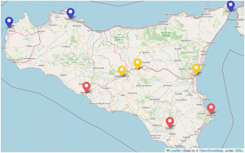
Figure 1. Selected subset of the SIAS network represented by nine rain gauges located in the main cities of Sicily, Italy.

2.2 Granger causality

In the context of linear regression [32–34], any target series Y can be considered the weighted sum of its past states plus an error term. Then, it is possible to make a second model by also summing the past states of a source variable. The former, Equation 1, is referred to as a “reduced model”, and the latter, Equation 2, as a “full model”.

$Y_t={\displaystyle \sum _{m=1}^p}{a}_m{Y}_{t-m}+{ϵ}_t(1)$

$Y_t={\displaystyle \sum _{m=1}^p}{a}_m{Y}_{t-m}+{\displaystyle \sum _{m=1}^q}{b}_m{X}_{t-m}+{ϵ}_t(2)$

Equation 1 represents a univariate autoregressive process in which $Y_t$ depends solely on its own past values up to $p$ lags. The coefficients $a_m$ measure the influence of the past values. Equation 2 extends the autoregressive model by including the past values of another time series, $X_t$ (up to $q$ lags). The coefficients $b_m$ capture the influence of $X_t$ on $Y_t$. If the coefficients $b_m$ are statistically significant, this suggests that $X_t$ Granger causes $Y_t$. In both equations, ${ϵ}_t$ accounts for the unexplained variability. Since in this study X and Y are two different rain gauge time series, in the full model, the future states of the target rain gauge Y are predicted by its own past states p and the previous states of the source X. In the reduced model, only the target is taken into account. The GC strength, defined as the logarithmic ratio between the variance of the error term of the reduced model and that of the full model, quantifies the soundness of the regressions and tests whether the full model improves the predictability of the target time series. Therefore, the existence of a link means that the past source contains information about the future of the target. The stronger the connection, the higher the predictability of the target; in other words, the influence of the source on the future of the target.

2.3 Granger causality networks

Following a procedure introduced in [35] in the context of financial markets, we performed the Granger causality test between couples of nodes—a source node and a target node, where each node represents the hourly precipitation time series of a rain gauge in a given year during a season. The whole dataset consists of 22 years of hourly precipitation records: we decided to extract subsets with a length of 3 months (i.e., one season). Following the choice usually employed in econometrics, we operated on log-returs of $P_t$ Equation 3, with the aim of achieving stable series [35]:

$r_t=\ln \left(\frac{P_t}{P_{t-1}}\right)=\ln \left(P_t\right)-\ln \left(P_{t-1}\right)(3)$

where $r_t$ is the log return at time $t$, $P_t$ is the precipitation record at time $t$, and $P_{t-1}$ is the precipitation record at time $t-1$.

In order to obtain consistent results, the main assumption for Granger causality is that the residuals in (1) and (2) must follow a Gaussian distribution. Therefore, we performed the Jarque–Bera test [36], a statistical goodness-of-fit test that assesses whether the skewness and kurtosis of the sample data align with those expected from a normal distribution by computing ${\sigma }_{JB}$ Equation 4, as follows:

${\sigma }_{JB}=\frac{n}{6}\left(S^2+\frac{{\left(K-3\right)}^2}{4}\right)(4)$

where $n$ is the sample size, $S$ represents its skewness, and $K$ represents its kurtosis. Such a test calculates nonnegative statistics, where values of ${\sigma }_{JB}$ significantly greater than 0 indicate a deviation from normality in the data. We carried out the Jarque–Bera test on the log-return time series, obtaining values near to 0 for all seasons and years. Since the Granger stability assumption is fulfilled for each quarterly time series, we generated 22 weighted and directed networks (one per year) for each season (Figure 2). The grangercausalitytests function in Python’s statsmodels library utilizes the GC statistics to evaluate Granger causality. This function conducts a series of hypothesis tests to determine whether the inclusion of lagged values from one-time series significantly enhances the predictability of another, indicating a potential causal relationship. Among the outputs provided, the $SS{R}_{\mathit{ftest}}$ (sum of squared residuals GC test) result includes the GC statistics and its associated p-value. This test compares the variance explained by the lagged predictor series to the variance left unexplained, thereby quantifying the predictive power added by the lagged terms. We set the p-value threshold at 0.01 and a lag of one row with respect to each timescale (e.g., 10 min for 10 min resolution, 1 h for hourly resolution, and so on). We explored the networks by separately analyzing the behavior of nodes and links generating appropriate grids that enable a synoptic vision of the parameters studied—the total in/out-degree of nodes, the total in/out strength of nodes, the total number of links in the network, the number of eastward/westward links, the strength of eastward/westward links, and the maximum link strength across seasons and years.

Figure 2

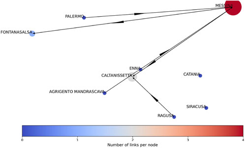
Figure 2. Example of a 24 h timescale Granger network for the winter of 2002. The color of the nodes (from blue to red) is proportional to their total degree (the total number of node links), and their size shows the strength of the GC statistics (the sum of the strengths of the node’s links). The position of the nodes in the graph approximately corresponds to the geographical positions of the sites. Directed edges are reported as thin black arrows.

2.4 Steps of the method

Our method is based on the following steps:

1. Computation of logarithmic returns

2. Application of Granger causality on quarterly time series by means of the function grangercausalitytests from Statsmodel’s Python package: the test was performed between each couple of nodes.

3. Building of the Granger network.

4. Seasonal grouping of the networks across years

5. Analysis of total in/out-degree and strength of nodes

6. Analysis of the total number of links in the network

7. Analysis of the total number and strength of eastward/westward links in the network

8. Analysis of the maximum link strength across seasons and years

3 Results

We started by focusing on the nodes, considering separately the in- and out-link networks over the years through a synoptic seasonal network grid. In Figure 3, there is an example of this view for the winter season: the nodes corresponding to the nine rain gauges, ordered from west (TP, Trapani, bottom) to east (ME, Messina, top), are reported in the $y$-axis as a function of the years ($x$-axis), so that each vertical line represents a single network in a given year. In particular, we reported an example of winter out-link networks at 12 h time resolution. The color of the nodes (from blue to red) indicates the out-degree (i.e., the total number of out-links of the node), while their size is proportional to the strength of the GC statistics (i.e., the sum of the strength of the out-links of the node). Colors are normalized to the max out degree across years and sizes to the max strength across years. In Figure 4, we also plotted for the 2002 winter season at the 1 h timescale the total sum of the in-link strength of the GC statistics for each node—for each rain gauge. The Trapani, Palermo, and Messina stations, located on the Tyrrhenian coast, are colored in blue. Yellow is the color for Catania, Enna, and Caltanissetta, located in the central area near Mount Etna. The red stations are Ragusa, Siracusa, and Agrigento on the southern coast.

Figure 3

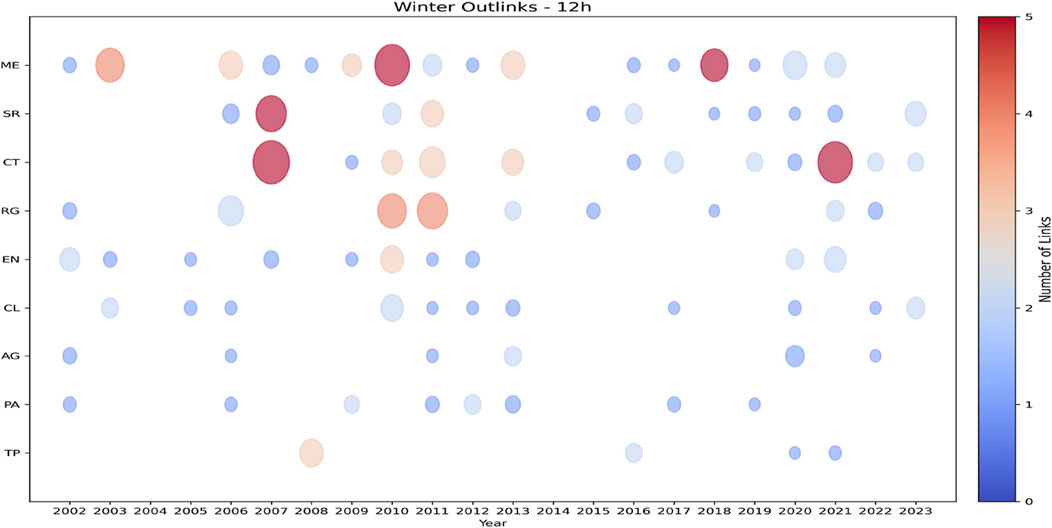
Figure 3. 2D grid of winter out-link networks at the 12 h timescale. Years are placed on the x-axis, and the nine rain gauges ordered east (ME) to west (TP) are plotted on the y-axis, so that each vertical line represents a single network in a single year. The color of the nodes (from blue to red) is proportional to their out-degree (i.e., the total number of out-links), and their size shows the strength of the GC statistics (i.e., the sum of the strengths of the out-links).

Figure 4

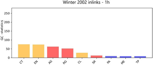
Figure 4. Example of the total sum of in-link strengths of the GC statistics per node for winter 2002 at the 1 h timescale, reported on the $y-axis$. Nodes on the $x-axis$ are arranged in ascending order. Blue stands for Trapani, Palermo, and Messina stations, which are located on Tyrrhenian coast. Yellow is the color of Catania, Enna, and Caltanissetta, in the central area near Mount Etna. Red is for the stations of Ragusa, Siracusa, and Agrigento, on the southern coast.

By integrating the results shown in the previous two figures, we were able to highlight the network dynamics in their spatial resolution. It appears that Messina is the city less involved in the dynamics of the Granger networks across all seasons and timescales. Palermo and Trapani, also on the Tyrrhenian coast, are the most influenced areas since the 6 h timescale. The central nodes of Catania, Enna, and Caltanissetta play, as expected, a role both as influencing and influenced areas; in particular, the Catania results are strongly connected to other nodes, especially after 2012. Siracusa and Ragusa, located on the southern coast, are often involved as influencing regions, while Agrigento is usually an area strongly influenced by other nodes. From a seasonal point of view, the most relevant shape is observed in summer, when the area most influenced is Palermo to 2012 across all timescales, and also in autumn, when the same situation arises for Agrigento. Moreover, the highest number of out-links and out-strength per node comes after 2012 in summer and autumn. Up to the 12 h timescale, the nodes with a high in/out degree do not coincide with those with high in/out strength (i.e., the red nodes on the grid are not the largest). At the level of the 24 h timescale, it is possible to observe that the two characteristics always belong to the same node, which appears to be a peculiarity of this temporal scale across all seasons.

Focusing on the GC network links, the total number of possible links in any network is given by $n_{(tot)}=n(n-1)$. In this study, each network consists of $n=9$ nodes, and so the total number of possible links is $n_{(tot)}=72$. In the two-dimensional plot reported in Figure 5, we addressed the seasonal behavior of the global number of links present in each Granger network across years for the 24 h timescale. By inspecting the global number of links across years, seasons, and timescales, the summer season at the 10-min scale appears to be the network with the highest number of $n_{(tot)}$, as it reaches the value of 50 connections. For the other seasons and time-scales, $n_{(tot)}$ varies from 20 to 30, except for winter and spring at the 24 h resolution, since $n_{(tot)}\le 10$. For winter and spring, $n_{(tot)}$ increases or at least remains constant after 2012 across all timescales. The same is true for summer but after 2007. The behavior of autumn is more peculiar, as, since 2012, the total number of connections starts to oscillate yearly.

Figure 5

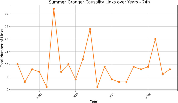
Figure 5. Seasonal global number of links across years for the summer season at the 24-h timescale: $y$-axis represents the total number of links present in each Granger network as a function of years ($x$-axis).

Going deeper into the network’s temporal dynamics, we chose the westward and eastward directions of the Granger networks in order to determine whether a privileged path exists across seasons and years. We analyzed this issue by plotting the seasonal number of eastward (blue) and westward (red) links over multiple years for each timescale. For example , in Figure 6 we reported the spring season for the 24h timescale. We found also that at the 10 min timescale, the number of westward links is comparable to the number of eastward links. Westward connections emerged as the privileged direction for all seasons at 1 h, 6 h, and 12 h, while for summer this was also the case for the 24 h timescale. At the latter timescale, in winter, westward becomes the preferred direction for consecutive years after 2012. For spring, this trend is evident before 2012, while for autumn the pattern oscillates across all 22 years.

Figure 6

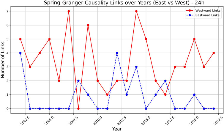
Figure 6. Spring global number of eastward (blue) and westward (red) links over multiple years at the 24-h timescale.

Finally, as displayed in Figure 7, we investigated the magnitude of the GC-statistical connections by generating $2\times 22$ matrices per season for each timescale, where the two rows represent the sum of the weight of eastward and westward links across the networks. The columns refer to individual years. The cool–warm color map is normalized across years and directions for each season and timescale. The results show that the higher values are westward across all seasons and timescales and are usually observed after 2012. Summer displays the highest values of the GC statistics across all seasons and timescales, whereas, for other seasons, the link strengths are comparable. In Figure 8 we also reported the behavior of the maximum GC statistic intensity computed across all seasons and over each timescale. Circular markers refer to the 2002–2012 interval, and triangular markers refer to the 2013–2023 period. Fully filled markers represent eastward records and unfilled markers indicate westward records. The results confirm the behavior observed in the previous figure and highlight that the highest maxima were observed after 2012. Moreover, the strength of the GC statistics during winter, spring, and autumn decreases from 1 h up to 24 h resolution. Around summer, the trend appeared to be more pronounced as the decline is drastic and stops at the 12 h timescale.

Figure 7

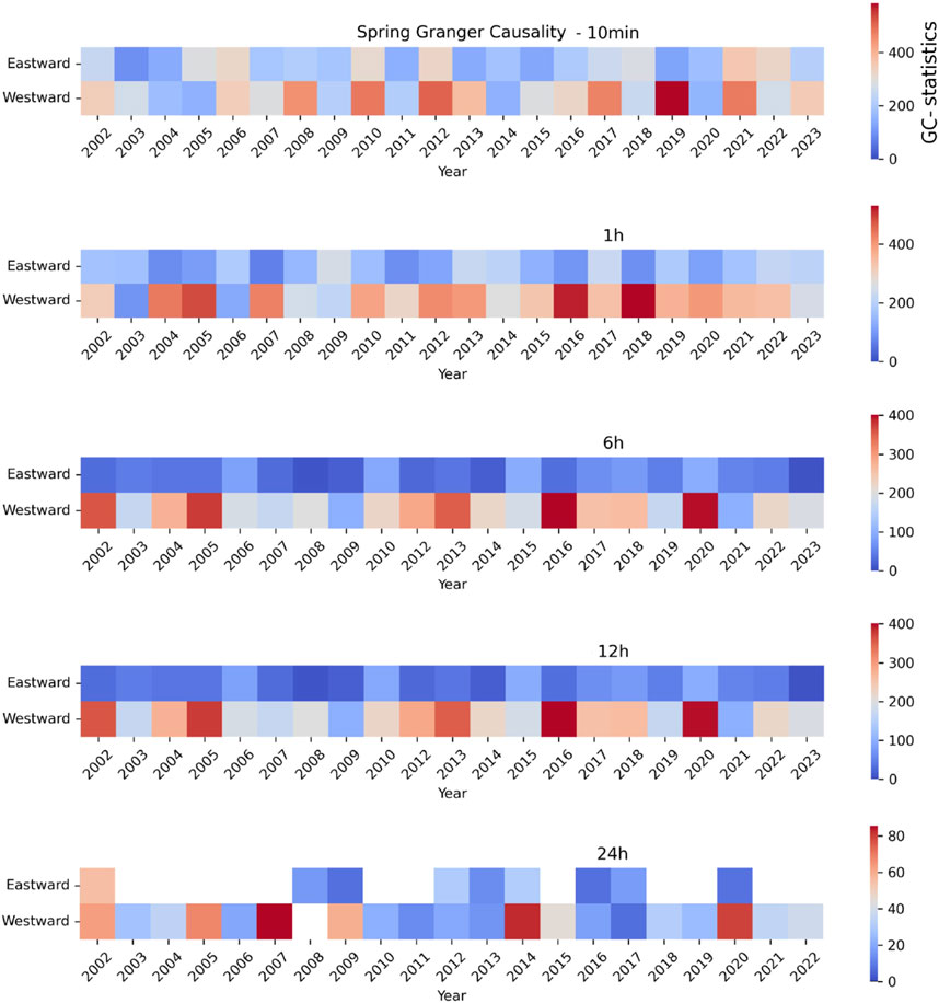
Figure 7. Matrices $2x22$ per season for each timescale. The two rows represent the sum of the weight of eastward and westward links across the networks. The columns refer to individual years. The cool–warm color map is normalized across years and directions for each season and timescale. From top to bottom: 10 min, 1 h, 6 h, 12 h, and 24 h.

Figure 8

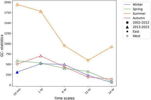
Figure 8. Behavior of the maximum GC statistic intensity computed across all seasons and timescales: on the $y$-axis is reported the intensity of the GC statistics, on the $x$-axis are shown multiple timescales. Blue, green, yellow, and red stand respectively for winter, spring, summer, and autumn. Circular markers refer to the 2002–2012 interval; triangular markers are related to the 2013–2023 period. Filled markers represent eastward records; unfilled markers indicate westward ones.

4 Discussion and conclusion

These results reveal that, across Sicily, the southern areas near Mount Etna—Catania, Siracusa, and Ragusa—have become the most affected since 2013, while Trapani, Palermo, and Agrigento are the most affected. Messina’s limited presence in the Granger network may reflect its unique coastal location at the convergence of the Nebrodi, Peloritani, and Etna regions, hinting at distinctive local dynamics. This configuration holds across all timescales and seasons, revealing a spatial scale invariance within the temporal one. Over 2002–2012, the higher number of connections across all seasons up to the 6 h timescale indicates a homogeneous dependence over the whole island, reflecting a high reciprocal predictability. From the 12 h timescale, many connections start to disappear and result in a sparser structure. Nevertheless, the strength of the surviving links becomes higher. The 24-h timescale represents a peculiar timescale, as the nodes with a higher in/out degree coincide with those with a higher connection strength. Furthermore, the prevalence of westward connections with high strength is a characteristic emerging with a temporal resolution higher than 10 min. We can visualize each connection as a perturbation front, which does not contain the weather phenomenon itself but the information about future perturbations of another location. In this study, we determined that the privileged direction of such motion is westward: this does not imply that perturbation fronts effectively move on a westward trajectory. The result deals with the underlying information; the strength of the information shared between the source and target is based on the significance and goodness of a prediction by means of linear regression. This means that we have detected perturbation fronts, localized in a source, that have a significant influence on the target prediction, and the best predictions (i.e., the strongest connections) included targets located to the west with respect to the source. Therefore, we were able to interpret the directionality of the edges as the presence of intense and localized fronts moving across Sicily. The analysis of the GC statistics highlighted significant temporal and directional patterns. Across all timescales and seasons, westward connections consistently exhibited higher values, with pronounced intensities observed after 2012. Among the seasons, summer stood out as having the strongest GC statistics, while other seasons displayed comparable link strengths. Additionally, the intensity of the GC statistics tended to decrease with increasing timescale resolution; this was particularly evident in summer, where a sharp decline was observed down to the 12-h timescale. These findings underscore the variability in directional and seasonal dynamics, with notable changes occurring after 2012. These results are in agreement with the increasing frequency and intensity of extreme events reported previously [10].

In conclusion, we analyzed the Granger dependencies in the precipitation network of the island of Sicily. The aim was to study, at different temporal resolutions, the causal relationship between different areas of the island during the last 22 years. This research represents an application of Granger causality to a local climate system by means of a single parameter. Using network configuration results, it is easy to include a spatial dimension and explore the temporal evolution of information flows between rain gauges. The Granger causality test allows the visualization of the predictability information flow as a perturbation front containing not only the weather phenomena themselves but also the information about future perturbations at other locations. These results represent a new description of Sicily’s rainfall that is complementary to those obtained using common statistical approaches or clustering algorithms, as the complex nature of pairwise interactions was taken into account here. These results indicate, together with a wide range of literature, that a deep change is ongoing; authorities and inhabitants should realize that these clear anomalies in the water cycle are important warning signals. Therefore, new strategies for managing resources and damage are urgently needed in order to reduce human and economic losses.

Data availability statement

Publicly available datasets were analyzed in this study. These data can be found at http://www.sias.regione.sicilia.it.

Author contributions

VP: data curation, formal analysis, software, and writing–original draft. AP: conceptualization, investigation, methodology, supervision, validation, writing–original draft, and writing–review and editing. AR: conceptualization, funding acquisition, investigation, methodology, project administration, resources, supervision, validation, writing–original draft, and writing–review and editing. KH-S: supervision and writing–review and editing.

Funding

The authors declare that financial support was received for the research, authorship, and/or publication of this article. This study was funded by the European Union—Next GenerationEU, under the framework of the GRINS—Growing Resilient, Inclusive, and Sustainable project (GRINS PE00000018—CUP E63C22002120006).

Conflict of interest

The authors declare that the research was conducted in the absence of any commercial or financial relationships that could be construed as a potential conflict of interest.

The authors declared that they were an editorial board member of Frontiers at the time of submission. This had no impact on the peer review process and final decision.

Generative AI statement

The authors declare that no generative AI was used in the creation of this manuscript.

Publisher’s note

All claims expressed in this article are solely those of the authors and do not necessarily represent those of their affiliated organizations, or those of the publisher, the editors and the reviewers. Any product that may be evaluated in this article, or claim that may be made by its manufacturer, is not guaranteed or endorsed by the publisher.

Author disclaimer

The views and opinions expressed are solely those of the authors and do not necessarily reflect those of the European Union, nor can the European Union be held responsible for them.

References

1. Clarke B, Otto F, Stuart-Smith R, Harrington L. Extreme weather impacts of climate change: an attribution perspective. Environ Res Clim (2022) 1(1):012001. doi:10.1088/2752-5295/ac6e7d

CrossRef Full Text | Google Scholar

2. Filho WL, Krishnapillai M, Minhas A, Ali S, Nagle Alverio G, Hendy Ahmed MS, et al. Climate change, extreme events and mental health in the Pacific region. Int J Clim Change Strateg Manage (2022) 15:20–40. doi:10.1108/ijccsm-03-2022-0032

CrossRef Full Text | Google Scholar

3. Alderman K, Turner LR, Tong S. Floods and human health: a systematic review. Environ Int (2005) 47:37–47. doi:10.1016/j.envint.2012.06.003

PubMed Abstract | CrossRef Full Text | Google Scholar

4. Wang X, Jiang W, Wu J, Hou P, Dai Z, Rao P, et al. Extreme hourly precipitation characteristics of Mainland China from 1980 to 2019. Int J Climatology (2023) 43:2989–3004. doi:10.1002/joc.8012

CrossRef Full Text | Google Scholar

5. Sanchez-Gomez E, Terray L, Joly B. Intra-seasonal atmospheric variability and extreme precipitation events in the European-Mediterranean region. Geophys Res Lett (2008) 35. doi:10.1029/2008gl034515

PubMed Abstract | CrossRef Full Text | Google Scholar

6. Giuliacci M, Giuliacci A, Corazon P Manuale di Meterologia, Alphatest, (2019).

Google Scholar

7. López-Moreno JI, Vicente-Serrano SM, Gimeno L, Nieto R. Stability of seasonal distribution of precipitation in the Mediterranean region: observations since 1950 and projections for the 21st century. Geophysical Reasearch Letters (2009). doi:10.1029/2009GL037956

CrossRef Full Text | Google Scholar

8. Gómez-Gómez J, Carmona-Cabezas R, Sánchez-López E, Gutiérrez de Ravé E, José Jiménez-Hornero F. Multifractal fluctuations of the precipitation in Spain (1960-2019). Chaos, Solitons and Fractals (2022) 157:111909. doi:10.1016/j.chaos.2022.111909

CrossRef Full Text | Google Scholar

9. Sottile G, Francipane A, Adelfio G, Noto LV. A PCA-based clustering algorithm for the identification of stratiform and convective precipitation at the event scale: an application to the sub-hourly precipitation of Sicily, Italy. Stochastic Environ Res Risk Assess (2021) 36:2303–17. doi:10.1007/s00477-021-02028-7

CrossRef Full Text | Google Scholar

10. Pecorino V, Di Matteo T, Milazzo M, Pasotti L, Pluchino A, Rapisarda A. Empirical analysis of hourly rainfall data in Sicily from 2002 to 2023. Eur Phys J B (2024) 97:154. doi:10.1140/epjb/s10051-024-00792-3

CrossRef Full Text | Google Scholar

11. Cannarozzo M, Noto LV, Viola F. Spatial distribution of rainfall trends in Sicily (1921-2000). Phys Chem if Earth (2006) 31:1201–11. doi:10.1016/j.pce.2006.03.022

CrossRef Full Text | Google Scholar

12. Bonaccorso B, Aronica GT. Estimating temporal changes in extreme rainfall in Sicily. WRM (2016). doi:10.1007/s11269-016-1442-3

CrossRef Full Text | Google Scholar

13. Vitanza E, Dimitri GM, Mocenni C. A multi-modal machine learning approach to detect extreme rainfall events in Sicily. Scientific Rep (2023) 13:6196. doi:10.1038/s41598-023-33160-9

PubMed Abstract | CrossRef Full Text | Google Scholar

14. Granger CWJ. Investigating causal relations by econometric models and cross-spectral methods. Econometrica J Econ Soc (1969) 37:424–38. doi:10.2307/1912791

CrossRef Full Text | Google Scholar

15. Gupta V, Jain MK. Unravelling the teleconnections between ENSO and dry/wet conditions over India using nonlinear Granger causality. Atmos Res (2021) 247:105168. doi:10.1016/j.atmosres.2020.105168

CrossRef Full Text | Google Scholar

16. Silva FN, Vega-Oliveros DA, Yan X, Flammini A, Menczer F, Radicchi F, et al. Detecting climate teleconnections with Granger causality. Wiley Online Library (2021).

Google Scholar

17. Nagaraj M, Srivastav R. Non-linear Granger causality approach for non-stationary modelling of extreme precipitation. Springer (2023).

Google Scholar

18. Kodra E, Chatterjee S, Ganguly AR. Exploring granger causality between global average observed time series of carbon dioxide and temperature. Theor Appl Climatology (2011) 104:325–35. doi:10.1007/s00704-010-0342-3

CrossRef Full Text | Google Scholar

19. Nowack P, Runge J, Eyring V, Haigh JD. Causal networks for climate model evaluation and constrained projections. Nat Commun (2020) 11:1415. doi:10.1038/s41467-020-15195-y

PubMed Abstract | CrossRef Full Text | Google Scholar

20. Sreedhar R, Sunil A, Murthy RL. Hourly precipitation prediction: integrating long short-term memory (LTSM) neural networks with Granger causality. Copernicus (2024).

Google Scholar

21. Pecorino V, Pluchino A, Rapisarda A. Tsallis q-statistics fingerprints in precipitation data across sicily. Entropy (2024) 26(8):623. doi:10.3390/e26080623

PubMed Abstract | CrossRef Full Text | Google Scholar

22. Tsallis C. Introduction to nonextensive statistical mechanics: approaching a complex world. 2nd ed. Berlin/Heidelberg, Germany: Springer (2023).

Google Scholar

23. Di Matteo T. Multi-scaling in finance. Quantitative Finance (2007) 7:21–36. doi:10.1080/14697680600969727

CrossRef Full Text | Google Scholar

24. Erechtchoukova MG, Khaiter PA. The effect of data granularity on prediction of extreme hydrological events in highly urbanized watersheds: a supervised classification approach. Environ Model Softw (2017) 96:232–8. doi:10.1016/j.envsoft.2017.06.037

CrossRef Full Text | Google Scholar

25. Porto P. Exploring the effect of different time resolutions to calculate the rainfall erosivity factor R in Calabria, Southern Italy. Wiley (2015).

Google Scholar

26. Berne A, Delrieu G, Creutin JD, Obled C. Temporal and spatial resolution of rainfall measurements required for urban hydrology. J Hydrol (2004) 299:166–79. doi:10.1016/s0022-1694(04)00363-4

CrossRef Full Text | Google Scholar

27. Cecinati F, De Niet AC, Sawicka K, Rico-Ramirez MA. Optimal Temporal Resolution of rainfall for urban applications and uncertainty propagation. Water (2017) 9:762. doi:10.3390/w9100762

CrossRef Full Text | Google Scholar

28. Hattori S. Granularity analysis for spatio-temporal web sensors. World Acad Sci Eng Tech (2013). doi:10.5281/zenodo.1329144

CrossRef Full Text | Google Scholar

29. Olsson J. Limits and characteristics of multifractal behaviour of high-resolution rainfall time series. Copernicus (1995). doi:10.5194/npg-2-23-1995

CrossRef Full Text | Google Scholar

30. Olsson J, Niemczynowicz J, Berndtsson R. Fractal analysis of high-resolution rainfall time series. J Geophys Res Atmospheres (1993) 98:23265–74. doi:10.1029/93jd02658

CrossRef Full Text | Google Scholar

31. Smith J, Johnson A, Cortes JM, Marinazzo D. Disentangling high-order effects in the transfer entropy. Phys Rev Res (2024) 6:L032007. doi:10.1103/physrevresearch.6.l032007

CrossRef Full Text | Google Scholar

32. Granger CWJ. Economic processes involving feedback. Inf Control (1963) 6(1):28–48. doi:10.1016/s0019-9958(63)90092-5

CrossRef Full Text | Google Scholar

33. Granger CWJ. Investigating causal relations by econometric models and cross-spectral methods. Econometrica: J Econometric Soc (1969) 37:424. doi:10.2307/1912791

CrossRef Full Text | Google Scholar

34. Pedreschi N, Bernard C, Clawson W, Quilichini P, Barrat A, Battaglia D. Dynamic core-periphery structure of information sharing networks in entorhinal cortex and hippocampus. Netw Neurosci (2020) 4:946–75. doi:10.1162/netn_a_00142

PubMed Abstract | CrossRef Full Text | Google Scholar

35. Scagliarini T, Pappalardo G, Biondo AE, Pluchino A, Rapisarda A, Stramaglia S. Pairwise and high-order dependencies in the cryptocurrency trading network. Scientific Rep (2022) 12:18483. doi:10.1038/s41598-022-21192-6

PubMed Abstract | CrossRef Full Text | Google Scholar

36. Joseph A, Larrain M, Turnerc C. Forecasting purchasing managers’ index with compressed interest rates and past values. Proced Comp Sci (2011) 6:213–8. doi:10.1016/j.procs.2011.08.040

CrossRef Full Text | Google Scholar