Acoustic interaction of submerged thin-shell structures considering seabed reflection effects

This paper presents a novel approach for simulating acoustic-shell interaction, specifically focusing on seabed reflection effects. The interaction between acoustic waves and shell vibration is crucial in various engineering applications, particularly in underwater acoustics and ocean engineering. The study employs the finite element method (FEM) with Kirchhoff-Love shell elements to numerically analyze thin-shell vibrations. The boundary element method (BEM) is applied to simulate exterior acoustic fields and seabed reflections, using half-space fundamental solutions. The FEM and BEM are coupled to model the interaction between acoustic waves and shell vibration. Furthermore, the FEM-BEM approach is implemented within an isogeometric analysis (IGA) framework, where the basis functions used for geometric modeling also discretize the physical fields. This ensures geometric exactness, eliminates meshing, and enables the use of Kirchhoff-Love shell theory with high-order continuous fields. The coupled FEM-BEM system is accelerated using the fast multipole method (FMM), which reduces computational time and memory storage. Numerical examples demonstrate the effectiveness and efficiency of the proposed algorithm in simulating acoustic-shell interaction with seabed reflection.

1 Introduction

The management of noise has consistently been a focal point within the field of marine engineering [1, 2]. In the realm of structural design aimed at mitigating noise emissions and reflections from marine structures, numerical simulation is of paramount importance [3, 4]. While the Finite Element Method (FEM) is highly adaptable for structural dynamics, its application in exterior acoustic scenarios is challenging [5-8]. This is because FEM requires the discretization of a vast finite region from an unbounded domain and necessitates the imposition of artificial boundary conditions using specialized techniques, which can be complex and may compromise the accuracy of the simulation. In contrast, the Boundary Element Method (BEM) is often favored for external acoustic issues as it necessitates the discretization of only the structural surfaces, which are the boundaries of the infinite acoustic domain, and inherently satisfies the boundary conditions at infinity [9-12].

Thin-shell structures submerged in water exhibit characteristics through the interplay between structural vibrations and acoustic phenomena, as referenced in various studies [13-17]. Essentially, when an acoustic wave propagates through a fluid, it has the capacity to induce vibrations in surrounding structures. These structural vibrations subsequently generate additional acoustic waves that radiate back into the fluid [18, 19]. A practical method for modeling the interaction between acoustics and shells is through the integration of FEM and BEM. This approach leverages the individual strengths of FEM and BEM in the realms of exterior acoustics, which deals with unbounded domains, and structural dynamics, respectively [20-22]. The coupling of FEM and BEM was pioneered by Everstine and Henderson for the analysis of acoustic-shell interactions [23]. Subsequent developments have expanded its application to encompass shape sensitivity analysis [24], structural optimization [25], and uncertainty quantification [26].

In numerous real-world situations, the reflection of sound waves by the seabed can exert a substantial impact on acoustic fields, particularly in the shallow-water offshore areas [27-30]. This phenomenon is known as the half-space or plane symmetrical acoustic issue [31, 32]. To address this challenge, a variety of boundary element methods that utilize mirroring techniques have been put forward by researchers such as [33, 34], and [35]. However, these methods presuppose that the acoustic waves are scattered by rigid bodies and do not account for the interaction between acoustics and structural elements.

Based on the authors’ comprehensive understanding, no existing studies have yet addressed the simulation of acoustic-shell interactions in the context of seabed reflections. This research aims to bridge this gap in the literature. Pioneering an approach, this study couples BEM with half-space fundamental solutions to FEM to assess acoustic-shell interactions, thereby enabling the inclusion of seabed reflection effects. Furthermore, to enhance the computational efficiency of the BEM with half-space fundamental solutions and to minimize its memory usage, we have developed fast multipole expansions for this method.

The layout of the paper is as follows: Section 2 details the coupling scheme of FEM and BEM for simulating acoustic-shell interactions that consider seabed reflections. Section 3 elaborates on the implementation of fast multipole methods to expedite the acoustic simulation process. Section 4 presents a range of numerical examples to illustrate the approach. Finally, Section 5 concludes the paper.

2 Acoustic interaction with shells and seabed reflections

2.1 Defining the problem

Figure 1 depicts a system involving the interaction between acoustic and structural components. An elastic thin-shell occupies the region ${\mathrm{\Omega }}_s$, which is encompassed by an infinite fluid domain ${\mathrm{\Omega }}_f$. The interface where the fluid and the structure meet is denoted by ${\mathrm{\Gamma }}_{sf}$, defined as the intersection of ${\mathrm{\Omega }}_s$ and ${\mathrm{\Omega }}_f$. The space within the shell is occupied by air, forming the domain ${\mathrm{\Omega }}_a$. Given the significant difference in density between the air and the structural material, it is reasonable to disregard the influence of air pressure on the structural vibrations.

Figure 1

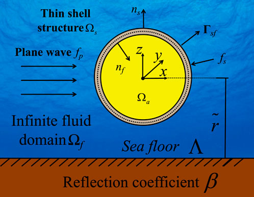
Figure 1. System for acoustic-structural interaction. The unit normal vector of the shell structure is denoted as ${\vec{n}}_s$, while that of the fluid is ${\vec{n}}_f$. A dashed line indicates the mid-surface of the shell structure. The pressure load from the sound field is ${\vec{f}}_p$, and the external mechanical load is ${\vec{f}}_s$.

The mechanical response of the thin-shell is defined by the Kirchhoff-Love shell theory, as detailed in references [36, 37]. Meanwhile, the acoustic fields within the fluid domain are regulated by the Helmholtz equation, which is discussed in [38-41]. The thin-shell structure is actuated by a time-varying force with an angular frequency of $\omega$. Consequently, the equations governing the acoustic-structural interaction system are presented as Equations 1–4.

$\nabla \cdot \mathit{\sigma }\left(\mathbf{x}\right)+{\omega }^2{\rho }_s\mathbf{u}\left(\mathbf{x}\right)=0\mathbf{x}\in {\mathrm{\Omega }}_s(1)$

${\nabla }^{2}p\left(\mathbf{x}\right)+k^{2}p\left(\mathbf{x}\right)=0\mathbf{x}\in {\mathrm{\Omega }}_f(2)$

$\mathit{\sigma }\left(\mathbf{x}\right)\cdot {\mathbf{n}}_s\left(\mathbf{x}\right)-p\left(\mathbf{x}\right){\mathbf{n}}_f\left(\mathbf{x}\right)=0\mathbf{x}\in {\mathrm{\Gamma }}_{sf}(3)$

$-\mathrm{i}\omega \mathbf{u}\left(\mathbf{x}\right)\cdot {\mathbf{n}}_f\left(\mathbf{x}\right)=v_f^n\left(\mathbf{x}\right)\mathbf{x}\in {\mathrm{\Gamma }}_{sf}(4)$

Equations 1, 2 serve as the foundational equations that shape the configuration of acoustic fields. Equations 3, 4 delineate the conditions for continuous displacement and balanced forces at the interfaces where the fluid and structure interact. The symbol $\nabla$ denotes the Laplacian operator, $\mathit{\sigma }$ signifies the stress tensor, $\mathbf{u}$ represents the displacement vector, ${\rho }_s$ is the density of the shell, $p(\mathbf{x})$ denotes the acoustic pressure, ${\mathbf{n}}_s$ is the outward normal vector to the shell surfaces, ${\mathbf{n}}_f$ is the inward normal vector to the structural surface, $\mathrm{i}$ is the imaginary unit with $\mathrm{i}=\sqrt{-1}$, $v_f^n$ is the normal velocity of the fluid, and $k$, defined as $\omega /c$, represents the wave number, with $c$ being the speed of sound propagation within the fluid domain.

2.2 Geometric modeling employing Catmull-Clark subdivision surfaces

The choice of a discretization approach or the selection of basis functions is crucial in numerical simulations. Typically, in traditional FEM and BEM, polynomial functions are the preferred choice for basis functions. In this study, we integrate FEM and BEM within the framework of isogeometric analysis (IGA), as referenced in [42-46]. This integration leverages the same basis functions used for geometric modeling to discretize the physical fields. This approach not only preserves the geometric precision but also eliminates the need for mesh generation. Most significantly, it facilitates the construction of high-order continuous fields, which is essential for the application of the Kirchhoff-Love shell theory, as further elaborated in [47].

Non-Uniform Rational B-splines (NURBS), as discussed in [48- 52], are a prevalent choice for geometric construction in Computer-Aided Design (CAD), with polygonal meshes subsequently derived for numerical analysis. In this research, we embrace the principles of isogeometric analysis, utilizing identical basis functions for both geometric modeling and numerical simulation. We opt for Catmull-Clark subdivision surfaces over NURBS for CAD model construction, as they ensure watertight geometries with support for arbitrary topologies, as described in [53].

Constructing geometry with Catmull-Clark subdivision surfaces begins with the establishment of a control mesh, which is made up of quadrilateral elements. The vertices of this mesh are known as control points. Following the initial setup, the control mesh undergoes subdivision, during which new control points are introduced and the positions of the existing ones are adjusted, as shown in Figure 2. This process of subdivision can be repeated iteratively, adhering to a set of subdivision rules that progress from level $k$ to level $k+1$, as illustrated in Figure 3. However, since continuous subdivision is not feasible, practical implementations of limit subdivision surfaces are assessed through the use of spline basis functions for parameterization.

Figure 2

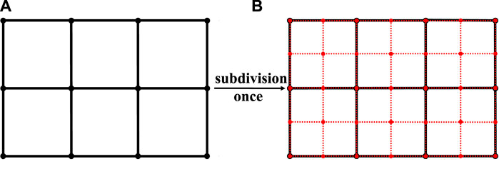
Figure 2. Method for generating Catmull-Clark Subdivision Surfaces. The black points represent the control points prior to subdivision, while the red points indicate the positions after subdivision has been applied. (A) Initial control mesh. (B) One level refined mesh.

Figure 3

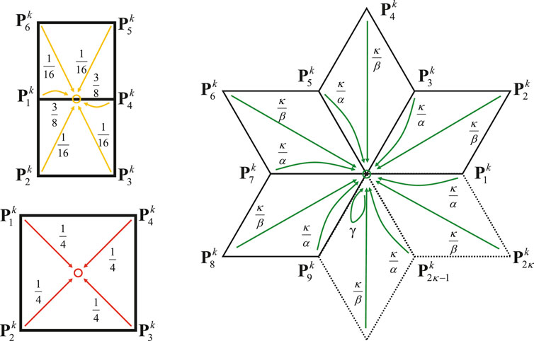
Figure 3. Algorithm pertaining to the topology of Catmull-Clark subdivision surfaces.

Subdivision surfaces excel in their capacity to manage singular points while ensuring controlled curvature at these locations. Figure 4A illustrates a regularly colored subdivision surface element, where each vertex within the element has a valence of 4, signifying the lack of extraordinary vertices within the element. A patch is delineated as a collection of all elements that share vertices with a particular target element. A regular patch is composed of nine elements featuring sixteen vertices. The element highlighted in Figure 4B contains an extraordinary vertex, which adds complexity to surface evaluation as it disrupts the tensor-product property. It should be noted that the initial grid might include irregular elements with multiple extraordinary vertices, but after subdivision, each resulting sub-element will contain at most one exceptional vertex. The evaluation of a surface point with parametric coordinates $(\xi ,\eta )$ is conducted through a linear combination of control points and $2\kappa +8$ basis functions, characterized by a valence of $\kappa$, as shown in Equation 5.

$\mathbf{x}\left(\xi ,\eta \right)={\displaystyle \sum _{\ell =0}^{2\kappa +7}}{\widehat{N}}_{\ell }\left(\xi ,\eta \right){\mathbf{P}}_{\ell }(5)$

in which $\mathbf{x}$ represents the Cartesian coordinates of the point, ${\widehat{N}}_{\ell }$ refers to the basis functions, ${\mathbf{P}}_{\ell }$ signifies the control points, and $\kappa$ indicates the valence of the vertex.

Figure 4

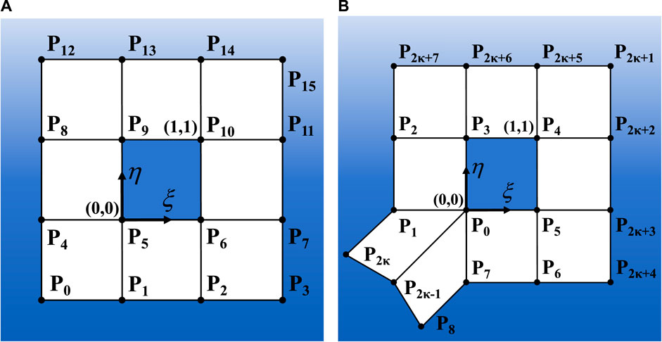
Figure 4. Patches associated with elements in a Catmull-Clark subdivision surface. (A) For a regular element. (B) For an irregular element.

2.3 Analysis of thin-shell vibrations employing IGAFEM

As previously stated, subdivision surfaces are employed for both crafting geometric models and discretizing the physical fields. The collective elements establish the boundary $\mathrm{\Gamma }$, which is delineated by Equation 6.

$\mathrm{\Gamma }={\displaystyle \bigcup _{e=1}^{N_e}}{\mathrm{\Gamma }}_e(6)$

in which $N_e$ denotes the overall count of elements, with element ${\mathrm{\Gamma }}_e$ signifying the $e$-th element. Consequently, the displacement can be articulated as follows by leveraging the basis functions associated with the Catmull-Clark subdivision, as shown in Equation 7.

${\tilde{\mathbf{u}}}^e={\displaystyle \sum _{\ell =0}^{2\kappa +7}}{\widehat{N}}_{\ell }\left(\xi ,\eta \right){\tilde{\mathbf{u}}}_{\ell }^e(7)$

in which ${\tilde{\mathbf{u}}}_{\ell }^e$ denotes the nodal parameter associated with the $\ell$-th control point, employed for discretizing the displacements. Combining all the individual element matrices results in the subsequent Equation 8.

$\mathbf{A}\tilde{\mathbf{u}}=\mathbf{f}(8)$

in which $\tilde{\mathbf{u}}$ represents the vector of displacements at all vertices, and $\mathbf{f}$ signifies the load vector. Furthermore, the matrix $\mathbf{A}$ can be formulated as Equation 9.

$\mathbf{A}=\mathbf{K}-{\omega }^2\mathbf{M},\mathbf{K}={\displaystyle \bigcup _{e=1}^{N_e}}{\mathbf{K}}^e,\mathbf{M}={\displaystyle \bigcup _{e=1}^{N_e}}{\mathbf{M}}^e(9)$

in which $\mathbf{K}$ signifies the global stiffness matrix of the structure, while $\mathbf{M}$ represents the global mass matrix. The element stiffness matrix is denoted by ${\mathbf{K}}^e$ and the element mass matrix by ${\mathbf{M}}^e$. It should be noted that the load vector $\mathbf{f}$ is the sum of two components, ${\mathbf{f}}_s$ and ${\mathbf{f}}_p$, where ${\mathbf{f}}_s$ corresponds to the external mechanical load, and ${\mathbf{f}}_p$ corresponds to the load due to acoustic pressure.

2.4 Analysis of acoustic phenomena employing IGABEM

Within the three-dimensional domain $\mathrm{\Omega }\subset {\mathbb{R}}^3$ bounded by $\mathrm{\Gamma }$, the propagation of acoustic waves is governed by the Helmholtz equation. This equation can be transformed into boundary integral equations. To address the issue of irregular frequencies or spurious modes in exterior acoustic scenarios, we employ the Burton-Miller formulation, which is a linear combination of the conventional boundary integral equation (CBIE) and its derivatives [54-57], as shown in Equation 10.

$\begin{array}{ll}\hfill C\left(\mathbf{x}\right)p\left(\mathbf{x}\right)+\alpha C\left(\mathbf{x}\right)q\left(\mathbf{x}\right)=& {\int }_{\mathrm{\Gamma }}G\left(\mathbf{x},\mathbf{y}\right)q\left(\mathbf{y}\right)\mathrm{d}\mathrm{\Gamma }+\alpha {\int }_{\mathrm{\Gamma }}\frac{\partial G\left(\mathbf{x},\mathbf{y}\right)}{\partial n_f\left(\mathbf{x}\right)}q\left(\mathbf{y}\right)\mathrm{d}\mathrm{\Gamma }\hfill \\ \hfill & -{\int }_{\mathrm{\Gamma }}\frac{\partial G\left(\mathbf{x},\mathbf{y}\right)}{\partial n_f\left(\mathbf{y}\right)}p\left(\mathbf{y}\right)\mathrm{d}\mathrm{\Gamma }\hfill \\ \hfill & -\alpha {\int }_{\mathrm{\Gamma }}\frac{{\partial }^{2}G\left(\mathbf{x},\mathbf{y}\right)}{\partial n_f\left(\mathbf{x}\right)\partial n_f\left(\mathbf{y}\right)}p\left(\mathbf{y}\right)\mathrm{d}\mathrm{\Gamma }+{\tilde{p}}_{\text{inc}}\left(\mathbf{x}\right)\hfill \end{array}(10)$

in which $\mathbf{x}$ and $\mathbf{y}$ correspond to the source and field points, respectively. The term $C(\mathbf{x})$ represents the discontinuity across the boundary, which takes a value of $\frac{1}{2}$ for smooth surfaces. The coupling parameter $\alpha$ is given by $\frac{\text{i}}{k}$ when $k>1$, and $\alpha =\text{i}$ in other cases. The quantity $q(\mathbf{y})=\frac{\partial p(\mathbf{y})}{\partial n_f(\mathbf{y})}$ denotes the flux of sound pressure. The term ${\tilde{p}}_{\text{inc}}(\mathbf{x})=p_{\text{inc}}(\mathbf{x})+\frac{\partial p_{\text{inc}}(\mathbf{x})}{\partial n_f(\mathbf{x})}$ encompasses both the incident wave’s sound pressure and its normal derivative at point $\mathbf{x}$, with $p_{\text{inc}}(\mathbf{x})$ being the incident wave’s sound pressure at that location. The functions $G(\mathbf{x},\mathbf{y})$ and its normal derivative for three-dimensional full-space acoustics are specified as Equations 11, 12.

$G\left(\mathbf{x},\mathbf{y}\right)=\frac{{\text{e}}^{\text{i}kr}}{4\pi r}(11)$

$\frac{\partial G\left(\mathbf{x},\mathbf{y}\right)}{\partial n_f\left(\mathbf{y}\right)}=-\frac{{\text{e}}^{\text{i}kr}}{4\pi r^2}\left(1-\text{i}kr\right)\frac{\partial r}{\partial n_f\left(\mathbf{y}\right)}(12)$

in which $r=|\mathbf{x}-\mathbf{y}|$. The fundamental solution for half-space problems is represented by $G^{*}(\mathbf{x},\mathbf{y})$, as shown in Equation 13.

$G^{*}\left(\mathbf{x},\mathbf{y}\right)=G\left(\mathbf{x},\mathbf{y}\right)+\beta G\left({\mathbf{x}}^{*},\mathbf{y}\right)(13)$

in which $\mathbf{x}*$ denotes the reflection of point $\mathbf{x}$ across the infinite plane ${\mathrm{\Gamma }}_h$, and $\beta$ signifies the reflection coefficient. The coefficient $\beta$ equals one for a rigid boundary and −1 for a soft boundary. By replacing $G(\mathbf{x},\mathbf{y})$ with $G^{*}(\mathbf{x},\mathbf{y})$, Equation 10 is converted into Equation 14.

$\begin{array}{ll}\hfill C\left(\mathbf{x}\right)p\left(\mathbf{x}\right)+\alpha C\left(\mathbf{x}\right)q\left(\mathbf{x}\right)=& {\int }_{\mathrm{\Gamma }}{G}^{*}\left(\mathbf{x},\mathbf{y}\right)q\left(\mathbf{y}\right)\mathrm{d}\mathrm{\Gamma }+\alpha {\int }_{\mathrm{\Gamma }}\frac{\partial G^{*}\left(\mathbf{x},\mathbf{y}\right)}{\partial n_f\left(\mathbf{x}\right)}q\left(\mathbf{y}\right)\mathrm{d}\mathrm{\Gamma }\hfill \\ \hfill & -{\int }_{\mathrm{\Gamma }}\frac{\partial G^{*}\left(\mathbf{x},\mathbf{y}\right)}{\partial n_f\left(\mathbf{y}\right)}p\left(\mathbf{y}\right)\mathrm{d}\mathrm{\Gamma }\hfill \\ \hfill & -\alpha {\int }_{\mathrm{\Gamma }}\frac{{\partial }^2{G}^{*}\left(\mathbf{x},\mathbf{y}\right)}{\partial n_f\left(\mathbf{x}\right)\partial n_f\left(\mathbf{y}\right)}p\left(\mathbf{y}\right)\mathrm{d}\mathrm{\Gamma }+{\tilde{p}}_{\text{inc}}^{*}\left(\mathbf{x}\right)\hfill \end{array}(14)$

in which ${\tilde{p}}_{\text{inc}}^{*}(\mathbf{x})=p_{\text{inc}}^{*}(\mathbf{x})+\frac{\partial p_{\text{inc}}^{*}(\mathbf{x})}{\partial n_f(\mathbf{x})}$, and the partial derivative of G*(x,y) is shown in Equations 15–17.

$\frac{\partial G^{*}\left(\mathbf{x},\mathbf{y}\right)}{\partial n_f\left(\mathbf{y}\right)}=-\frac{{\text{e}}^{\text{i}kr}}{4\pi r^2}\left(1-\text{i}kr\right)\frac{\partial r}{\partial n_f\left(\mathbf{y}\right)}-\beta \frac{{\text{e}}^{\text{i}k{r}^{*}}}{4\pi {\left(r^{*}\right)}^2}\left(1-\text{i}k{r}^{*}\right)\frac{\partial r^{*}}{\partial n_f\left(\mathbf{y}\right)}(15)$

$\frac{\partial G^{*}\left(\mathbf{x},\mathbf{y}\right)}{\partial n_f\left(\mathbf{x}\right)}=-\frac{{\text{e}}^{\text{i}kr}}{4\pi r^2}\left(1-\text{i}kr\right)\frac{\partial r}{\partial n_f\left(\mathbf{x}\right)}-\beta \frac{{\text{e}}^{\text{i}k{r}^{*}}}{4\pi {\left(r^{*}\right)}^2}\left(1-\text{i}k{r}^{*}\right)\frac{\partial r^{*}}{\partial n_f\left(\mathbf{x}\right)}(16)$

$\begin{array}{l}\frac{{\partial }^2{G}^{*}\left(\mathbf{x},\mathbf{y}\right)}{\partial n_f\left(\mathbf{x}\right)\partial n_f\left(\mathbf{y}\right)}=\frac{{\text{e}}^{\text{i}kr}}{4\pi r^3}\left[\left(3-3\text{i}kr-k^2{r}^2\right)\frac{\partial r}{\partial n_f\left(\mathbf{y}\right)}\frac{\partial r}{\partial n_f\left(\mathbf{x}\right)}+\left(1-\mathrm{i}kr\right)n_i\left(\mathbf{x}\right)n_i\left(\mathbf{y}\right)\right]\hfill \\ \hfill & +\beta \frac{{\text{e}}^{\text{i}k{r}^{*}}}{4\pi {\left(r^{*}\right)}^3}\left[\left(3-3\text{i}k{r}^{*}-k^2{\left(r^{*}\right)}^2\right)\frac{\partial r}{\partial n_f\left(\mathbf{y}\right)}\frac{\partial r}{\partial n_f\left(\mathbf{x}\right)}\right.\hfill \\ \hfill & \left.+\left(1-\mathrm{i}k{r}^{*}\right)n_i\left(\mathbf{x}\right)n_i\left(\mathbf{y}\right)\right]\hfill \end{array}(17)$

In this approach, the physical field is discretized using the basis functions of the subdivision surface that are employed in the geometric construction, as displayed in Equation 18.

$\begin{array}{ll}\hfill & p_e={\displaystyle \sum _{\ell =0}^{2\kappa +7}}{\widehat{N}}_{\ell }\left(\xi ,\eta \right){\tilde{p}}_{\ell }^e\hfill \\ \hfill & q_e={\displaystyle \sum _{\ell =0}^{2\kappa +7}}{\widehat{N}}_{\ell }\left(\xi ,\eta \right){\tilde{q}}_{\ell }^e\hfill \end{array}(18)$

in which $p_e$ represents the acoustic pressure at the point $(\xi ,\eta )$ within the element ${\mathrm{\Gamma }}_e$; $q_e$ signifies the normal flux associated with $p_e$. Additionally, ${\tilde{p}}_{\ell }^e$ refers to the $\ell$-th nodal variable associated with the sound pressure, while ${\tilde{q}}_{\ell }^e$ represents the normal flux corresponding to ${\tilde{p}}_{\ell }^e$. By inserting Equation 18 into Equation 14 and applying these equations at a discrete set of collocation points ${\mathbf{x}}_j$, Equation 19 can be derived.

$\begin{array}{ll}\hfill & C\left({\mathbf{x}}_j\right)p\left({\mathbf{x}}_j\right)+\alpha C\left({\mathbf{x}}_j\right)q\left({\mathbf{x}}_j\right)+{\displaystyle \sum _{e=1}^{N_e}}{\displaystyle \sum _{\ell =0}^{2\kappa +7}}{\int }_{{\mathrm{\Gamma }}_e}{\widehat{N}}_{\ell }\left(\xi ,\eta \right)\frac{\partial G^{*}\left({\mathbf{x}}_j,\mathbf{y}\left(\xi ,\eta \right)\right)}{\partial n_f\left(\mathbf{y}\left(\xi ,\eta \right)\right)}\mathrm{d}\mathrm{\Gamma }{\tilde{p}}_{\ell }^e\hfill \\ \hfill & +\alpha {\displaystyle \sum _{e=1}^{N_e}}{\displaystyle \sum _{\ell =0}^{2\kappa +7}}{\int }_{{\mathrm{\Gamma }}_e}{\widehat{N}}_{\ell }\left(\xi ,\eta \right)\frac{{\partial }^2{G}^{*}\left({\mathbf{x}}_j,\mathbf{y}\left(\xi ,\eta \right)\right)}{\partial n_f\left({\mathbf{x}}_j\right)\partial n_f\left(\mathbf{y}\left(\xi ,\eta \right)\right)}\mathrm{d}\mathrm{\Gamma }{\tilde{p}}_{\ell }^e\hfill \\ \hfill & ={\displaystyle \sum _{e=1}^{N_e}}{\displaystyle \sum _{\ell =0}^{2\kappa +7}}{\int }_{{\mathrm{\Gamma }}_e}{\widehat{N}}_{\ell }\left(\xi ,\eta \right)G^{*}\left({\mathbf{x}}_j,\mathbf{y}\left(\xi ,\eta \right)\right)\mathrm{d}\mathrm{\Gamma }{\tilde{q}}_{\ell }^e\hfill \\ \hfill & +\alpha {\displaystyle \sum _{e=1}^{N_e}}{\displaystyle \sum _{\ell =0}^{2\kappa +7}}{\int }_{{\mathrm{\Gamma }}_e}{\widehat{N}}_{\ell }\left(\xi ,\eta \right)\frac{\partial G^{*}\left({\mathbf{x}}_j,\mathbf{y}\left(\xi ,\eta \right)\right)}{\partial n_f\left({\mathbf{x}}_j\right)}\mathrm{d}\mathrm{\Gamma }{\tilde{q}}_{\ell }^e+{\tilde{p}}_{\text{inc}}^{*}\left({\mathbf{x}}_j\right)\hfill \end{array}(19)$

in which the subscript $j$ indicates the index of the collocation point. These collocation points are determined by projecting the control points onto the surface. Equation 19 can be expressed in matrix-vector form as Equation 20.

$\mathbf{H}\tilde{\mathbf{p}}=\mathbf{G}\tilde{\mathbf{q}}+{\mathbf{p}}_{\mathbf{i}}(20)$

in whichn $\mathbf{H}$ and $\mathbf{G}$ are the matrices of coefficients, while $\tilde{\mathbf{p}}$ and $\tilde{\mathbf{q}}$ are the column vectors that compile the nodal parameters related to the acoustic pressure and its flux, respectively. ${\mathbf{p}}_{\mathbf{i}}$ signifies the nodal pressure vector attributed to the incident wave. It is crucial to address the singular integrals present in Equation 10. Numerous methods have been proposed to handle these singular integrals within BEM, as cited in [58-61]. This research adopts the singularity subtraction technique introduced by Guiggiani, recognized for its precision and efficiency, as detailed in [62].

2.5 Integration of IGAFEM and IGABEM

Equations 8, 20, originating from the structure (using FEM) and the acoustic (using BEM) respectively, are tightly interlinked and cannot be resolved in isolation. They are interconnected through the boundary conditions outlined in Equations 3, 4. The sound pressure within the fluid domain can be perceived as a force exerted on the shell surface. Consequently, the nodal force vector ${\mathbf{f}}_p$ due to the acoustic load can be formulated as Equation 21.

${\mathbf{f}}_p={\tilde{\mathbf{n}}}_f\mathrm{\Theta }\tilde{\mathbf{p}}(21)$

in which $\mathrm{\Theta }$ is defined as the integral over the boundary $\mathrm{\Gamma }$ of the product of the transpose of the subdivision basis functions’ global vector ${\widehat{N}}_{\ell }$ and ${\widehat{N}}_{\ell }$ itself, multiplied by $d\mathrm{\Gamma }$. The vector ${\widehat{N}}_{\ell }$ denotes the global vector of subdivision basis functions, and ${\tilde{\mathbf{n}}}_f$ represents the matrix of normal vectors, which is given by Equation 22.

${\tilde{\mathbf{n}}}_f=\left\{\begin{array}{c}{n}_{1f}\cdot e_1\text{0\hspace{0.17em}}\dots \hfill \\ n_{1f}\cdot e_2\text{0\hspace{0.17em}}\dots \hfill \\ n_{1f}\cdot e_3\text{0\hspace{0.17em}}\dots \hfill \\ \text{0\hspace{0.17em}}{n}_{2f}\cdot e_1\dots \hfill \\ \text{0\hspace{0.17em}}{n}_{2f}\cdot e_2\dots \hfill \\ \text{0\hspace{0.17em}}{n}_{2f}\cdot e_3\dots \hfill \\ \dots \dots \dots \hfill \end{array}\right\}(22)$

in which $e_1,e_2,e_3$ denote the three unit normal vectors. By applying Equation 21, we can derive a new expression for the global nodal force vector, which is presented in Equation 23.

$\mathbf{f}={\mathbf{C}}_{sf}\tilde{\mathbf{p}}+{\mathbf{f}}_s(23)$

in which ${\mathbf{C}}_{sf}={\tilde{\mathbf{n}}}_f\mathrm{\Theta }$.

Next, we will investigate the relationship between the velocities on the shell’s mid-surface and the sound pressure. The vector ${\mathbf{v}}_f^n$ represents the nodal parameters related to the fluid’s normal velocity component, while the vector ${\mathbf{v}}_s^n$ signifies the nodal variables associated with the normal velocity component of the structure. Assuming no energy dissipation occurs at the interface between the fluid and structural domains, we get Equation 24.

${\mathbf{v}}_f^n-{\mathbf{v}}_s^n=0(24)$

in which ${\mathbf{v}}_s^n=\mathrm{i}\omega {\mathbf{C}}_{fs}\tilde{\mathbf{u}}$, and ${\mathbf{C}}_{fs}={\tilde{\mathbf{n}}}_f^{\text{T}}$. Subsequently, the vector $\tilde{\mathbf{q}}$, encompassing the nodal parameters related to the acoustic flux, can be formulated as Equation 25.

$\tilde{\mathbf{q}}=\frac{\partial \tilde{\mathbf{p}}}{\partial n}=-\mathrm{i}\omega {\rho }_f{\mathbf{v}}_f^n={\omega }^2{\rho }_f{\mathbf{C}}_{fs}\tilde{\mathbf{u}}(25)$

in which ${\rho }_f$ represents the fluid’s density.

By inserting Equation 25 into Equation 20, we obtain the following coupled system of equations for the acoustics, as shown in Equation 26.

$\mathbf{H}\tilde{\mathbf{p}}=\mathbf{G}{\omega }^2{\rho }_f{\mathbf{C}}_{fs}\tilde{\mathbf{u}}+{\mathbf{p}}_{\mathbf{i}}(26)$

Incorporating Equation 23 into Equation 8 yields the following coupled system of equations for structural dynamics shown in Equation 27.

$\mathbf{A}\tilde{\mathbf{u}}={\mathbf{C}}_{sf}\tilde{\mathbf{p}}+{\mathbf{f}}_s(27)$

By integrating Equation 27 into Equation 26, the indeterminate displacement $\tilde{\mathbf{u}}$ is eliminated, leading to a boundary element formulation that is linked with the finite element equation, as shown in Equation 28.

$\left[\mathbf{H}-\mathbf{G}\mathbf{Y}\right]\tilde{\mathbf{p}}={\mathbf{G}\tilde{\mathbf{q}}}_s+{\mathbf{p}}_{\mathbf{i}}(28)$

in which $\mathbf{Y}$ denotes the global admittance matrix, and ${\tilde{\mathbf{q}}}_s$ accounts for the influence of sound speeds originating from the structural domain. These are given by Equation 29.

$\begin{array}{ll}\hfill & \mathbf{Y}={\omega }^2{\rho }_f{\mathbf{C}}_{fs}{\mathbf{A}}^{-1}{\mathbf{C}}_{sf}\hfill \\ \hfill & {\tilde{\mathbf{q}}}_s={\omega }^2{\rho }_f{\mathbf{C}}_{fs}{\mathbf{A}}^{-1}{\mathbf{f}}_s\hfill \end{array}(29)$

3 Enhancing computation speed with the fast multipole method

The Fast Multipole Method (FMM) is a highly efficient algorithm designed to accelerate the computation of long-range interactions in N-body problems. Introduced by [63], FMM reduces the computational complexity from $\mathcal{O}(N^2)$ to $\mathcal{O}(N)$ or $\mathcal{O}(N\log N)$, depending on the implementation. This significant improvement is achieved through hierarchical space decomposition and the use of multipole and local expansions, which approximate interactions between distant clusters of particles. The fundamental solution for the full-space, as introduced in Equation 11, is expanded into the following series shown in Equation 30.

$G(\mathbf{x},\mathbf{y})=\frac{\text{i}k}{4\pi }{\displaystyle \sum _{n=0}^{\infty }}{\displaystyle \sum _{m=-n}^n}\left(2n+1\right){\bar{\mathbf{I}}}_n^m\left(k,\overrightarrow{\mathbf{o}\mathbf{y}}\right){\mathbf{O}}_n^m\left(k,\overrightarrow{\mathbf{o}\mathbf{x}}\right)(30)$

in which $\mathbf{O}$ serves as a local expansion point in proximity to $\mathbf{y}$, as shown in Figure 5. The terms ${\mathbf{I}}_n^m$ and ${\mathbf{O}}_n^m$ are defined as Equations 31, 32.

${\mathbf{I}}_n^m\left(k,a\right)=j_n\left(kr\right){\mathbf{Y}}_n^m\left(\theta ,\varphi \right)(31)$

${\mathbf{O}}_n^m\left(k,a\right)=h_n^{\left(1\right)}\left(kr\right){\mathbf{Y}}_n^m\left(\theta ,\varphi \right)(32)$

The terms ${\bar{\mathbf{I}}}_n^m$ represent the complex conjugates of ${\mathbf{I}}_n^m$. The functions $j_n$ and $h_n^{(1)}$ correspond to the $n$-th order spherical Bessel and Hankel functions of the first kind, respectively, as detailed in [64]. The spherical harmonics are denoted by ${\mathbf{Y}}_n^m$, which are given by Equation 33.

${\mathbf{Y}}_n^m\left(\theta ,\varphi \right)=c_n^m{\mathbf{P}}_n^m\left(\cos \theta \right)e^{im\varphi }(33)$

in which $c_n^m=\sqrt{\frac{(n-m)!}{(n+m)!}}$ and ${\mathbf{P}}_n^m$ refers to the associated Legendre functions.

Figure 5

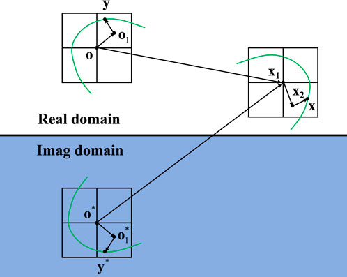
Figure 5. Nodes at the boundary and the points for multipole expansion in the half-space Fast Multipole Method (FMM).

To derive a Fast Multipole Method (FMM) scheme tailored for a half-space acoustic problem, we modify the fundamental solution for the half-space into the following form in Equation 34.

$G^{*}\left(\mathbf{x},\mathbf{y}\right)=G\left(\mathbf{x},\mathbf{y}\right)+\beta G\left(\mathbf{x},{\mathbf{y}}^{*}\right)(34)$

Subsequently, the boundary integral for the $j$-th element in Equation 28 can be re-expressed as Equations 35, 36.

$g^{ij}={\int }_{{\mathrm{\Gamma }}_j}\left.G(\mathbf{x},\mathbf{y})+\beta G(\mathbf{x},{\mathbf{y}}^{*})\right]q\left(\mathbf{y}\right)d\mathrm{\Gamma }\left(\mathbf{y}\right)(35)$

$h^{ij}={\int }_{{\mathrm{\Gamma }}_j}\left[\frac{\partial G(\mathbf{x},\mathbf{y})}{\partial n_f\left(\mathbf{y}\right)}+\beta \frac{\partial G(\mathbf{x},{\mathbf{y}}^{*})}{\partial n_f\left(\mathbf{y}\right)}\right]p\left(\mathbf{y}\right)d\mathrm{\Gamma }\left(\mathbf{y}\right)(36)$

Consequently, employing Equation 13, we can express the boundary integrals over a boundary element ${\mathrm{\Gamma }}_j$ that is situated at a distance from the source point $\mathbf{x}$ in the following manner in Equations 37, 38.

$g^{ij}=\frac{ik}{4\pi }{\displaystyle \sum _{n=0}^{\infty }}{\displaystyle \sum _{m=-n}^n}\left(2n+1\right)\left[{\mathbf{M}}_n^m\left(k,{\overrightarrow{\mathbf{o}\mathbf{y}}}_j\right){\mathbf{O}}_n^m\left(k,\overrightarrow{\mathbf{o}\mathbf{x}}\right)+\beta {\mathbf{M}}_n^m\left(k,\overrightarrow{{\mathbf{o}}^{*}{\mathbf{y}}_j^{*}}\right){\mathbf{O}}_n^m\left(k,\overrightarrow{{\mathbf{o}}^{*}\mathbf{x}}\right)\right](37)$

$h^{ij}=\frac{ik}{4\pi }{\displaystyle \sum _{n=0}^{\infty }}{\displaystyle \sum _{m=-n}^n}\left(2n+1\right)\left[{\tilde{\mathbf{M}}}_n^m\left(k,\overrightarrow{{\mathbf{o}\mathbf{y}}_j}\right){\mathbf{O}}_n^m\left(k,\overrightarrow{\mathbf{o}\mathbf{x}}\right)+\beta {\tilde{\mathbf{M}}}_n^m\left(k,\overrightarrow{{\mathbf{o}}^{*}{\mathbf{y}}_j^{*}}\right){\mathbf{O}}_n^m\left(k,\overrightarrow{{\mathbf{o}}^{*}\mathbf{x}}\right)\right](38)$

in which ${\mathbf{y}}_j$ denotes a field point on ${\mathrm{\Gamma }}_j$; ${\mathbf{M}}_n^m(k,\overrightarrow{{\mathbf{o}\mathbf{y}}_j})$ and ${\tilde{\mathbf{M}}}_n^m(k,\overrightarrow{{\mathbf{o}\mathbf{y}}_j})$ are the multipole moments of the low-frequency FMM techniques in the real domain, respectively, and are defined as Equations 39, 40.

${\mathbf{M}}_n^m\left(k,\overrightarrow{{\mathbf{o}\mathbf{y}}_j}\right)={\int }_{{\mathrm{\Gamma }}_j}{\bar{\mathbf{I}}}_n^m\left(k,\overrightarrow{{\mathbf{o}\mathbf{y}}_j}\right)q\left(\mathbf{y}\right)d\mathrm{\Gamma }\left(\mathbf{y}\right)(39)$

${\tilde{\mathbf{M}}}_n^m\left(k,\overrightarrow{{\mathbf{o}\mathbf{y}}_j}\right)={\int }_{{\mathrm{\Gamma }}_j}\frac{\partial {\bar{\mathbf{I}}}_n^m\left(k,\overrightarrow{{\mathbf{o}\mathbf{y}}_j}\right)}{\partial n\left(\mathbf{y}\right)}p\left(\mathbf{y}\right)d\mathrm{\Gamma }\left(\mathbf{y}\right)(40)$

By replacing $\mathbf{o}$ and ${\mathbf{y}}_j$ with $\mathbf{o}*$ and ${\mathbf{y}*}_j$ in Equations 39, 40, we obtain the expressions for ${\mathbf{M}}_n^m(k,\overrightarrow{{\mathbf{o}}^{*}{\mathbf{y}*}_j})$ and ${\tilde{\mathbf{M}}}_n^m(k,\overrightarrow{{\mathbf{o}}^{*}{\mathbf{y}*}_j})$ as presented in Equations 37, 38, respectively. To determine the moments of the leaf cell, we aggregate the multipole moments from $N_l$ boundary elements in the vicinity of point $\mathbf{o}$, as shown in Equations 41–44.

${\mathbf{M}}_n^m\left(k,\mathbf{o}\right)={\displaystyle \sum _{j=1}^{N_l}}{\mathbf{M}}_n^m\left(k,\overrightarrow{\mathbf{o}{\mathbf{y}}_j}\right)(41)$

${\mathbf{M}}_n^m\left(k,{\mathbf{o}}^{*}\right)={\displaystyle \sum _{j=1}^{N_l}}{\mathbf{M}}_n^m\left(k,\overrightarrow{{\mathbf{o}}^{*}{\mathbf{y}}_j^{*}}\right)(42)$

${\tilde{\mathbf{M}}}_n^m\left(k,\mathbf{o}\right)={\displaystyle \sum _{j=1}^{N_l}}{\tilde{\mathbf{M}}}_n^m\left(k,\overrightarrow{\mathbf{o}{\mathbf{y}}_j}\right)(43)$

${\tilde{\mathbf{M}}}_n^m\left(k,{\mathbf{o}}^{*}\right)={\displaystyle \sum _{j=1}^{N_l}}{\tilde{\mathbf{M}}}_n^m\left(k,\overrightarrow{{\mathbf{o}}^{*}{\mathbf{y}}_j^{*}}\right)(44)$

When $|{\mathbf{o}}_1\mathbf{x}|>|{\mathbf{o}}_1\mathbf{y}|$ and $|{\mathbf{o}*}_1\mathbf{x}|>|{\mathbf{o}*}_1\mathbf{y}*|$, the low-frequency Fast Multipole Method (FMM) facilitates the relocation of the moment center from $\mathbf{o}$ and $\mathbf{o}*$ to ${\mathbf{o}}_1$ and ${\mathbf{o}*}_1$ using the M2M (moments to moments) translation formula, which is expressed as Equations 45, 46.

${\mathbf{M}}_n^m\left(k,{\mathbf{o}}_1\right)={\displaystyle \sum _{n_1=0}^{\infty }}{\displaystyle \sum _{m_1=-n_1}^{n_1}}{\displaystyle \sum _{l\in \mathfrak{I}}}\left(2n_1+1\right){\left(-1\right)}^{m_1}{W}_{n,n_1,m,m_1,l}\times I_l^{-m-m_1}\left(k,\overrightarrow{{\mathbf{o}}_{\mathbf{1}}\mathbf{o}}\right)(45)$

${\mathbf{M}}_n^m\left(k,{\mathbf{o}}_1^{*}\right)={\displaystyle \sum _{n_1=0}^{\infty }}{\displaystyle \sum _{m_1=-n_1}^{n_1}}{\displaystyle \sum _{l\in \mathfrak{I}}}\left(2n_1+1\right){\left(-1\right)}^{m_1}{W}_{n,n_1,m,m_1,l}\times I_l^{-m-m_1}\left(k,\overrightarrow{{\mathbf{o}}_{\mathbf{1}}^{*}{\mathbf{o}}^{*}}\right)(46)$

in which $W_{n,n_1,m,m_1,l}$ is expressed in Equation 47.

$W_{n,n_1,m,m_1,l}=\left(2l+1\right){\text{i}}^{n_1-n+l}\left(\begin{array}{c}\hfill n{n}_{1}l\hfill \\ \hfill 000\hfill \end{array}\right)\left(\begin{array}{c}\hfill n{n}_{1}l\hfill \\ \hfill m{m}_1-m-m_1\hfill \end{array}\right)(47)$

The symbol $\left(\begin{array}{c}\hfill .\hfill \\ \hfill .\hfill \end{array}\right)$ represents the Wigner 3j symbol, and the set $\mathfrak{I}$ is defined as Equation 48.

$\mathfrak{I}\left(n,n_1,m,m_1\right)=\left\{\begin{array}{c}l|l\in \mathbf{Z},n+n_1-l:even,\hfill \\ \max \left\{\left|m+m_1\right|,\left|n-n_1\right|\right\}\le l\le n+n_1\hfill \end{array}\right\}(48)$

Taking into account the influence of the infinite/symmetry plane, we can formulate the M2L (moments to local expansion coefficients) translation formula as shown in Equations 49, 50.

$\begin{array}{ll}\hfill L_n^m\left(k,{\mathbf{x}}_1\right)& ={\displaystyle \sum _{n_1=0}^{\infty }}{\displaystyle \sum _{m_1=-n_1}^{n_1}}{\displaystyle \sum _{l\in \mathfrak{I}}}\left(2n_1+1\right){\left(-1\right)}^{m_1}{W}_{n,n_1,m,m_1,l}\hfill \\ \hfill & \times \left[{\mathbf{O}}_l^{m+m_1}\left(k,\overrightarrow{{\mathbf{o}}_1{\mathbf{x}}_1}\right){\mathbf{M}}_{n_1}^{m_1}\left(k,{\mathbf{o}}_1\right)+\beta {\mathbf{O}}_l^{m+m_1}\left(k,\overrightarrow{{\mathbf{o}}_{\mathbf{1}}{\mathbf{x}}_{\mathbf{1}}}\right){\mathbf{M}}_{n_1}^{m_1}\left(k,{\mathbf{o}}_1^{*}\right)\right]\hfill \end{array}(49)$

$\begin{array}{ll}\hfill {\tilde{L}}_n^m\left(k,{\mathbf{x}}_1\right)& ={\displaystyle \sum _{n_1=0}^{\infty }}{\displaystyle \sum _{m_1=-n_1}^{n_1}}{\displaystyle \sum _{l\in \mathfrak{I}}}\left(2n_1+1\right){\left(-1\right)}^{m_1}{W}_{n,n_1,m,m_1,l}\hfill \\ \hfill & \times \left[{\mathbf{O}}_l^{m+m_1}\left(k,\overrightarrow{{\mathbf{o}}_1{\mathbf{x}}_1}\right){\tilde{M}}_{n_1}^{m_1}\left(k,{\mathbf{o}}_1\right)+\beta {\mathbf{O}}_l^{m+m_1}\left(k,\overrightarrow{{\mathbf{o}}_1{\mathbf{x}}_1}\right){\tilde{M}}_{n_1}^{m_1}\left(k,{\mathbf{o}}_1^{*}\right)\right]\hfill \end{array}(50)$

Following that, the L2L (local expansion to local expansion) translation formula can be employed to shift the center of the local expansion from ${\mathbf{x}}_1$ to ${\mathbf{x}}_2$, as shown in Equations 51, 52.

$\begin{array}{ll}\hfill L_n^m\left(k,{\mathbf{x}}_2\right)& ={\displaystyle \sum _{n_1=0}^{\infty }}{\displaystyle \sum _{m_1=-n_1}^{n_1}}{\displaystyle \sum _{l\in \mathfrak{I}}}\left(2n_1+1\right){\left(-1\right)}^{m_1}{W}_{n,n_1,-m,m_1,l}\hfill \\ \hfill & \times I_l^{m-m_1}\left(k,\overrightarrow{{\mathbf{x}}_1{\mathbf{x}}_2}\right)L_{n_1}^{m_1}\left(k,{\mathbf{x}}_1\right)\hfill \end{array}(51)$

$\begin{array}{ll}\hfill {\tilde{L}}_n^m\left(k,{\mathbf{x}}_2\right)& ={\displaystyle \sum _{n_1=0}^{\infty }}{\displaystyle \sum _{m_1=-n_1}^{n_1}}{\displaystyle \sum _{l\in \mathfrak{I}}}\left(2n_1+1\right){\left(-1\right)}^{m_1}{W}_{n,n_1,-m,m_1,l}\hfill \\ \hfill & \times I_l^{m-m_1}\left(k,\overrightarrow{{\mathbf{x}}_1{\mathbf{x}}_2}\right){\tilde{L}}_{n_1}^{m_1}\left(k,{\mathbf{x}}_1\right)\hfill \end{array}(52)$

For the set of $N_l$ boundary elements that are close to $\mathbf{o}$ but far from the source points $\mathbf{x}$, the sums ${\sum }_{j=1}^{N_l}{h}^{ij}$ or ${\sum }_{j=1}^{N_l}{g}^{ij}$ can be expressed using the local expansion coefficients shown in Equation 53.

${\displaystyle \sum _{j=1}^{N_l}}{g}^{ij}=\frac{\text{i}k}{4\pi }{\displaystyle \sum _{n=0}^{\infty }}{\displaystyle \sum _{m=-n}^n}\left(2n+1\right)L_n^m\left(k,{\mathbf{x}}_2\right){\bar{I}}_n^m\left(k,\overrightarrow{{\mathbf{x}}_2{\mathbf{x}}_1}\right)(53)$

${\displaystyle \sum _{j=1}^{N_l}}{h}^{ij}=\frac{\text{i}k}{4\pi }{\displaystyle \sum _{n=0}^{\infty }}{\displaystyle \sum _{m=-n}^n}\left(2n+1\right){\tilde{L}}_n^m\left(k,{\mathbf{x}}_2\right){\bar{I}}_n^m\left(k,\overrightarrow{{\mathbf{x}}_2{\mathbf{x}}_1}\right)(54)$

within the low-frequency FMM. To refine the Burton-Miller formulation, which is a linear combination of the Conventional Boundary Integral Equation (CBIE) and its normal derivative, we simply introduce adjustments to Equations 53, 54, as shown in Equations 55, 56.

${\displaystyle \sum _{j=1}^{N_l}}{g}^{ij}=\frac{\text{i}k}{4\pi }{\displaystyle \sum _{n=0}^{\infty }}{\displaystyle \sum _{m=-n}^n}\left(2n+1\right)L_n^m\left(k,{\mathbf{x}}_2\right)\times \left[{\bar{I}}_n^m\left(k,\overrightarrow{{\mathbf{x}}_2{\mathbf{x}}_1}\right)+\alpha \frac{\partial {\bar{I}}_n^m\left(k,\overrightarrow{{\mathbf{x}}_2{\mathbf{x}}_1}\right)}{\partial n\left(\mathbf{x}\right)}\right](55)$

${\displaystyle \sum _{j=1}^{N_l}}{h}^{ij}=\frac{\text{i}k}{4\pi }{\displaystyle \sum _{n=0}^{\infty }}{\displaystyle \sum _{m=-n}^n}\left(2n+1\right){\tilde{L}}_n^m\left(k,{\mathbf{x}}_2\right)\times \left[{\bar{I}}_n^m\left(k,\overrightarrow{{\mathbf{x}}_2{\mathbf{x}}_1}\right)+\alpha \frac{\partial {\bar{I}}_n^m\left(k,\overrightarrow{{\mathbf{x}}_2{\mathbf{x}}_1}\right)}{\partial n\left(\mathbf{x}\right)}\right](56)$

The implementation process involves the following key steps:

1. Hierarchical Tree Construction: The computational domain is partitioned into a hierarchical octree structure, with each node representing a subdomain. Boundary elements are assigned to the appropriate nodes based on their spatial location.

2. Multipole Expansion Calculation: For each leaf node, multipole moments are computed using the source terms within the node. These moments encapsulate the collective influence of sources on distant targets.

3. M2M Translations: Multipole expansions from child nodes are aggregated and translated to their parent nodes, propagating the influence up the hierarchical tree.

4. M2L Translations: At each interaction list, multipole expansions from distant nodes are translated into local expansions at the target nodes. This step leverages the translation operators to approximate interactions efficiently.

5. L2L Translations: Local expansions are propagated down the tree to account for interactions within localized regions.

6. Evaluation of Local Expansions: The final local expansions are evaluated at the target points, providing the approximate contributions from distant sources.

4 Numerical illustrations

In this segment, the primary objective of the elastic spherical shell model is to verify the accuracy of the numerical model by comparing the analytical and numerical solutions. The fish model, with its relatively complex geometry, represents the structural features of real underwater organisms or submersibles. It is intended to demonstrate the applicability and effectiveness of the proposed method in solving underwater acoustic scattering problems. The computations are executed using Fortran 90 on a desktop computer with 128 GB of RAM and an Intel (R) Core (TM) i7-7700 CPU.

4.1 Acoustic scattering by an elastic spherical shell

This section examines the acoustic field scattered by a spherical shell structure when subjected to incident plane waves, taking into account the reflections from the seabed, as depicted in Figure 6. In the diagram, the center of the sphere is at the origin; $\mathrm{\Lambda }$ represents the seabed surface; $\tilde{r}$ is the distance from the origin to the seabed surface; $f_p$ is the incident plane wave; ${\mathrm{\Omega }}_f$ signifies the infinite fluid domain. The seabed reflection coefficient is denoted by $\beta$, where $\beta =-1$ corresponds to a soft seabed and $\beta =1$ corresponds to a rigid seabed.The incident plane waves, which have an amplitude of 1, travel along the positive $x$-axis. Using Catmull-Clark subdivision surfaces, three elastic spherical shells with 3,458, 4,800, and 9,408 mesh points were constructed. Figure 7 presents the variation curves of sound pressure with frequency for the spherical models at 3,458, 4,800, and 9,408 mesh points, respectively. The computation times for a single frequency were 33 s, 56 s, and 85 s for each model. It can be observed from the figure that the differences in the sound pressure curves across the three mesh densities are minimal; however, the computation times differ significantly. Therefore, this study adopts the spherical model with fewer mesh points to balance computational efficiency and accuracy.When analyzing the acoustic scattering of the sphere model, we found that the computation time for the traditional Catmull-Clark subdivision surfaces coupled with the FEM-BEM method was 428 s, whereas the computation time for the Catmull-Clark subdivision surfaces accelerated by FMM and coupled with the FEM-BEM method was only 33 s, demonstrating that the computational efficiency of FMM is significantly higher than that of traditional algorithms.

Figure 6

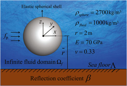
Figure 6. System for acoustic-structural interaction involving elastic spherical shells.

Figure 7

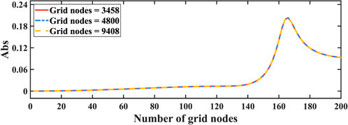
Figure 7. The numerical results of the sphere model are verified in the convergence of three mesh node numbers.

The sound pressure values at the computed points on the circle for incident wave frequencies of 100 Hz and 200 Hz are depicted in Figure 8, where the circle represents the projection of the sphere model, with a radius of 2 m, onto the $yoz$ plane. As observed in the figure, at a frequency of 200 Hz, the sound pressure curve exhibits more pronounced fluctuations, indicating that the larger the external sound wave impacting the sphere model, the greater the magnitude of sound pressure variation. When $\beta =0$, the sound pressure curves from numerical and analytical solutions align, confirming the validity and reliability of the algorithm presented in this study. For $\beta =\mathrm{0,1},-1$, the numerical solutions vary significantly, demonstrating the importance of considering the seabed reflection effects and highlighting the significance of the seabed’s nature.

Figure 8

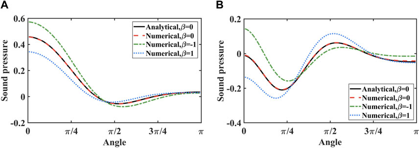
Figure 8. Sound pressure at computational points on circles with a 2-m radius across various frequencies. (A) 100 Hz. (B) 200 Hz.

Figure 9 illustrates the displacement and sound pressure distributions on the sphere model when it is positioned 5 m above the seabed. The first three columns represent the displacement components in the $x$, $y$, and $z$ axes, respectively, while the last column indicates the sound pressure. As observed in the figure, the sound pressure pattern exhibits symmetry along the $x$-axis, and the displacement components also mirror this symmetry. The displacement in the $x$-direction is the most significant, whereas the $y$-direction shows the least. The sound pressure on the sphere’s surface diminishes as we move in the negative $x$-axis direction, whereas the $x$-direction displacement component increases progressively.

Figure 9

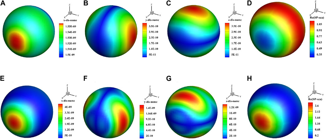
Figure 9. Sound pressure and displacement distributions on the surface of a spherical shell: the first three columns depict the three components of displacement, while the fourth column shows the sound pressure. (A) 100 Hz, displacement x. (B) 100 Hz, displacement y. (C) 100 Hz, displacement z. (D) 100 Hz, sound pressure. (E) 200 Hz, displacement x. (F) 200 Hz, displacement y. (G) 200 Hz, displacement z. (H) 200 Hz, sound pressure.

Figure 10 displays the sound pressure of the sphere model across various frequencies with $\beta =0$. Figures 10A–C depict the real part, imaginary part, and magnitude of the sound pressure, respectively. From the figure, it can be seen that when the frequency is within the range of [0.140]Hz, the analytical solution and numerical solution of the sound pressure on the surface of the sphere model match very well, and the sound pressure changes are very small. When the frequency is within the range of [160,200] Hz, the numerical solution still matches well with the analytical solution, but the sound pressure begins to change dramatically. This phenomenon further validates the reliability of the algorithm presented in this paper and shows that sound scattering is frequency-dependent.

Figure 10

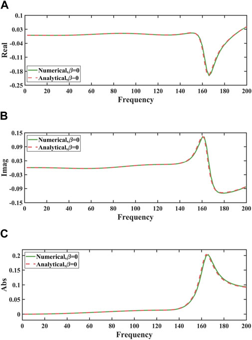
Figure 10. Sound pressure of the sphere model across various frequencies with $\beta =0$, incremented by a frequency step of 1 Hz. (A) β = 0, real part. (B) β = 0, imaginary part. (C) β = 0, sound pressure.

Figure 11 shows the sound pressure of the sphere model at different frequencies when $\beta =0$, $\beta =-1$, and $\beta =1$. From the figure, it can be seen that the sound pressure curves for $\beta =0$, $\beta =-1$, and $\beta =1$ are distinct, indicating that the impact of seabed reflection on the structural acoustic coupling system response in shallow water environments cannot be ignored. It is noteworthy that the sound pressure curves for $\beta =1$ and $\beta =-1$ are roughly distributed on either side of the sound pressure curve for $\beta =0$, and the two curves are essentially symmetric about the sound pressure curve for $\beta =0$. This phenomenon indicates that the effects of rigid and flexible seabeds on sound waves are opposite.

Figure 11

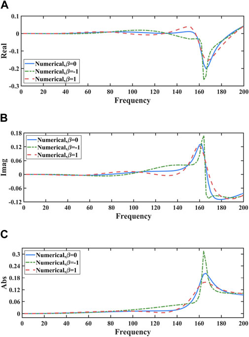
Figure 11. Sound pressure of the sphere model across various frequencies with $\beta =0$, $\beta =-1$, and $\beta =1$, incremented by a frequency step of 1 Hz. (A) Real part. (B) Imaginary part. (C) Sound pressure.

Figure 12 illustrates the sound pressure of the sphere model at various distances from the seabed, where $\tilde{r}$ denotes the distance from the model’s center to the seabed. It can be observed from the figure that when the frequency is less than 60Hz, the sound pressure curves for different $\tilde{r}$ are very close to each other; when the frequency exceeds 60Hz, the differences between the sound pressure curves for different $\tilde{r}$ gradually increase. This phenomenon confirms that the effect of ground reflection is frequency-dependent.

Figure 12

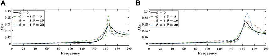
Figure 12. Sound pressure in terms of frequencies with different distances from the seabed for the sphere model. (A) β = −1. (B) β = 1.

4.2 Acoustic scattering by a fish model

This section analyzes the acoustic field scattering by a fish model under the action of incident plane waves, taking into account the reflection effects of the seabed, as shown in Figure 13. This subsection calculates the sound pressure and displacement under incident plane waves at different frequencies. The incident plane waves propagate along the positive x-axis with a unit amplitude and are scattered by the underwater model.

Using Catmull-Clark subdivision surfaces, two fish models with 54,216 and 222 mesh points were constructed. Figure 14 illustrates the sound pressure curves as a function of frequency for the fish models with 54,216 and 222 mesh points, respectively. The computation times for a single frequency were 483 s and 1,016 s for each model. As shown in the figure, the differences in the sound pressure curves between the two mesh densities are minor, with only slight fluctuations that are acceptable considering the significant disparity in computation times. Therefore, this study selects the fish model with 54,216 mesh points to optimize computational efficiency while maintaining acceptable accuracy.

When analyzing the acoustic scattering of the fish model, we found that the computation time for the traditional Catmull-Clark subdivision surfaces coupled with the FEM-BEM method was 5,143 s, whereas the computation time for the Catmull-Clark subdivision surfaces accelerated by FMM and coupled with the FEM-BEM method was only 483 s.

Figure 13

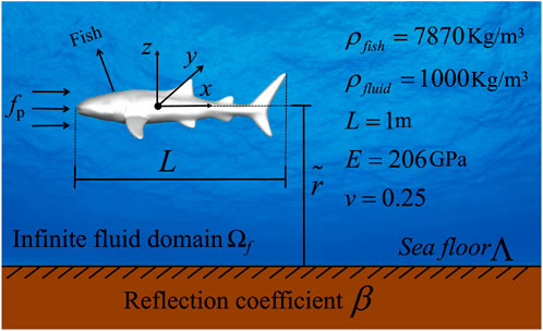
Figure 13. Acoustic-structural interaction system for the fish model.

Figure 14

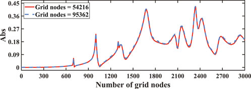
Figure 14. The numerical results of the fish model are verified in the convergence of two mesh node numbers.

Figure 15 shows the distribution of displacement and sound pressure for the fish model at a distance of 0.5 m from the seabed. As shown in the figure, the sound pressure and displacement distributions are symmetric along the x-axis. The magnitude order of the various displacement components of the fish model at different frequencies is not the same. For instance, at a frequency of 1,000 Hz, the displacement component in the x-direction is the largest, and the displacement component in the z-direction is the smallest; at a frequency of 3,000 Hz, the displacement component in the z-direction is the largest, and the displacement component in the y-direction is the smallest.

Figure 15

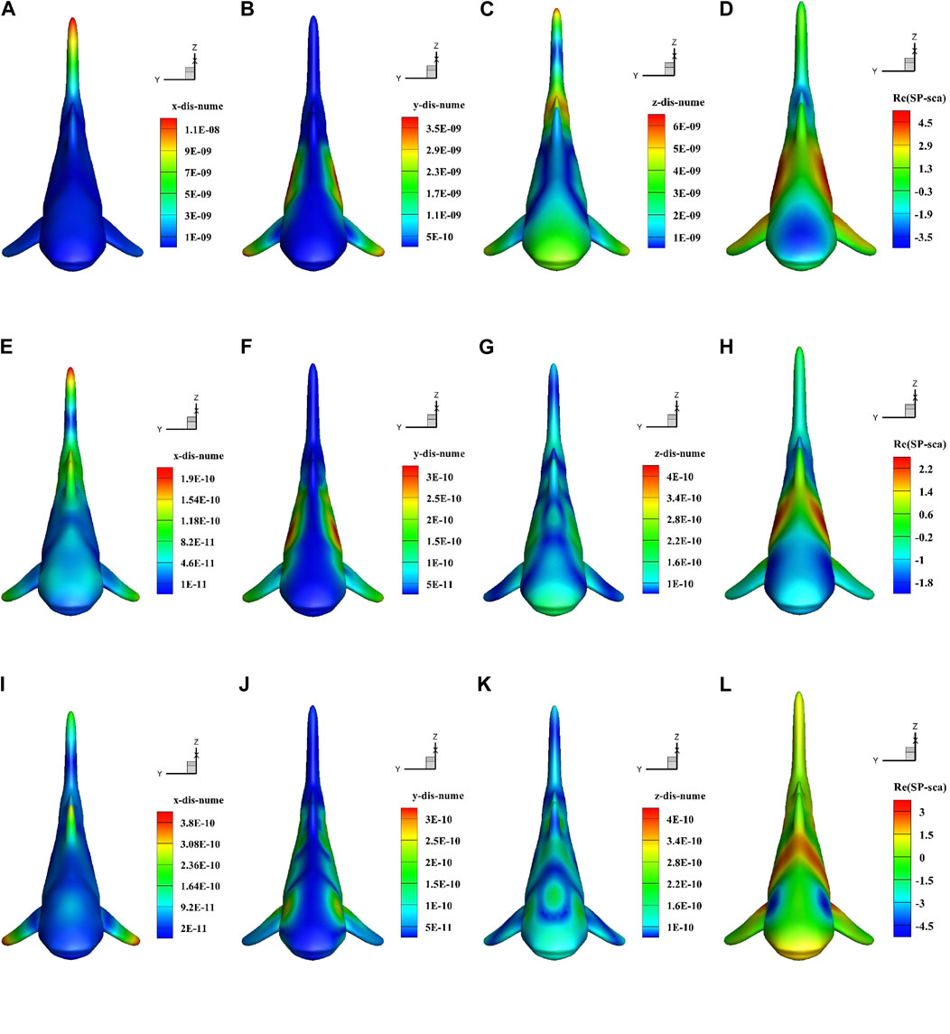
Figure 15. Sound pressure and displacement distributions on the surface of a fish model: the first three columns depict the three components of displacement, while the fourth column shows the sound pressure. (A) 1000 Hz, displacement x. (B) 1000 Hz, displacement y. (C) 1000 Hz, displacement z. (D) 1000 Hz,sound pressure. (E) 2000 Hz, displacement x. (F) 2000 Hz, displacement y. (G) 2000 Hz, displacement z. (H) 2000 Hz, sound pressure. (I) 3000 Hz, displacement x. (J) 3000 Hz, displacement y. (K) 3000 Hz, displacement z. (L) 3000 Hz, sound pressure.

Figure 16 displays the sound pressure of the fish model at different frequencies for $\beta =0$, $\beta =-1$, and $\beta =1$, with a frequency range of [03,000]Hz and a frequency step of 10 Hz. As shown in the figure, the sound pressure on the surface of the fish model varies with $\beta$. When the frequency is within the range of [0.600]Hz, the sound pressure curves for $\beta =0$, $\beta =-1$, and $\beta =1$ match very closely. However, when the frequency exceeds 600Hz, differences begin to emerge among them. This phenomenon once again confirms that the seabed reflection effect is frequency-dependent, not only for spherical models but also for complex models, and it also validates the necessity of considering the seabed reflection effect.

Figure 16

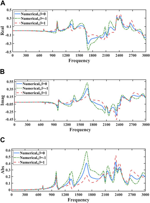
Figure 16. Sound pressure in terms of frequencies with different seabed reflection coefficient for the fish model: frequency steps of 10 Hz. (A) Real part. (B) Imaginary part. (C) Sound pressure.

Figure 17 illustrates the sound pressure of the fish model at various distances from the seabed. It can be observed from the figure that as the distance from the seabed increases, the sound pressure curve gradually aligns with the sound pressure curve for $\beta =0$. This phenomenon indicates that in shallow sea areas, the seabed reflection effect must be taken into account, while in deep sea areas, the seabed reflection effect can be selectively considered based on needs. This phenomenon is related to the nature of the seabed.

Figure 17

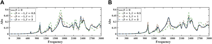
Figure 17. Sound pressure in terms of frequencies with different distances from the seabed for the fish model. (A) β = −1. (B) β = 1.

5 Conclusion

This paper presents a novel algorithm for analyzing the interaction between sound wave propagation and the vibration of underwater thin-shell structures, taking into account the effects of seabed reflection. We couple FEM with BEM to solve for shell vibrations and sound wave propagation in an infinite domain. To consider the effects of seabed reflection, the BEM employs a half-space fundamental solution approach. Within the isogeometric framework, geometric modeling is conducted using Catmull-Clark subdivision surfaces, and the same basis functions used for geometric modeling are applied to discretize the physical fields of the coupled FEM/BEM system. The use of isogeometric analysis maintains geometric accuracy, reduces meshing efforts, and produces high-order continuous fields, enabling the application of Kirchhoff-Love shell theory. Additionally, FMM is formulated to accelerate vibro-acoustic simulations. The precision of this algorithm is demonstrated through numerical examples.This study also has certain limitations. The current model’s assumption of linear elastic material properties, while suitable for small deformations and stresses, does not capture nonlinear behaviors under extreme conditions. The absence of fluid-structure interactions (FSI) in the present model may overlook critical phenomena such as damping and dynamic loading from fluid flows. Furthermore, the simplified treatment of seabed topographies with predefined reflection coefficients $\beta$ limits the model’s applicability to real-world scenarios.In the future, incorporating nonlinear material models, fluid-structure interaction modeling, and the uncertainty of seabed reflection coefficients into the model will ensure that the proposed algorithm not only maintains high computational efficiency but also delivers accurate and reliable results in complex vibration-acoustic analyses.

Data availability statement

The raw data supporting the conclusions of this article will be made available by the authors, without undue reservation.

Author contributions

XZ: Conceptualization, Formal Analysis, Methodology, Project administration, Resources, Software, Writing–original draft. KA: Conceptualization, Formal Analysis, Writing–original draft. SY: Data curation, Investigation, Resources, Software, Validation, Visualization, Writing–original draft. QP: Conceptualization, Formal Analysis, Funding acquisition, Resources, Software, Supervision, Writing–review and editing. GL: Data curation, Validation, Visualization, Writing–original draft.

Funding

The author(s) declare that financial support was received for the research, authorship, and/or publication of this article. Sponsored by the Henan Provincial Key R&D and Promotion Project under Grant No. 232102220033, the Zhumadian 2023 Major Science and Technology Special Project under Grant No. ZMDSZDZX2023002, and the Postgraduate Education Reform and Quality Improvement Project of Henan Province under Grant No. YJS2023JD52.

Conflict of interest

The authors declare that the research was conducted in the absence of any commercial or financial relationships that could be construed as a potential conflict of interest.

Generative AI statement

The author(s) declare that no Generative AI was used in the creation of this manuscript.

Publisher’s note

All claims expressed in this article are solely those of the authors and do not necessarily represent those of their affiliated organizations, or those of the publisher, the editors and the reviewers. Any product that may be evaluated in this article, or claim that may be made by its manufacturer, is not guaranteed or endorsed by the publisher.

References

1. Belibassakis K, Prospathopoulos J. A 3D-BEM for underwater propeller noise propagation in the ocean environment including hull scattering effects. Ocean Eng (2023) 286:115544. doi:10.1016/j.oceaneng.2023.115544

CrossRef Full Text | Google Scholar

2. Helal KM, Fragasso J, Moro L. Effectiveness of ocean gliders in monitoring ocean acoustics and anthropogenic noise from ships: a systematic review. Ocean Eng (2024) 295:116993. doi:10.1016/j.oceaneng.2024.116993

CrossRef Full Text | Google Scholar

3. Li Z, Zhang Y, Yang A. Numerical study on the flow-induced noise from waterjet-propelled ship regarding a flexible boundary. Ocean Eng (2023) 287:115911. doi:10.1016/j.oceaneng.2023.115911

CrossRef Full Text | Google Scholar

4. Viitanen V, Hynninen A, Sipilä T. Computational fluid dynamics and hydroacoustics analyses of underwater radiated noise of an ice breaker ship. Ocean Eng (2023) 279:114264. doi:10.1016/j.oceaneng.2023.114264

CrossRef Full Text | Google Scholar

5. Cheng Y, Du W, Dai S, Yuan Z, Incecik A. Wave energy conversion by an array of oscillating water columns deployed along a long-flexible floating breakwater. Renew Sustainable Energy Rev (2024) 192:114206. doi:10.1016/j.rser.2023.114206

CrossRef Full Text | Google Scholar

6. Jiao J, Huang S, Tezdogan T, Terziev M, Soares CG. Slamming and green water loads on a ship sailing in regular waves predicted by a coupled cfd–fea approach. Ocean Eng (2021) 241:110107. doi:10.1016/j.oceaneng.2021.110107

CrossRef Full Text | Google Scholar

7. Shao X, Yao HD, Ringsberg JW, Li Z, Johnson E. Performance analysis of two generations of heaving point absorber wecs in farms of hexagon-shaped array layouts. Ships and Offshore Structures (2024) 19:687–98. doi:10.1080/17445302.2024.2317658

CrossRef Full Text | Google Scholar

8. Shen XW, Du CB, Jiang SY, Zhang P, Chen LL. Multivariate uncertainty analysis of fracture problems through model order reduction accelerated sbfem. Appl Math Model (2024) 125:218–40. doi:10.1016/j.apm.2023.08.040

CrossRef Full Text | Google Scholar

9. Li Z, Bouscasse B, Ducrozet G, Gentaz L, Le Touzé D, Ferrant P. Spectral wave explicit Navier-Stokes equations for wave-structure interactions using two-phase computational fluid dynamics solvers. Ocean Eng (2021) 221:108513. doi:10.1016/j.oceaneng.2020.108513

CrossRef Full Text | Google Scholar

10. Gao Z, Li Z, Liu Y. A time-domain boundary element method using a kernel-function library for 3d acoustic problems. Eng Anal Boundary Elem (2024) 161:103–12. doi:10.1016/j.enganabound.2024.01.001

CrossRef Full Text | Google Scholar

11. Chen L, Huo R, Lian H, Yu B, Zhang M, Natarajan S, et al. Uncertainty quantification of 3d acoustic shape sensitivities with generalized nth-order perturbation boundary element methods. Computer Methods Appl Mech Eng (2025) 433:117464. doi:10.1016/j.cma.2024.117464

CrossRef Full Text | Google Scholar

12. Chen L, Lian H, Liu Z, Chen H, Atroshchenko E, Bordas S. Structural shape optimization of three dimensional acoustic problems with isogeometric boundary element methods. Computer Methods Appl Mech Eng (2019) 355:926–51. doi:10.1016/j.cma.2019.06.012

CrossRef Full Text | Google Scholar

13. Ren Y, Qin Y, Pang F, Wang H, Su Y, Li H. Investigation on the flow-induced structure noise of a submerged cone-cylinder-hemisphere combined shell. Ocean Eng (2023) 270:113657. doi:10.1016/j.oceaneng.2023.113657

CrossRef Full Text | Google Scholar

14. Kha J, Karimi M, Maxit L, Skvortsov A, Kirby R. Forced vibroacoustic response of a cylindrical shell in an underwater acoustic waveguide. Ocean Eng (2023) 273:113899. doi:10.1016/j.oceaneng.2023.113899

CrossRef Full Text | Google Scholar

15. Huang H, Zou MS, Jiang LW. Study on the integrated calculation method of fluid–structure interaction vibration, acoustic radiation, and propagation from an elastic spherical shell in ocean acoustic environments. Ocean Eng (2019) 177:29–39. doi:10.1016/j.oceaneng.2019.02.032

CrossRef Full Text | Google Scholar

16. Chen LL, Lian HJ, Dong HW, Yu P, Jiang SJ, Bordas SPA. Broadband topology optimization of three-dimensional structural-acoustic interaction with reduced order isogeometric FEM/BEM. J Comput Phys (2024) 509:113051. doi:10.1016/j.jcp.2024.113051

CrossRef Full Text | Google Scholar

17. Chen L, Lian H, Pei Q, Meng Z, Jiang S, Dong H, et al. Fem-bem analysis of acoustic interaction with submerged thin-shell structures under seabed reflection conditions. Ocean Eng (2024) 309:118554. doi:10.1016/j.oceaneng.2024.118554

CrossRef Full Text | Google Scholar

18. Choi YM, Bouscasse B, Ducrozet G, Seng S, Ferrant P, Kim ES, et al. An efficient methodology for the simulation of nonlinear irregular waves in computational fluid dynamics solvers based on the high order spectral method with an application with openfoam. Int J Naval Architecture Ocean Eng (2023) 15:100510. doi:10.1016/j.ijnaoe.2022.100510

CrossRef Full Text | Google Scholar

19. Wei Y, Incecik A, Tezdogan T. A hydroelasticity analysis of a damaged ship based on a two-way coupled CFD-DMB method. Ocean Eng (2023) 274:114075. doi:10.1016/j.oceaneng.2023.114075

CrossRef Full Text | Google Scholar

20. Liu D, Havranek Z, Marburg S, Peters H, Kessissoglou N. Non-negative intensity and back-calculated non-negative intensity for analysis of directional structure-borne sound. The J Acoust Soc America (2017) 142:117–23. doi:10.1121/1.4990374

PubMed Abstract | CrossRef Full Text | Google Scholar

21. Wilkes DR, Peters H, Croaker P, Marburg S, Duncan AJ, Kessissoglou N. Non-negative intensity for coupled fluid-structure interaction problems using the fast multipole method. The J Acoust Soc America (2017) 141:4278–88. doi:10.1121/1.4983686

PubMed Abstract | CrossRef Full Text | Google Scholar

22. Faugeras B, Heumann H. FEM-BEM coupling methods for tokamak plasma axisymmetric free-boundary equilibrium computations in unbounded domains. The J Acoust Soc America (2017) 343:201–16. doi:10.1016/j.jcp.2017.04.047

CrossRef Full Text | Google Scholar

23. Everstine GC, Henderson FM. Coupled finite element/boundary element approach for fluid-structure interaction. The J Acoust Soc America (1990) 87:1938–47. doi:10.1121/1.399320

CrossRef Full Text | Google Scholar

24. Chen LL, Lian HJ, Liu ZW, Gong Y, Zheng CJ, Bordas SPA. Bi-material topology optimization for fully coupled structural-acoustic systems with isogeometric FEM–BEM. Eng Anal Boundary Elem (2022) 135:182–95. doi:10.1016/j.enganabound.2021.11.005

CrossRef Full Text | Google Scholar

25. Xu J, Wang L, Yuan J, Luo Z, Wang Z, Zhang B, et al. Dlfsi: a deep learning static fluid-structure interaction model for hydrodynamic-structural optimization of composite tidal turbine blade. Renew Energy (2024) 224:120179. doi:10.1016/j.renene.2024.120179

CrossRef Full Text | Google Scholar

26. Chen LL, Cheng RH, Li SZ, Lian HJ, Zheng CJ, Bordas SPA. A sample-efficient deep learning method for multivariate uncertainty qualification of acoustic-vibration interaction problems. Computer Methods Appl Mech Eng (2022) 393:114784. doi:10.1016/j.cma.2022.114784

CrossRef Full Text | Google Scholar

27. Zou MS, Wu YS, Liu SX. A three-dimensional sono-elastic method of ships in finite depth water with experimental validation. Ocean Eng (2018) 164:238–47. doi:10.1016/j.oceaneng.2018.06.052

CrossRef Full Text | Google Scholar

28. Jiang LW, Zou MS, Liu SX, Huang H. Calculation method of acoustic radiation for floating bodies in shallow sea considering complex ocean acoustic environments. J Sound Vibration (2020) 476:115330. doi:10.1016/j.jsv.2020.115330

CrossRef Full Text | Google Scholar

29. Qi LB, Yu Y, Tang HC, Zou MS. Study of the influence of added water and contained water on structural vibrations and acoustic radiation using different dynamic modeling methods. J Hydrodynamics (2023) 35:1157–67. doi:10.1007/s42241-024-0087-6

CrossRef Full Text | Google Scholar

30. Huang H, Zou MS, Jiang LW. Study on the integrated calculation method of fluid-structure interaction vibration, acoustic radiation, and propagation from an elastic spherical shell in ocean acoustic environments. Ocean Eng (2019) 177:29–39. doi:10.1016/j.oceaneng.2019.02.032

CrossRef Full Text | Google Scholar

31. Liu XL, Wu HJ, Sun RH, Jiang WK. A fast multipole boundary element method for half-space acoustic problems in a subsonic uniform flow. Eng Anal Boundary Elem (2022) 137:16–28. doi:10.1016/j.enganabound.2022.01.008

CrossRef Full Text | Google Scholar

32. Messaoudi A, Cottereau R, Gomez C. Boundary effects in radiative transfer of acoustic waves in a randomly fluctuating half-space. Multiscale Model and Simulation (2023) 21:1299–321. doi:10.1137/22m1537795

CrossRef Full Text | Google Scholar

33. Yasuda Y, Higuchi K, Oshima T, Sakuma T. An efficient technique for plane-symmetrical acoustic problems in low-frequency FMBEM. INTER-NOISE NOISE-CON Congress Conf Proc (Institute Noise Control Engineering) (2011) 593–601.

Google Scholar

34. Yasuda Y, Sakuma T. A technique for plane-symmetric sound field analysis in the fast multipole boundary element method. J Comput Acoust (2005) 13:71–85. doi:10.1142/s0218396x05002591

CrossRef Full Text | Google Scholar

35. Brunner D, Of G, Junge M, Steinbach O, Gaul L. A fast BE-FE coupling scheme for partly immersed bodies. Int J Numer Methods Eng (2010) 81:28–47. doi:10.1002/nme.2672

CrossRef Full Text | Google Scholar

36. Magisano D, Corrado A, Leonetti L, Kiendl J, Garcea G. Large deformation Kirchhoff–Love shell hierarchically enriched with warping: isogeometric formulation and modeling of alternating stiff/soft layups. Computer Methods Appl Mech Eng (2024) 418:116556. doi:10.1016/j.cma.2023.116556

CrossRef Full Text | Google Scholar

37. Zhang R, Zhao G, Wang W, Du X. Large deformation frictional contact formulations for isogeometric Kirchhoff–Love shell. Int J Mech Sci (2023) 249:108253. doi:10.1016/j.ijmecsci.2023.108253

CrossRef Full Text | Google Scholar

38. Duan J, Zhang L, Sun X, Chen W, Da L. An equivalent source CVIS method and its application in predicting structural vibration and acoustic radiation in ocean acoustic channe. Ocean Eng (2021) 222:108570. doi:10.1016/j.oceaneng.2021.108570

CrossRef Full Text | Google Scholar

39. Chen LL, Lian HJ, Natarajan S, Zhao W, Chen XY, Bordas SPA. Multi-frequency acoustic topology optimization of sound-absorption materials with isogeometric boundary element methods accelerated by frequency-decoupling and model order reduction techniques. Computer Methods Appl Mech Eng (2022) 395:114997. doi:10.1016/j.cma.2022.114997

CrossRef Full Text | Google Scholar

40. Xie K, Chen M, Zhang L, Li W, Dong W. A unified semi-analytic method for vibro-acoustic analysis of submerged shells of revolution. Ocean Eng (2019) 189:106345. doi:10.1016/j.oceaneng.2019.106345

CrossRef Full Text | Google Scholar

41. Li R, Liu Y, Ye W. A fast direct boundary element method for 3d acoustic problems based on hierarchical matrices. Eng Anal Boundary Elem (2023) 147:171–80. doi:10.1016/j.enganabound.2022.11.035

CrossRef Full Text | Google Scholar

42. Hughes TJR, Cottrell JA, Bazilevs Y. Isogeometric analysis: CAD, finite elements, NURBS, exact geometry and mesh refinement. Computer Methods Appl Mech Eng (2005) 194:4135–95. doi:10.1016/j.cma.2004.10.008

CrossRef Full Text | Google Scholar

43. Chen LL, Wang ZW, Lian HJ, Ma YJ, Meng ZX, Li P, et al. Reduced order isogeometric boundary element methods for CAD-integrated shape optimization in electromagnetic scattering. Computer Methods Appl Mech Eng (2024) 419:116654. doi:10.1016/j.cma.2023.116654

CrossRef Full Text | Google Scholar

44. Yang HS, Dong CY, Wu YH. Non-conforming interface coupling and symmetric iterative solution in isogeometric fe-be analysis. Computer Methods Appl Mech Eng (2021) 373:113561. doi:10.1016/j.cma.2020.113561

CrossRef Full Text | Google Scholar

45. Qu YL, Zhou ZB, Chen LL, Lian HJ, Li XD, Hu ZM, et al. Uncertainty quantification of vibro-acoustic coupling problems for robotic manta ray models based on deep learning. Ocean Eng (2024) 299:117388. doi:10.1016/j.oceaneng.2024.117388

CrossRef Full Text | Google Scholar

46. Chen L, Liu L, Zhao W, Liu C. An isogeometric approach of two dimensional acoustic design sensitivity analysis and topology optimization analysis for absorbing material distribution. Computer Methods Appl Mech Eng (2018) 336:507–32. doi:10.1016/j.cma.2018.03.025

CrossRef Full Text | Google Scholar

47. Zhang S, Li T, Zhu X, Yin C, Li Q. Far field acoustic radiation and vibration analysis of combined shells submerged at finite depth from free surface. Ocean Eng (2022) 252:111198. doi:10.1016/j.oceaneng.2022.111198

CrossRef Full Text | Google Scholar

48. Chen LL, Lian HJ, Xu YM, Li SZ, Liu ZW, Atroshchenko E, et al. Generalized isogeometric boundary element method for uncertainty analysis of time-harmonic wave propagation in infinite domains. Appl Math Model (2023) 114:360–78. doi:10.1016/j.apm.2022.09.030

CrossRef Full Text | Google Scholar

49. Wu YH, Dong CY, Yang HS, Sun FL. Isogeometric symmetric FE-BE coupling method for acoustic-structural interaction. Appl Mathematics Comput (2021) 393:125758. doi:10.1016/j.amc.2020.125758

CrossRef Full Text | Google Scholar

50. Liu ZW, Bian PL, Qu YL, Huang WC, Chen LL, Chen JB A galerkin approach for analysing coupling effects in the piezoelectric semiconducting beams. Eur J Mechanics-A/Solids (2024) 103:105145. doi:10.1016/j.euromechsol.2023.105145

CrossRef Full Text | Google Scholar

51. Cao G, Yu B, Chen L, Yao W. Isogeometric dual reciprocity BEM for solving non-fourier transient heat transfer problems in FGMs with uncertainty analysis. Int J Heat Mass Transfer (2023) 203:123783. doi:10.1016/j.ijheatmasstransfer.2022.123783

CrossRef Full Text | Google Scholar

52. Zhang S, Yu B, Chen L. Non-iterative reconstruction of time-domain sound pressure and rapid prediction of large-scale sound field based on IG-DRBEM and POD-RBF. J Sound Vibration (2024) 573:118226. doi:10.1016/j.jsv.2023.118226

CrossRef Full Text | Google Scholar

53. Catmull E, Clark J. Recursively generated B-spline surfaces on arbitrary topological meshes. Computer-Aided Des (1978) 10:350–5. doi:10.1016/0010-4485(78)90110-0

CrossRef Full Text | Google Scholar

54. Wu S, Xiang Y, Liu B, Li G. A weak-form interpolation meshfree method for computing underwater acoustic radiation. Ocean Eng (2021) 233:109105. doi:10.1016/j.oceaneng.2021.109105

CrossRef Full Text | Google Scholar

55. Kirkup SM. The boundary element method in acoustics (Integrated sound software) (2007).

Google Scholar

56. Wu TW, Ochmann M. Boundary element acoustics fundamentals and computer codes. The J Acoust Soc America (2002) 111:1507–8. doi:10.1121/1.1456929

CrossRef Full Text | Google Scholar

57. Chen L, Lu C, Lian H, Liu Z, Zhao W, Li S, et al. Acoustic topology optimization of sound absorbing materials directly from subdivision surfaces with isogeometric boundary element methods. Computer Methods Appl Mech Eng (2020) 362:112806. doi:10.1016/j.cma.2019.112806

CrossRef Full Text | Google Scholar

58. Gao XW, Yang K, Wang J. An adaptive element subdivision technique for evaluation of various 2D singular boundary integrals. Eng Anal Boundary Elem (2008) 32:692–6. doi:10.1016/j.enganabound.2007.12.004

CrossRef Full Text | Google Scholar

59. Chen J, Hong H. Review of dual boundary element methods with emphasis on hypersingular integrals and divergent series. Appl Mech Rev (1999) 52:17–33. doi:10.1115/1.3098922

CrossRef Full Text | Google Scholar

60. Zhong Y, Zhang J, Dong Y, Yuan L, Lin W, Tang J. A serendipity triangular patch for evaluating weakly singular boundary integrals. Eng Anal Boundary Elem (2016) 69:86–92. doi:10.1016/j.enganabound.2016.05.003

CrossRef Full Text | Google Scholar

61. Zhang J, Qin X, Xu H, Li G. A boundary face method for potential problems in three dimensions. Int J Numer Methods Eng (2009) 80:320–37. doi:10.1002/nme.2633

CrossRef Full Text | Google Scholar

62. Rong J, Wen L, Xiao J. Efficiency improvement of the polar coordinate transformation for evaluating BEM singular integrals on curved elements. Eng Anal Boundary Elem (2014) 38:83–93. doi:10.1016/j.enganabound.2013.10.014

CrossRef Full Text | Google Scholar

63. Greengard L, Rokhlin V. A fast algorithm for particle simulations. J Comput Phys (1987) 73:325–48. doi:10.1016/0021-9991(87)90140-9

CrossRef Full Text | Google Scholar

64. Chen LL, Zhao J, Lian HJ, Yu B, Atroshchenko E, Li P. A BEM broadband topology optimization strategy based on taylor expansion and soar method-application to 2d acoustic scattering problems. Int J Numer Methods Eng (2023) 124:5151–82. doi:10.1002/nme.7345

CrossRef Full Text | Google Scholar