Damage spreading and coupling in spin glasses and hard spheres

We study the connection between damage spreading, a phenomenon long discussed in the physics literature, and the coupling of Markov chains, a technique used to bound the mixing time. We discuss in parallel the Edwards–Anderson spin-glass model and the hard-disk system, focusing on how coupling provides bounds on the extension of the paramagnetic and liquid phases. We also work out the connection between path coupling and damage spreading. Numerically, the scaling analysis of the mean coupling time determines a critical point between fast and slow couplings. The exact relationship between fast coupling and disordered phases has not been established rigorously, but we suggest that it will ultimately enhance our understanding of phase behavior in disordered systems.

1 Introduction

Monte Carlo simulations based on Markov chains [36, 37] play an important role in the study of complex systems in physics and other sciences. In a given sample space, Markov chains perform random walks that, in their large-time steady state, visit configurations according to a prescribed stationary distribution (often the Boltzmann distribution). At early times, in contrast, after its start from a given initial configuration, each Markov chain samples different time-dependent distributions. The characterization of convergence (that is, of the mixing timescale [39] for approaching the stationary distribution) is of greatest importance as, by definition, convergence is required for sampling from the prescribed distribution and for estimating mean values of observables (pressure, specific heat, and internal energy) as running averages. Moreover, the mixing timescale by itself carries important information on the sampling problem. In a physics context, the sudden slowdown of mixing and relaxation times (without reference to any observable) often indicates a phase transition. Well-known examples are the slowdown of the Glauber dynamics at the paramagnetic–ferromagnetic transition in the Ising model [22, 41], as well as the glass transition, which is defined through the slowdown of relaxation processes (although it is not of thermodynamic origin). The spin-glass transition is believed to be signaled by a stark increase in the relaxation times at low temperatures [23]. In addition, in certain local Monte Carlo algorithms for particle systems, fast mixing (in a way that we will discuss later) is only possible in the liquid phase [32], so a statement about thermodynamic phases is obtained from an analysis of mixing times without invoking observables. However, establishing mixing and relaxation times can be an arduous task, both in practice and in theory.

As convergence sets in, samples and empirical mean values (running averages) become independent of initial configurations. Much stronger than mere independence, samples can actually become identical for two (or more) different initial configurations. This phenomenon, called coupling, is a focus of the present article. A coupling is a bivariate stochastic process that starts from two far-away initial configurations at time $t=0$, say, $x_0$ and $y_0$, under the condition that the projected evolution of $x_t$ and of $y_t$, taken separately, realize a Markov chain with its transition matrix $P$. When the evolutions of the two trajectories meet at the coupling time ${\tau }_{\text{coup}}$, with $x_{{\tau }_{\text{coup}}}=y_{{\tau }_{\text{coup}}}$, they are glued together for all later times (see the lhs of Figure 1). Couplings of a given Markov chain can take many different forms, but for all of them, the coupling time provides an upper bound for the mixing time. This property has been used for almost a century to prove theorems on Markov chains [20], as cited in Ref. [28]. Among many other developments, a more recent version of coupling, known as “coupling from the past” [48], has allowed for the perfect sampling of the stationary distribution without any error, completely sidestepping the estimation of mixing-time scales.

Figure 1

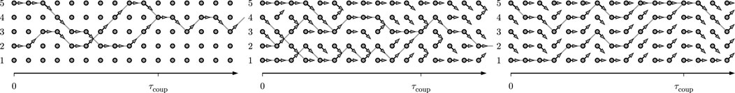
Figure 1. Coupling for the random walk on a path graph (arrows point into the three directions with equal probabilities, and those leaving the graph are replaced by straight arrows). Left: Classic coupling: the two random walks advance independently until they merge at ${\tau }_{\text{coup}}$. Middle: A random-map implementation of the classic coupling (independent arrows). Right: A random-share, monotone coupling, where at a given time, all configurations are updated with the same random number. Trajectories cannot cross.

The path-coupling approach [13] attempts to bound the global coupling time through an analysis that is local in both time and space. The two far-away initial configurations are imagined as end points of a “path” of many configurations. Configurations that are connected on the path are neighbors in the sample space with respect to a given metric. For the one-dimensional random walk, the metric may correspond to the Euclidean distance (see the lhs of Figure 1). For Ising systems, the metric could be the Hamming distance: neighboring configurations differ by only one spin. Similarly, for low-density systems of $N$ hard spheres, neighboring configurations differ in only one sphere, which can be arbitrarily far away in the two configurations, while the other $N-1$ spheres coincide. It is often possible to deduce upper limits for the coupling time from the contraction rates for the individual path links. Path coupling was foreshadowed in the physics literature in a phenomenon termed “damage spreading” [53], which also studied such neighboring configurations under coupled-Markov-chain dynamics, a special type of coupling for Glauber dynamics. In the Ising model, for the same dynamics, the damage was found to disappear rapidly throughout the paramagnetic phase, a phenomenon later understood through the concept of “monotone coupling.” In the Ising spin-glass model, the damage was found to disappear above a finite temperature in the paramagnetic phase, even in two spatial dimensions, where the spin-glass transition temperature is believed to vanish. Attempts to directly connect the damage spreading with a thermodynamics process, such as a percolation transition, were finally unsuccessful. In other words, the connection between damage spreading, path coupling, and thermodynamics is that “fast” path coupling implies fast coupling, which implies fast mixing. Fast mixing, in turn, very often implies, in a physics context, that the thermodynamic phase is trivial. This can lead to non-trivial rigorous bounds on the extension of the paramagnetic phase for spin models [22] or the liquid phase for particle systems [32].

This article presents a unified description of coupling and damage spreading, using spin-glass and hard-sphere models as examples. In Section 2, we provide common definitions, discuss theoretical foundations, and explore the connection between coupling and mixing, as well as the relationship between the aforementioned path coupling and damage spreading. We also introduce the scaling approach to phase transitions that we later apply to the coupling phenomenon. Section 3 is dedicated to spin glasses. We discuss rigorous results and the generally accepted theoretical framework for the spin-glass model introduced by Edwards and Anderson. Additionally, we explore path coupling and damage spreading for this model. We further apply the scaling analysis to its mean coupling time, which suggests a phase transition between fast and slow couplings. Section 4 addresses the hard-sphere model, for which we can generally transpose all the theoretical approaches of Section 3. The conclusions of our work are presented in Section 5.

2 Theoretical foundations

In this section, we discuss some fundamentals of Markov chains and first concentrate on the connection between the convergence of a Markov chain expressed through its mixing time and any of its couplings (Section 2.1). The special case of “monotone” coupling, which we also address, has important consequences for the ferromagnetic Ising model, although it does not apply to spin-glass models or to hard spheres in more than one dimension [49]. We then discuss damage spreading in terms of path coupling (Section 2.2). We will discuss the intimate relationship between a global view on coupling and a purely local view, which only surveys configurations that differ minimally. We finally discuss in Section 2.3 the scaling approach to coupling that later will be shown to apply both to spin glasses and to hard spheres.

2.1 Mixing, coupling, and monotone coupling

We consider a Markov chain with samples $x_t$ at time $t=\mathrm{0,1},\dots$ in a sample space $\mathrm{\Omega }$. In our case, its transition matrix $P$ implements the heat-bath algorithm [17, 26, 27] (in other words, Glauber dynamics) for the Edwards–Anderson model or a version of the Metropolis algorithm [43] for hard spheres. We define the element $P(x,x^{\prime })$ as the conditional probability to move from configuration $x$ at time $t$ to configuration $x^{\prime }$ at time $t+1$. With an initial configuration $x_0$, the distribution ${\pi }^{\{t=0\}}$ is a delta function centered at $x_0$. The distribution evolves over time as ${\pi }^{\{t+1\}}(x^{\prime })={\sum }_x{\pi }^{\{t\}}(x)P(x,x^{\prime })$ for each time step $t$. The approach to equilibrium is quantified by the mixing time, which is the time it takes for ${\pi }^{\{t\}}$ (which depends on the choice of $x_0$) to approach the stationary distribution ${\pi }^{\{t\to \infty \}}=\pi$:

${\tau }_{\text{mix}}\left(ϵ\right)=\underset{t}{\min }\left\{\underset{d\left(t\right)}{\underbrace{\underset{x_0\in \mathrm{\Omega }}{\max }{‖{\pi }^{\{t\}}-\pi ‖}_{\text{TV}}}}<ϵ\right\}.(1)$

Here, $\Vert \cdots {\Vert }_{\text{TV}}$ denotes the total variation distance [39], that is, one half of the absolute difference between ${\pi }^{\{t\}}$ and $\pi$ over all the sample space, and $ϵ$ is an arbitrary positive parameter that must be taken smaller than $\frac{1}{2}$. In Equation 1, the “$\max$” refers to the worst initial choice for the approach of ${\pi }^{\{t\}}$ (which depends on $x_0$) to $\pi$, and this allows one to define the distance $d(t)$ between ${\pi }^{\{t\}}$ and $\pi$, without explicit reference to the starting distribution ${\pi }^{\{t=0\}}$. The mixing time is a non-asymptotic time scale [2] that describes the initial approach of ${\pi }^{\{t\}}$ toward the equilibrium distribution $\pi$ on a finite distance scale $ϵ$. It comes with an exponential bound, valid from ${\tau }_{\text{mix}}$ up to $t\to \infty$, while the asymptotic approach toward equilibrium, described by the (absolute) inverse gap of the transition matrix, can be much faster [39].

For a given transition matrix $P$ of a Markov chain on a sample space $\mathrm{\Omega }$, a coupling is defined as a bivariate stochastic process with a configuration $(x_t,y_t)$ at time $t$ on the sample space $\mathrm{\Omega }\times \mathrm{\Omega }$, such that

$\mathbb{P}\left[x_{t+1}=x^{\prime }|\left(x_t,y_t\right)=\left(x,y\right)\right]=P\left(x,x^{\prime }\right),$

$\mathbb{P}\left[y_{t+1}=y^{\prime }|\left(x_t,y_t\right)=\left(x,y\right)\right]=P\left(y,y^{\prime }\right).$

The bivariate process that updates the two copies $x$ and $y$ need not be Markovian [28] at a difference of its two projections. Non-Markovian couplings are theoretically important but have not been used yet in applications. Markovian couplings are described by a transition matrix $P^{\text{coup}}[(\cdot ),(\cdot )]$ on the sample space $\mathrm{\Omega }\times \mathrm{\Omega }$ that satisfies

${\displaystyle \sum _{y^{\prime }}}{P}^{\text{coup}}[(x,y),(x^{\prime },y^{\prime })]=P\left(x,x^{\prime }\right),$

${\displaystyle \sum _{x^{\prime }}}{P}^{\text{coup}}[(x,y),(x^{\prime },y^{\prime })]=P\left(y,y^{\prime }\right),$

so that the transition matrix of the coupled Markov chain, which acts on two copies of the sample space $\mathrm{\Omega }$, when projected on either copy, returns the original transition matrix.

Couplings can take a variety of forms. The “classic” coupling performs two statistically independent Markov chains until, by accident, they couple, from when on they are glued together:

$P^{\text{coup}}[(x,y),(x^{\prime },y^{\prime })]=\left\{\begin{array}{cc}P\left(x,x^{\prime }\right)P\left(y,y^{\prime }\right)\hfill & \text{if\hspace{0.17em}}x\ne y,\hfill \\ P\left(x,x^{\prime }\right)\hfill & \text{if\hspace{0.17em}}x=y,x^{\prime }=y^{\prime },\hfill \\ 0\hfill & \text{if\hspace{0.17em}}x=y,x^{\prime }\ne y^{\prime },\hfill \end{array}\right.(2)$

(see the lhs of Figure 1). At the coupling time ${\tau }_{\text{coup}}$, the trajectories first meet:

${\tau }_{\text{coup}}=\underset{t}{\min }\left\{x_t=y_t\right\}.$

Transition matrices, as the ones in Equation 2, are implemented in Monte Carlo algorithms with the use of random elements, that is, one or several random numbers for selecting a particle or a spin, for choosing a move, and for accepting or rejecting it, etc. For example, the move from $x$ at time $t$ may produce an outcome $x^{\prime }$ that depends on the realization of the random element, but when this element is specified, as ${\mathrm{\Upsilon }}_t(x)$, it becomes a function called a random map $\{t\}\times \mathrm{\Omega }\to \mathrm{\Omega }:x\to x^{\prime }=\varphi \left[x,{\mathrm{\Upsilon }}_t(x)\right]$. The random map $\varphi \left[x,{\mathrm{\Upsilon }}_t(x)\right]$ implementing this move must satisfy

$\mathbb{P}\left\{\varphi \left[x,{\mathrm{\Upsilon }}_t\left(x\right)\right]=x^{\prime }\right\}=P\left(x,x^{\prime }\right),$

as it must reproduce the transition matrix $P$. A random map $\varphi$ (also called a “grand” coupling [39]) specifies a coupling, and it automatically implements a “gluing” operation, as two Markov chains that meet at a position $x$ at time $t$ encounter the same random element. For the classic coupling of Equation 2, the randomness at time $t$ is a vector ${\mathbf{\Upsilon }}_t=\{{\mathrm{\Upsilon }}_t(x):x\in \mathrm{\Omega }\}$ of i.i.d random variables, that is of random numbers drawn from the same distribution (see center of Figure 1). For the “random-share” coupling, one uses, at time $t$, the same random element for all configurations $x\in \mathrm{\Omega }$: ${\mathbf{\Upsilon }}_t=\{{\mathrm{\Upsilon }}_t,\dots ,{\mathrm{\Upsilon }}_t\}$. In other words, all configurations are updated with the same random numbers. Many other couplings exist, and it is only important that the projection onto a single copy produces a valid Markov chain. While every random map corresponds to a coupling, it appears that not all couplings (for example, the path couplings in Ref. [32]) can be expressed as random maps.

The connection between mixing times and coupling times is as follows ([39], corollary 5.3):

$d\left(t\right)\le \underset{x_0,y_0\in \mathrm{\Omega }}{\max }{\mathbb{P}}_{x_0,y_0}\left\{{\tau }_{\text{coup}}>t\right\},(3)$

where $d(t)$ is the distance entering the definition of the mixing time in Equation 1. From our previous discussion, it is evident that for random walks on large graphs, the classic coupling time can be much larger than the mixing time simply because the two Markov chains must hit the same configuration at the same time. In contrast, the random-share coupling time is of the same order as the mixing time for many random walks. In the problems at the focus of this article, we will witness different regimes, as a function of external parameters, that are separated by a phase transition. In this context, it is of great interest that an optimal coupling [28] realizes the coupling at time $t$ and at position $x_t$ of two Markov chains that have started at time $t=0$ at configurations $x_0$ and $y_0$ with the minimum of the probabilities to go from $x_0$ or from $y_0$ to $x_t$. The optimal coupling is non-Markovian and virtually impossible to construct in practice, but it demonstrates that the bound of Equation 3 can be saturated.

A special class of couplings for which the inequality of Equation 3 can be tight (up to logarithms) requires the concept of monotonicity. In monotone couplings, there exists a partial ordering “$⪯$” of configurations so that $x_t⪯y_t$ implies $x_{t+1}⪯y_{t+1}$. In terms of the random map, $x⪯y$ implies $\varphi (x,\mathbf{\Upsilon })⪯\varphi (y,\mathbf{\Upsilon })$. No partial ordering exists for the random walk on the path graph with a classic coupling, and trajectories of Markov chains may cross (see the lhs of Figure 1). In contrast, for the random-share coupling of the one-dimensional random walk (which is a grand coupling), the ordering is complete. For a monotone grand coupling, with $l$ the length of the longest “chain” in the partially ordered subset, the mean coupling time ${\tau }_{\text{coup}}$ satisfies

$⟨{\tau }_{\text{coup}}⟩<2{\tau }_{\text{mix}}\left(1/e\right)\left(1+\text{log}l\right).(4)$

With Equation 3, there are thus upper and lower bounds for the monotone coupling time in terms of the mixing time, and the two agree up to a logarithm. For a monotone coupling with extremal elements, one must only survey their evolution, which will bracket all other configurations (see the rhs of Figure 1). Full surveys are possible in other cases [15], but the upper bound in Equation 4 is then often lost.

2.2 Path coupling and damage spreading

We can consider families of Markov chains that correspond to physical systems with size $N$, which may represent the number of sites, spins, or particles. As $N$ increases and approaches infinity, under suitable conditions, such as constant temperature for spin systems or constant density for particle systems, the behavior of these systems can be studied. We may refer to “fast” coupling if the mean coupling time $⟨{\tau }_{\text{coup}}⟩$ scales not slower than a power of the system size $N$ (in later sections, we will use an $N\text{log}N$ scaling).

As mentioned in the introduction, we may imagine the worst-case initial configurations $x_0$ and $y_0$ as the end points of a path of configurations, with adjacent elements on the path being neighbors, with respect to some metric. Under some conditions, it is often possible to show that any pair of neighboring configurations come in expectation even closer after one step of the Markov chain, and this establishes that the distance between $x_1$ and $y_1$ contracts, and similarly for later times, leading to a proof of fast coupling [13].

The path-coupling analysis that is local in sample space and in time yet valid uniformly for any pair of neighboring configurations yields a rigorous global fast-coupling bound. We will discuss the limiting temperature $T_{\text{path}}$ for spin glasses and limiting density ${\eta }_{\text{path}}$ for hard-sphere systems for which the uniform contraction allows one to prove fast coupling. However, the path-coupling approach is quite conservative. Numerical evidence [4] indicates fast coupling down to a temperature $T_{\text{coup}}$ that is lower than $T_{\text{path}}$, and up to a density ${\eta }_{\text{coup}}$ that is higher than ${\eta }_{\text{path}}$. However, only $T_{\text{path}}$ and ${\eta }_{\text{path}}$ are known analytically. In the models that we study, the coupling is either exponential (and thus “slow”) or “fast.”

The path-coupling analysis provides a justification for “damage spreading,” which has been extensively studied for spin systems in the physics literature, with the random-share coupling. As in path coupling, two neighboring initial configurations $x_0$ and $y_0$ were chosen and were followed for very large times. The explicit relationship between the time to couple and the time to mix is lost, but the mean coupling time starting from neighboring initial configurations is again exponential below $T_{\text{coup}}$ and $\sim N\text{log}N$ or faster above. The connection between coupling and damage spreading was made in [4].

2.3 From rigorous to non-rigorous approaches to coupling, scaling approach results

The coupling time in Equation 3 that allows bounding the mixing time follows the worst-case pair of starting configurations, $x_0$ and $y_0$. For monotone coupling, these configurations are given by the two extremal elements, but in general, this requires a survey of the entire sample space. For the Glauber dynamics of spin glasses with the random-share coupling, the patch algorithm [15] rigorously surveys the $|\mathrm{\Omega }|\sim 10^{600}$ configurations on a $64\times 64$ lattice, and the same algorithm also applies to hard-sphere models, where it allows one to establish the grand-coupling time [4, 16]. It was found, however, that a few hundred random initial configurations contained worst-case pairs with high probability. Such a partial-survey approximation is easy to set up in practice.

We use the partial-survey approximation to evaluate the mean coupling time $⟨{\tau }_{\text{coup}}⟩$ for spin-glass and hard-sphere systems. Here, a systematic numerical approach, inspired by the finite-size scaling analysis of second-order phase transitions, is discussed for distinguishing between fast and slow couplings. In this context, fixing the system size $N$ corresponds to limiting the worst-case pair distance between initial configurations, and the scaling behavior is analyzed as $N$ grows by varying $N$. Suppose we obtain $⟨{\tau }_{\text{coup}}⟩(N,\beta )$ numerically as a function of the system size $N$ and the model parameter $\beta$, which represents the inverse temperature in the case of spin-glass systems. For hard-sphere systems, this parameter may also be the density $\eta$. In the fast-coupling regime, the size dependence of $⟨{\tau }_{\text{coup}}⟩$ exhibits $N\log N$ behavior at high temperatures, while in the slow-coupling regime, it increases exponentially at low temperatures. This phenomenon can be viewed as a dynamical phase transition, with the two behaviors changing at a certain critical temperature ${\beta }_{\text{coup}}$.

Assuming that, as $\beta$ approaches ${\beta }_{\text{coup}}$, $N*(\beta )$ provides a diverging scale that controls the coupling behavior, the scaling form is postulated to hold in the vicinity of ${\beta }_{\text{coup}}$, expressed as

$⟨{\tau }_{\text{coup}}⟩\left(N,\beta \right)=N^{\varphi }f\left(N/N^{*}\left(\beta \right)\right)\mathrm{w}\mathrm{i}\mathrm{t}\mathrm{h}{N}^{*}\left(\beta \right)=|{\beta }_{\text{coup}}-\beta {|}^{-\omega },(5)$

where $\varphi$ and $\omega$ are positive parameters associated with the dynamical transition, and $f$ is a universal scaling function. The two behaviors of fast and slow couplings are represented in the asymptotic form of this scaling function $f(x)$, with $x=N|{\beta }_{\text{coup}}-\beta {|}^{\omega }$:

$f\left(x\right)=\left\{\begin{array}{cc}{x}^{1-\varphi }\text{log}x\hfill & \text{as\hspace{0.17em}}x\to \infty \text{\hspace{0.17em}for\hspace{0.17em}\hspace{0.17em}\hspace{0.17em}\hspace{0.17em}}{\beta }_{\text{coup}}>\beta ,\hfill \\ \text{exp}\left(ax\right)\hfill & \text{as\hspace{0.17em}}x\to \infty \text{\hspace{0.17em}for\hspace{0.17em}\hspace{0.17em}\hspace{0.17em}\hspace{0.17em}}{\beta }_{\text{coup}}<\beta ,\hfill \end{array}\right.$

with a positive constant $a$. The value of the scaling function $f(0)$ at $\beta ={\beta }_{\text{coup}}$ is constant, and the parameter $\varphi$ can be identified as the exponent of the power-law divergence of ${\tau }_{\text{coup}}$ at ${\beta }_{\text{coup}}$. In the case of a ferromagnetic Ising model with monotone coupling, where the coupling time and the mixing time coincide, these parameters characterize the universality class of the corresponding ferromagnetic phase transition and are related to the dynamical exponent $z$ and the correlation length exponent $\nu$ through the dimensionality $d$. For example, in the case of the mean-field ferromagnetic Ising model, it has been rigorously shown that $\varphi =3/2$ [19], which is consistent with $z=2$. However, in general, the singularity at ${\beta }_{\text{coup}}$ in this coupling time is not directly associated with an order parameter of the physical system.

3 Coupling in spin glasses

This section examines the coupling in the Edwards–Anderson model [23] of spin glasses, focusing on the dynamical properties of its Glauber dynamics. We first review known exact results on the thermodynamics of the model in finite dimensions (Section 3.1), followed by an analysis of path coupling and numerical calculations (Section 3.2). Finally, we discuss the physical significance of these findings (Section 3.3).

The Edwards–Anderson model describes $N$ Ising spins $\mathit{\sigma }=\{{\sigma }_0,\dots ,{\sigma }_{N-1}\}$ with ${\sigma }_k=\pm 1$ on a $d$-dimensional hypercubic lattice with periodic boundary conditions and even side length $L$. The stationary weight $\pi (\mathit{\sigma })$ of each configuration is given through its energy $E(\mathit{\sigma })$ as follows:

$\pi \left(\mathit{\sigma }\right)=\exp \left[-\beta E\left(\mathit{\sigma }\right)\right]E\left(\mathit{\sigma }\right)=-{\displaystyle \sum _{⟨ij⟩}}{J}_{ij}{\sigma }_i{\sigma }_j,$

where $⟨ij⟩$ denotes the sum over nearest-neighbor pairs of spins. For each spin-glass sample, the interactions $J_{ij}=J_{ji}\in \{-1,+1\}$ are quenched (that is, fixed). The ensemble average is obtained by taking the $J_{ij}$ as i.i.d., with $J_{ij}=+1$ or $J_{ij}=-1$ with equal probability. In our statements about mixing and coupling, this ensemble average is understood.

We consider two versions of the heat-bath algorithm, namely, random updates and parallel updates. For the random updates, at each time step, starting from a configuration $\mathit{\sigma }(t)=\{{\sigma }_0,\dots ,{\sigma }_{N-1}\}$, one random spin ${\sigma }_k$ among the $N=L^d$ spins is sampled. At time $t+1$, the configurations ${\mathit{\sigma }}^{+}=\{{\sigma }_0,\dots ,{\sigma }_{k-1},+1,{\sigma }_{k+1},\dots ,{\sigma }_{N-1}\}$ and ${\mathit{\sigma }}^{-}=\{{\sigma }_0,\dots ,{\sigma }_{k-1},-1,{\sigma }_{k+1},\dots ,{\sigma }_{N-1}\}$ are chosen with probability $\pi ({\mathit{\sigma }}^{+})/\left[\pi ({\mathit{\sigma }}^{+})+\pi ({\mathit{\sigma }}^{-})\right]$ and $\pi ({\mathit{\sigma }}^{-})/\left[\pi ({\mathit{\sigma }}^{+})+\pi ({\mathit{\sigma }}^{-})\right]$, respectively. These probabilities can be written as ${\pi }^{+}(h_k)$ and $1-{\pi }^{+}(h_k)$, through the local field $h_k={\sum }_{j\in \text{nbr}(k)}{J}_{kj}{\sigma }_j$, with the sum over the neighboring sites $j$ of site $k$. For parallel updates, on a bipartite lattice, as the hypercubic lattice with even $L$, the energy couples spins on different sub-lattices. In one Monte Carlo cycle, all the spins are first updated on one sublattice, followed by those on the other sublattice. For simplicity, we count time in terms of “Monte Carlo cycles,” that is, $N$ updates, for the random update case also.

The classic coupling of Equation 2, applied to the heat-bath algorithm with the random updates, randomly chooses two spins ${\sigma }_k$ and ${\tau }_k$ in order to independently update the configurations ${\mathit{\sigma }}_t$ and ${\mathit{\tau }}_t$, until they meet. In terms of random maps, this requires $2\times 2^N$ random numbers at each time $t$, one to choose the spin, and one to update it, which is not practical. It is evident that at all temperatures, including infinite temperature, the coupling time is exponential in $N$, as the trajectories must accidentally meet.

For the random-share coupling, the heat-bath algorithm for the random update uses a source of randomness ${\mathbf{\Upsilon }}_t$ given by:

${\mathbf{\Upsilon }}_t=\{k,\mathrm{\Upsilon }\}=\{\underset{\mathrm{l}\mathrm{a}\mathrm{t}\mathrm{t}\mathrm{i}\mathrm{c}\mathrm{e}\mathrm{s}\mathrm{i}\mathrm{t}\mathrm{e}k}{\underbrace{\mathtt{n}\mathtt{r}\mathtt{a}\mathtt{n}(0,N-1)}},\underset{\text{heat}-\text{bath}}{\underbrace{\mathtt{r}\mathtt{a}\mathtt{n}(\mathrm{0,1})}}\}.(6)$

In short, the randomness ${\mathbf{\Upsilon }}_t$ samples the lattice site $k$ to be updated, as well as the random number used for the heat-bath update. The random-maps function $\varphi$ is then defined for a given spin configuration $\mathit{\sigma }$ and the randomness ${\mathbf{\Upsilon }}_t$ as follows:

$\varphi \left(\mathit{\sigma },{\mathbf{\Upsilon }}_t\right):{\sigma }_k\left(t+1\right)=\left\{\begin{array}{cc}1\hfill & \text{if}\mathrm{\Upsilon }<{\pi }^{+}\left(h_k\left(\mathit{\sigma }\right)\right)={\left[1+{\mathrm{e}}^{-2\beta h_k\left(\mathit{\sigma }\right)}\right]}^{-1},\hfill \\ -1\hfill & \text{else\hspace{0.17em}},\hfill \end{array}\right.(7)$

where the local field is $h_k={\sum }_{j\in \text{nbr}(k)}{J}_{kj}{\sigma }_j$. We note that ${\sigma }_k(t+1)$ does not depend on ${\sigma }_k(t)$.

For the parallel update on a bipartite lattice, the randomness ${\mathbf{\Upsilon }}_t$ is given by

${\mathbf{\Upsilon }}_t=\{{\mathrm{\Upsilon }}^0,{\mathrm{\Upsilon }}^1,\dots ,{\mathrm{\Upsilon }}^{N-1}\}=\{\underset{\mathrm{s}\mathrm{i}\mathrm{t}\mathrm{e}0}{\underbrace{\mathtt{r}\mathtt{a}\mathtt{n}(\mathrm{0,1})}},\underset{\mathrm{s}\mathrm{i}\mathrm{t}\mathrm{e}1}{\underbrace{\mathtt{r}\mathtt{a}\mathtt{n}(\mathrm{0,1})}},\dots ,\underset{\text{site}N-1}{\underbrace{\mathtt{r}\mathtt{a}\mathtt{n}(\mathrm{0,1})}}\}.$

The update is performed in two half steps on the two sub-lattices, as described earlier. The coupling corresponding to Equation 7 is monotone only for the ferromagnetic case $(J_{ij}=+1)$, where larger local fields are produced by larger neighboring spins ${\sigma }_j$.

3.1 Spin glasses: from rigorous results to numerical simulations

From a mathematical perspective, the fact that the interactions $\{J_{ij}\}$ are quenched random variables complicates the analysis with respect to uniform interactions. The Sherrington–Kirkpatrick model [52], in other words, the Edwards–Anderson model on a complete graph corresponding to its infinite-dimensional limit, has been at the forefront of theoretical developments in spin-glass research. This model undergoes a thermodynamic phase transition separating a high-temperature paramagnetic phase from a low-temperature spin-glass phase at an exactly known temperature. The existence of this phase transition and the low-temperature properties were first established using the replica method [44] and later proven rigorously [54]. The study on the domain-wall free energy [51], which incorporates the fluctuation effects at the mean-field level, has indicated that the lower critical dimension is 2.5, which lies between the dimensions of 2 and 3.

Mathematically rigorous results for the Edwards–Anderson model in finite dimensions are very few. In systems with random interactions, local regions may exhibit low probabilities but strong correlations, leading to anomalous singularities in the free energy and divergences in high-temperature expansions. In a specific random system, the existence of this type of singularity has been mathematically proven and is known as the Griffiths singularity [29]. This singularity emerges at the phase transition temperature when the random interactions are assumed to be uniform. In the Edwards–Anderson model, the Curie temperature of the ferromagnetic Ising model (with all $J_{ij}$ equal to $+J$) constitutes this Griffiths temperature. Despite these difficulties, it has been proven that, at sufficiently high temperature, the Edwards–Anderson order parameter vanishes identically, and the spin-glass susceptibility remains finite in short-range spin-glass models [6, 25]. This means that the high-temperature phase is paramagnetic, although rigorous temperature bounds seem to be absent. These temperature regions are far from the spin-glass transition temperature $T_{\text{SG}}$ suggested by the numerical simulations mentioned below. One expects that a spin-glass phase cannot exist at temperatures higher than the Griffiths temperature, so the Griffiths temperature likely serves as an upper bound for $T_{\text{SG}}$. However, this seems not to be a rigorous statement.

Early numerical studies [12, 42] on domain-wall energies at zero temperature, though limited to small system sizes, were the first to propose the existence of a finite-temperature spin-glass transition in three dimensions and the absence of such a transition in two dimensions. These findings were subsequently strengthened by exact algorithms in two dimensions and more sophisticated heuristic algorithms [10], which allowed for larger system sizes and more accurate results. Following them, local Monte Carlo methods, particularly those using the heat-bath algorithm, played a crucial role in confirming these conclusions. These Monte Carlo studies provided direct evidence for a finite-temperature transition in three dimensions [7, 8, 46, 47] and the absence of such a transition in two dimensions [7, 34]. While neither has been proven rigorously, the fact that the ground state of the two-dimensional Edwards–Anderson model can be computed in a time polynomial in $N$[9, 55] is compatible with the hypothesis that complex phase transitions are unlikely to occur in systems where the ground state can be easily obtained. However, it should be noted that certain systems, such as the random-field Ising model [45], allow for efficient ground-state calculations yet still exhibit complex phase transitions at finite temperatures. These conclusions, both for three and higher dimensions as well as for two dimensions, were based on estimates of spin-glass order parameters. These order parameters examine the degree to which the equilibrium running averages of a given observable, such as the spin overlap between replicated systems, become independent of two independent starting configurations in Monte Carlo simulations ([7], Equation 4). Another route to studying spin glasses has consisted in analyzing the autocorrelation functions of observables (e.g., the value of ${\sigma }_k(t)$). Early results already pointed to a difference in the scaling behavior at late times ([46], Figure 7), [47], from which a finite spin-glass transition temperature in the range $T_{\text{SG}}\simeq 1.10-1.14$ was inferred. Although no consensus has been reached on the nature of the spin-glass phase, more recent studies have refined estimates of the spin-glass transition temperature $T_{\text{SG}}$ in three dimensions, with different estimates such as $T_{\text{SG}}=1.1019(29)$[3] and $T_{\text{SG}}=1.109(10)$[30], which combine simulations for rather small system sizes with empirical extrapolations to the thermodynamic limit.

Damage spreading in spin-glass systems was found as a dynamical anomaly in early numerical simulations [14, 18], which showed that it occurs at temperatures higher than the spin-glass transition temperature suggested by other studies. However, it remained unclear whether the anomaly was related to the spin glass transition itself or to the Griffiths singularity. The connection between damage spreading and coupling, which is the focus of this article, was recognized in Ref. [4].

3.2 From path coupling to scaling plots

In the finite-dimensional Edwards–Anderson model, we now consider the random-share coupling for the heat-bath algorithm of Equation 7. To establish coupling, we consider two arbitrary spin configurations as initial states of the two Markov chains and apply the path-coupling argument of Section 2.2. The two configurations differ in at most $N$ sites so that we can connect them by a path of at most $N$ neighboring configurations that differ by one spin only.

Let ${\mathit{\sigma }}^A$ and ${\mathit{\sigma }}^B$ be two such neighboring configurations (see the lhs of Figure 2) that differ by the spin $j$. The common random element $\{k,\mathrm{\Upsilon }\}$ of Equation 6 contains the spin $k$ to be updated and the random number $\mathrm{\Upsilon }$ required for the heat-bath step of Equation 7. With probability $p_{1\to 0}=1/N$, the spin $j$ is updated. The field $h_j$ is the same for ${\mathit{\sigma }}^A$ and ${\mathit{\sigma }}^B$, and so is $\mathrm{\Upsilon }$ in Equation 7. It follows that the distance decreases from $1$ to 0 with $p_{1\to 0}$.

Figure 2

Figure 2. Left: Two spin configurations, ${\mathit{\sigma }}^A$ and ${\mathit{\sigma }}^B$, which differ at a single site indicated by arrows. The sites connected to it are marked with circles, and the sites connected to them are marked by squares, which represent arbitrary states, either up or down, that are common to both configurations. Right: The probability ${\pi }^{+}(h)$ of the next spin state being “up”$(+)$ in the heat-bath algorithm for a two-dimensional Ising model, as a function of the local field $h$, following the form ${\pi }^{+}(h)$ of Equation 7. The next state becomes “up” if a random number $\mathrm{\Upsilon }$ falls within the gray region. The red region represents conditions where two spins, which differ by a local field of 2, result in different next states.

With probability $2d/N$, spin $l$, one of the $2d$ neighboring spins of $j$, is updated. The local fields $h_l({\mathit{\sigma }}^A)$ and $h_l({\mathit{\sigma }}^B)$ differ by exactly 2. The probability $p_{1\to 2}$ of making different decisions, which corresponds at most to the red region on the rhs of Figure 2, is at most equal to

$p_{1\to 2}=\frac{2d}{N}{\max }_h\left|{\pi }^{+}\left(h\right)-{\pi }^{+}\left(h\pm 2\right)\right|=\frac{2d}{N}\left[{\pi }^{+}\left(0\right)-{\pi }^{+}\left(-2\right)\right]=\frac{2d}{N}\left[\frac{1}{2}-\frac{1}{1+\text{exp}(4\beta )}\right].$

If $p_{1\to 0}>p_{1\to 2}$, the expected distance between ${\mathit{\sigma }}^A$ and ${\mathit{\sigma }}^B$ decreases after one step, for any choice of spin configuration and any choice of the couplings $\{J_{ij}\}$, which is the case at high temperature. This is also a condition where the damage caused by a single spin difference does not spread in the initial stage of the damage spreading under random-share coupling. It provides the upper bound of the damage spreading temperature. More details are discussed in Section 3.3. The limiting temperature for the application of the path-coupling argument is when $p_{1\to 0}=p_{1\to 2}$, which translates into

${\beta }_{\text{path}}=\frac{1}{4}\text{log}\left(\frac{2d}{d-1}-1\right)=\frac{1}{2d}+\frac{1}{6d^3}+\frac{1}{10d^5}+\cdots ,$

and equivalently,

$T_{\text{path}}=\frac{1}{{\beta }_{\text{path}}}=2d-\frac{2}{3d}-\frac{8}{45d^3}+\cdots .(8)$

For $T>T_{\text{path}}$, we are assured of fast coupling in the Edwards–Anderson model. The argument also holds for sublattice parallel updates. As discussed, $T_{\text{path}}$ is obtained for any choice of interactions and any spin configuration. Consequently, $T_{\text{path}}$ is also the path-coupling bound for the ferromagnetic Ising model, although we know from monotonicity that fast coupling will take place down to the Curie temperature.

We now numerically evaluate the mean coupling time of the finite-dimensional Edwards–Anderson model in both two and three dimensions in view of the scaling analysis discussed in Section 2.3. The mean coupling time of the two-dimensional model was already evaluated under a random update rule, and it has been demonstrated that a dynamical phase transition occurs in which the size dependence of the coupling time qualitatively changes [4], confirming earlier results [14]. The mean coupling time results presented below are evaluated using the partial-survey approximation with the number ${\mathcal{N}}_0$ of randomly chosen initial conditions. The results obtained with different values of ${\mathcal{N}}_0$ are plotted at each data point, but they are completely contained within the size of the markers, thereby confirming that they are independent of ${\mathcal{N}}_0$. A dendrogram representation explains the independence of the mean coupling time of ${\mathcal{N}}_0$ (see Figure 3).

Figure 3

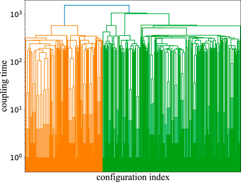
Figure 3. Dendrogram of configurations in the partial-survey approximation for the three-dimensional Edwards–Anderson model with parallel updates at $T=3.90\gtrsim T_{\text{coup}}$ and with ${\mathcal{N}}_0=512$. Any starting set with representative configurations in the two main branches (orange, green) gives the same coupling time, explaining the success of the partial survey.

All the figures shown below represent results averaged over 4,096 realizations of interactions, independent of $N$, with error bars indicating sample fluctuations from these realizations. The first results for the three-dimensional Edwards–Anderson model are presented in the two panels of Figure 4, which show the estimated mean coupling time for the partial-survey approximation under the parallel and random updates. Although the two updates differ in the high-temperature limit, both exhibit a $N\log N$ behavior for system size $N$ at sufficiently high but finite temperatures. As the temperature decreases, the behavior of the $N$ dependence of the mean coupling time changes from slow to fast increase at a certain temperature. There is a slight, yet significant, difference in the transition temperature between the two updates, with a lower transition temperature observed for the parallel updates. This illustrates that coupling has no direct thermodynamic significance.

Figure 4

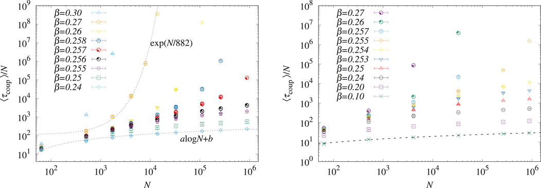
Figure 4. System-size $N$ dependence of the mean coupling time at various inverse temperatures in the three-dimensional Edwards–Anderson model. Left: Parallel update. Right: Random update.

Figure 5 presents finite-size scaling plots of the mean coupling time for the three-dimensional Edwards–Anderson model, comparing both the parallel and random updates. The plot demonstrates that the scaling works well when the appropriate scaling parameters are chosen. This is consistent with the above argument that the transition temperatures, $T_{\text{coup}}$ or ${\beta }_{\text{coup}}$, are significantly different for the two update rules. In contrast, the precision of the scaling exponents, $\varphi$ and $\omega$, is not as precise as that of the transition temperature, and it can be considered that these two rules yield almost the same values for these exponents. It remains unclear whether these exponents have a meaning analogous to the critical exponents of a second-order transition. Of particular interest is the exponent $\omega$, which represents the divergence of the characteristic scale as it approaches the transition temperature. Our results suggest that this exponent has the same value on both the high- and low-temperature sides of the transition temperature. This is comparable to the correlation length exponent.

Figure 5

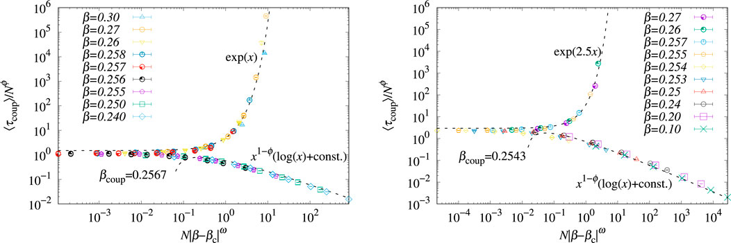
Figure 5. Finite-size scaling plot of the mean coupling time in the three-dimensional Edwards–Anderson model. Left: Parallel updates ($\omega \simeq 1.7$, $\varphi \simeq 1.7$, and ${\beta }_{\text{coup}}\simeq 0.2567$). Right: Random updates ($\omega \simeq 1.84$, $\varphi \simeq 1.70$, and ${\beta }_{\text{coup}}\simeq 0.2543$). Two dotted lines in each panel represent the expected high- and low-temperature asymptotic forms of the scaling function.

An analogous scaling analysis for the two-dimensional Edwards–Anderson model is shown in Figure 6. The left panel is the analysis result of our own numerical simulations using the sublattice parallel update, while the right panel presents the scaling analysis based on numerical data using the random update from [4]. In both cases, the scaling is consistent with a phase transition in the mean coupling time. As observed in the three-dimensional model, $T_{\text{coup}}$ depends on the underlying Markov chain, with a lower transition temperature for the parallel update. The scaling exponents depend on the dimensionality. However, the proper scaling variable may not be the number of spins, $N$, used here, but rather the linear dimension $L$. This suggests that the value of the exponents may depend on the dimensionality through the relationship $N=L^d$.

Figure 6

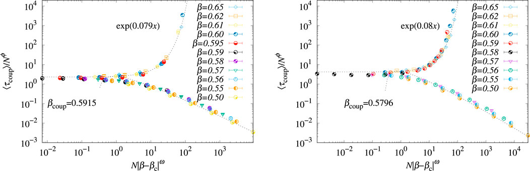
Figure 6. Finite-size scaling plot of the mean coupling time in the two-dimensional Edwards–Anderson model. Left: Parallel update (our simulations). The obtained parameters are $\omega \simeq 1.4$, $\varphi \simeq 1.95$, and ${\beta }_{\text{coup}}\simeq 0.5915$. Right: Random updates (original data of Ref. [4]). The obtained parameters are $\omega \simeq 1.4$, $\varphi \simeq 1.95$, and ${\beta }_{\text{coup}}\simeq 0.5796$. Two dotted lines in each panel represent the expected high- and low-temperature asymptotic forms of the scaling function.

3.3 Path coupling and damage spreading for spin glasses

Table 1 summarizes the key temperatures discussed in previous sections, including $T_{\text{path}}$ and $T_{\text{coup}}$, as well as previously estimated results for $T_{\text{SG}}$ and $T_{\text{Griffiths}}$. This table demonstrates the differences in transition temperatures for both two- and three-dimensional Edwards–Anderson models, providing a detailed overview of the coupling and spin-glass transitions.

Table 1

Table 1. Spin-glass transition and coupling temperatures for the Edwards–Anderson model in two and three dimensions. $T_{\text{SG}}$ is the numerical estimate from Refs. [3, 30] in three dimensions and is expected [8, 34] to vanish in two dimensions. $T_{\text{coup}}$ is from Figures 5, 6, and $T_{\text{Griffiths}}$ is the Curie temperature of the ferromagnetic Ising model. Finally, $T_{\text{path}}$ is from Equation 8.

On the one hand, path coupling demonstrates that above $T_{\text{path}}$, the uniform contraction between neighboring configurations leads to fast coupling. Below $T_{\text{path}}$, there are spins $k$ (for example, those with $h_k=0$) for which, at least initially, there is no such contraction. Nevertheless, as our numerical simulations show, fast $N\text{log}N$ coupling also takes place in the window $T_{\text{coup}}<T<T_{\text{path}}$. The absence of a regime change at $T_{\text{path}}$ can be illustrated, in the language of damage spreading, by following the mean damage as a function of time for two configurations that initially, at time $t=0$, are neighboring. Above $T_{\text{path}}$, the mean damage decreases exponentially for all times (see inset of Figure 7), whereas for $T<T_{\text{coup}}$, it increases rapidly. In the window $T_{\text{coup}}\lesssim T\lesssim T_{\text{path}}$, the mean damage initially increases, as expected, but then turns around and again vanishes exponentially. This turning point seems to occur when the damage reaches a certain size, which grows as the temperature approaches $T_{\text{coup}}$. This behavior can be understood in analogy with the characteristic diverging scale $N*(\beta )$ in the finite-size scaling analysis of Equation 5, which suggests a picture similar to a critical phase transition, where the threshold damage size corresponds to the diverging scale near $T_{\text{coup}}$.

Figure 7

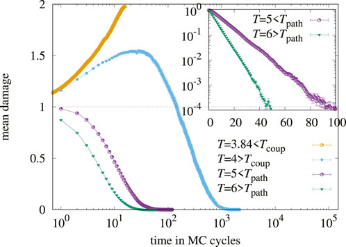
Figure 7. Damage evolution over time for two states differing by a Hamming distance of 1 as initial conditions in random updates of the three-dimensional Edwards–Anderson model. The size is $N=64^3$, and the four temperatures shown are above and below both $T_{\text{path}}$ and $T_{\text{coup}}$. The inset shows the same plot on a semi-log scale.

4 Coupling in hard spheres

In this section, we examine coupling for the hard-sphere system of statistical mechanics. For concreteness, we concentrate on the two-dimensional hard-disk model, which was the object of the historically first study using Markov chains [43]. The model has created an unabating series of works in mathematics, physics, and chemistry [40]. After an introduction to the model and to the Metropolis algorithm [35] that we will mostly consider, we review the very few known exact results on the model (Section 4.1) and then move on to the analysis of path coupling (Section 4.2) and to numerical calculations leading up to our scaling analysis. We finally discuss, following Ref. [32], what, precisely, the behavior of the algorithm teaches us about the physics of the hard-disk model (Section 4.3).

The model describes $N$ disks of radius $\sigma$ in a rectangular box with periodic boundary conditions. For simplicity, we assume the box to be a square of side length $L$. The center position of disk $k$ is given by ${\mathbf{x}}_k=(x_k,y_k)$ and in a “legal” configuration, any two disks cannot overlap (get closer than $2\sigma$), periodic boundary conditions being accounted for. The sample space $\mathrm{\Omega }$ is now continuous, and the statistical weight of a configuration $\mathbf{X}=\{{\mathbf{x}}_1,\dots ,{\mathbf{x}}_N\}$ is given by

$\pi \left(\mathbf{X}\right)=\left\{\begin{array}{cc}1\hfill & \text{if\hspace{0.17em}}\mathbf{X}\text{is\hspace{0.17em}legal}\hfill \\ 0\hfill & \text{else}\hfill \end{array}\right.,$

where, for simplicity, we have omitted the Cartesian $2N$-dimensional measure. The control parameter of this model is the density $\eta =N\pi {\sigma }^2/L^2$, the fraction of occupied space to the volume of the box.

We consider the “global” Metropolis algorithm: At each time step, and starting from a configuration $\mathbf{X}(t)=\{{\mathbf{x}}_1,\dots ,{\mathbf{x}}_N\}$, one random disk $k$ among the $N$ disks is sampled. A move of disk $k$ from ${\mathbf{x}}_k$ to a random position inside the simulation box ${\mathbf{x}}_k^{\prime }=\left[\mathtt{ran}(0,L),\mathtt{ran}(0,L)\right]$ is attempted. If the configuration ${\mathbf{X}}^{\prime }$, in which $\mathbf{x}$ is replaced by ${\mathbf{x}}^{\prime }$ is legal, the move is accepted and otherwise rejected:

$\mathbf{X}\left(t+1\right)=\left\{\begin{array}{cc}\{{\mathbf{x}}_1,\dots ,{\mathbf{x}}_{k-1},{\mathbf{x}}_k^{\prime },{\mathbf{x}}_{k+1},\dots ,{\mathbf{x}}_N\}\hfill & \mathrm{i}\mathrm{f}\mathrm{l}\mathrm{e}\mathrm{g}\mathrm{a}\mathrm{l}\hfill \\ \mathbf{X}\left(t\right)\hfill & \text{otherwise}\hfill \end{array}\right..$

Here, the new position is chosen within a square-shaped periodic window of length $L$ around the current position, whereas in the local Metropolis algorithm, the window size usually has a length on the scale of the inter-particle distance [36].

The random-share coupling for the global Metropolis algorithm uses the following random element:

${\mathbf{\Upsilon }}_t=\{k,{\mathbf{x}}^{\prime }=\{x,y\}\}=\{\underset{\text{particle}\text{index}k}{\underbrace{\mathtt{n}\mathtt{r}\mathtt{a}\mathtt{n}(1,N)}},\underset{\text{proposed}\text{position}{\mathbf{x}}^{\prime }={\mathbf{x}}_k\left(t+1\right)}{\underbrace{\{\mathtt{r}\mathtt{a}\mathtt{n}(0,L),\mathtt{r}\mathtt{a}\mathtt{n}(0,L)\}}}\}.(9)$

This coupling has been considerably refined [31, 32].

4.1 Rigorous results for the thermodynamics of hard spheres

Rigorous results on hard-disk (and hard-sphere) models are very few. It is known that the close-packing density $\eta =\pi /(2\sqrt{3})$ in two dimensions is characterized by the hexagonal packing [24]. It thus corresponds to an essentially unique configuration that has long-range orientational and positional order. For densities below the close-packing density, the absence of long-range positional order was established rigorously [50] so that there is no crystal (with long-range orientational and positional order) below close packing. Indications for a phase transition were first found in the 1960s [1, 40]. The existence of two phase transitions and of three phases (liquid, hexatic, and solid) as a function of density is now well accepted [5, 40]. As in the Edwards–Anderson model (where the temperature $T$ replaces the inverse of the density $\eta$ as a control parameter), a rigorous proof of a transition away from close packing is still lacking. At low finite densities, the convergence of the virial expansion was proven early on [38], establishing the existence of the liquid phase. It extends up to a density $\eta =0.70$ and is followed by a window of coexisting liquid and hexatic regions (see Table 2 below).

Table 2

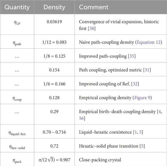
Table 2. Densities in the hard-disk system (see Equation 1 of Ref. [40]) for common definitions of densities). The homogeneous liquid phase empirically extends to a density of 0.70. The homogeneous hexatic phase is from 0.716 to 0.72. The density range from 0.70 to 0.716 corresponds to phase separation.

4.2 Path coupling and scaling plots for hard disks

We now consider path coupling for hard disks, using the random map based on Equation 9 and a Hamming metric that counts the number of different disk positions in any two configurations. Let ${\mathbf{X}}^A$ and ${\mathbf{X}}^B$ be two neighboring hard-disk configurations that differ in the position of disk $j$ only (see Figure 8). Simplifying a coupling from Ref. [35], we use as the common random element $\{k,\mathbf{\Upsilon }\}$ the disk $k$ to be updated and its new position, both identical for ${\mathbf{X}}^A$ and ${\mathbf{X}}^B$. With probability $1/N$, the disk $j$ is moved (that is, $k=j$). The move is accepted in both configurations if it stays away (by $2\sigma$) from the “halo” of all remaining disks in both configurations. This yields the probability of decreasing the Hamming distance from 1 to 0:

$p_{1\to 0}\ge \frac{1}{N}\left(1-\frac{N-1}{N}4\eta \right).(10)$

Figure 8

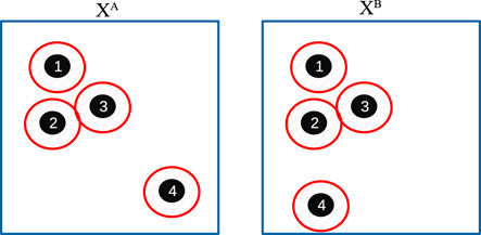
Figure 8. Hard-disk configurations, differing only in disk $j=4$. Under the random-share coupling, the difference disappears if the disk $j$ is moved to a position outside the “halo” of other disks (see Equation 10). It is increased to two if the move of disk $k\ne j$ would overlap with $j$ in only one of the configurations (see Equation 11). Disks of radius $\sigma$ are shown with their $2\sigma$ halos.

On the other hand, the Hamming distance can be increased from 1 to 2 if a disk different from $j$ is moved less than $2\sigma$ away (that is, into the halo), of disk $j$ in one configuration but not in the other. The probability of increasing the Hamming distance from one to two can thus be bounded as:

$p_{1\to 2}\le \frac{N-1}{N}\left(\frac{8}{N}\eta \right),(11)$

where the factor $8\eta /N$ on the rhs arises from the difference between two “halos” of area $4\pi {\sigma }^2$ for each of the disks j in the two configurations.

Again, for $p_{1\to 0}>p_{1\to 2}$, the expected Hamming distance between $A$ and $B$ decreases after one step, for any two neighboring disk configurations, which can be assured for

$\eta <{\eta }_{\text{path}}=\frac{1}{12}.(13)$

It follows [13] that the Hamming distance between configurations $A$ and $B$ that differ in the position of only one disk decreases in expectation at each step if the density is smaller than $1/12$.

As with the Edwards–Anderson model, we now analyze the mean coupling time of the two-dimensional hard-disk model under the global Metropolis algorithm with the random-share coupling of Equation 9. In this case, we reanalyze the data obtained in Ref. [4], which we replot on the lhs of Figure 9. The analogous scaling ansatz again provides an excellent fit of the data. The critical exponents do not differ significantly from those found in the Edwards–Anderson model, suggesting the possibility of some underlying universality. However, uncovering the intricate physical picture behind this similarity remains an open question for future research. It should be noted that these critical exponents are not directly related to the critical phenomena of physical systems in the conventional sense. Rather, they characterize the “phase transition” in computational algorithms associated with the coupling of Markov chains. From an algorithmic perspective, these exponents are of significant interest as they provide insight into the inherent challenges in achieving fast coupling.

Figure 9

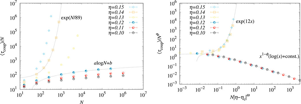
Figure 9. Left: System-size dependence of the mean coupling time at various densities in two-dimensional hard disks (data from Ref. [4]). Right: Finite-size scaling plot of the coupling time with parameters $\omega \simeq 1.6$, $\varphi \simeq 1.75$, and ${\eta }_{\text{c}}\simeq 0.128$. The two dotted lines represent the expected high- and low-density asymptotic forms of the scaling function.

4.3 Advanced hard-disk couplings, physical implications

The coupling approach to the hard-disk system has been intensely studied in recent years, and the random-share coupling of Equation 9 only provides the simplest possible choice. A number of refined couplings have been proposed. The one proposed in Ref. [35] moves disks differently for the configuration ${\mathbf{X}}^A$ and ${\mathbf{X}}^B$ and reaches a path-coupling density of $1/8$ (see Table 2 for an overview). Building on this coupling, optimizing the metric reaches a limiting density of 0.154, which was later improved for a different algorithm to $1/6$. In addition to these rigorous bounds, numerical evidence for the birth–death algorithm [56] points to a coupling density of $\sim 0.3$ [4]. These densities, and especially the rigorously proven ones, are still quite far from the “empirical” transition density $\eta \sim 0.70$ of the liquid phase, which was only in recent years understood to be toward a hexatic, and which bounds on a region $\eta \in [0.7,0.76]$ without a homogeneous solution, and then giving rise to a mixture of the hexatic and the liquid.

The crucial connection between fast coupling (thus, fast mixing) and physical ordering was made for the hard-sphere case in Ref. [32], where it was proven that $\mathtt{O}(N\text{log}N)$ random steps of the global Metropolis algorithm are insufficient to construct configurations with any kind of long-range order. Fast mixing of a single-particle algorithm, even a non-local one, thus implies that the resulting configuration (which is practically in equilibrium) has exponential spatial correlation functions. This, to all intents and purposes, shows the extension of the liquid phase. We believe that it does not, however, prove the convergence of the virial expansion [38] because of the possibility of a liquid–liquid phase transition, which cannot be captured in a mixing-time argument.

5 Conclusion

In this article, we have discussed the computational aspects of two of the most challenging models in statistical physics, namely, the Edwards–Anderson model and the hard-disk model. In both these models, there are almost no rigorous results about the phase transitions in non-trivial physical dimensions, that is, above two dimensions for the spin model and above one dimension (away from close packing) for the particle system. Further connections are that the computational algorithms are mostly derivatives of the local-move heat-bath or Metropolis algorithm in both cases. Cluster algorithms have been developed for both systems [21, 34], but they have not really been useful in the physically interesting dimensions. Finally, the two models are united by the fact that they are truly challenging in their physical interpretation: For the Edwards–Anderson model, for a long time, even empirically, there was only a very rough agreed-on value of the transition temperature from the high-temperature paramagnetic phase, which was considerably sharpened in recent times only (see Table 1). No agreement has been reached on the nature of the low-temperature phase. For the hard-disk model, the now agreed-on transition scenario [5] was proposed only a decade ago, after more than 50 years of intense simulation. In that model, even the simplest algorithm, the local Metropolis algorithm, faces extreme challenges, as its irreducibility and ergodicity cannot be guaranteed in the constant-volume ensemble [11, 33].

In this context, the coupling approach provides an interesting yet incomplete view of the high-temperature/low-density phases. In the Edwards–Anderson model, one can easily establish the existence of a path-coupling temperature (see Equation 8), which we think provides a rigorous upper bound for the extension of the paramagnetic phase. For the hard-disk model, the program has been followed through completely, and the coupling result is the currently best lower bound for the extension of the liquid phase. It is fascinating how a result on the speed of a Monte Carlo algorithm can be derived from the behavior of two Markov chains (that is, from coupling) and can then be turned into a statement on the phase behavior. This fascination was sensed early on in the literature on damage spreading that, as we discussed, naturally connects to the path-coupling approach.

Damage spreading has created an extensive literature in physics, but, as we pointed out, that literature has concentrated on the specific random-share protocol, which gives the very low bounding density of Equation 12 when translated to the hard-disk context. In particle systems, there has been much progress from improved couplings and optimized metrics (see Table 2), which we hope can be ported to spin glasses and, more generally, to disordered systems. It would be interesting to see whether our scaling approach can be applied to these more advanced couplings.

Data availability statement

The raw data supporting the conclusions of this article will be made available by the authors, without undue reservation.

Author contributions

KH: writing–original draft and writing–review and editing. WK: writing–original draft and writing–review and editing.

Funding

The author(s) declare that financial support was received for the research, authorship, and/or publication of this article. This research was supported by a grant from the Simons Foundation (Grant 839534, MET). This work was also supported by JSPS KAKENHI Grant Nos. 23H01095, and JST Grant Number JPMJPF2221. This research was conducted within the context of the International Research Project “Non-Reversible Markov chains, Implementations and Applications.”

Acknowledgments

We thank J. L. Lebowitz for an inspiring discussion. KH would like to thank the Ecole Normale Supérieure, ENS, for their kind hospitality during a research stay, which provided a productive environment and variable support for the completion of this work. The authors thank the Supercomputer Center, the Institute for Solid State Physics, and the University of Tokyo for the use of the facilities.

Conflict of interest

The authors declare that the research was conducted in the absence of any commercial or financial relationships that could be construed as a potential conflict of interest.

Generative AI statement

The author(s) declare that no Generative AI was used in the creation of this manuscript.

Publisher’s note

All claims expressed in this article are solely those of the authors and do not necessarily represent those of their affiliated organizations, or those of the publisher, the editors and the reviewers. Any product that may be evaluated in this article, or claim that may be made by its manufacturer, is not guaranteed or endorsed by the publisher.

References

1. Alder BJ, Wainwright TE. Phase transition in elastic disks. Phys Rev (1962) 127:359–61. doi:10.1103/PhysRev.127.359

CrossRef Full Text | Google Scholar

2. Aldous D, Diaconis P. Shuffling cards and stopping times. The Am Math Monthly (1986) 93:333–48. doi:10.2307/2323590

CrossRef Full Text | Google Scholar

3. Baity-Jesi M, Baños RA, Cruz A, Fernandez LA, Gil-Narvion JM, Gordillo-Guerrero A, et al. Critical parameters of the three-dimensional Ising spin glass. Phys Rev B (2013) 88:224416. doi:10.1103/PhysRevB.88.224416

CrossRef Full Text | Google Scholar

4. Bernard EP, Chanal C, Krauth W. Damage spreading and coupling in Markov chains. EPL (Europhysics Letters) (2010) 92:60004. doi:10.1209/0295-5075/92/60004

CrossRef Full Text | Google Scholar

5. Bernard EP, Krauth W. Two-step melting in two dimensions: first-order liquid-hexatic transition. Phys Rev Lett (2011) 107:155704. doi:10.1103/PhysRevLett.107.155704

PubMed Abstract | CrossRef Full Text | Google Scholar

6. Berretti A. Some properties of random Ising models. J Stat Phys (1985) 38:483–96. doi:10.1007/BF01010473

CrossRef Full Text | Google Scholar

7. Bhatt RN, Young AP. Search for a transition in the three-dimensional ±J Ising spin-glass. Phys Rev Lett (1985) 54:924–7. doi:10.1103/PhysRevLett.54.924

PubMed Abstract | CrossRef Full Text | Google Scholar

8. Bhatt RN, Young AP. Numerical studies of Ising spin glasses in two, three, and four dimensions. Phys Rev B (1988) 37:5606–14. doi:10.1103/PhysRevB.37.5606

PubMed Abstract | CrossRef Full Text | Google Scholar

9. Bieche L, Uhry JP, Maynard R, Rammal R. On the ground states of the frustration model of a spin glass by a matching method of graph theory. J Phys A: Math Gen (1980) 13:2553–76. doi:10.1088/0305-4470/13/8/005

CrossRef Full Text | Google Scholar

10. Boettcher S. Stiffness of the Edwards-Anderson model in all dimensions. Phys Rev Lett (2005) 95:197205. doi:10.1103/PhysRevLett.95.197205

PubMed Abstract | CrossRef Full Text | Google Scholar

11. Böröczky K. Über stabile Kreis-und Kugelsysteme. Ann Univ Sci Budapest Eötvös Sect Math (1964) 7:79–82.

Google Scholar

12. Bray AJ, Moore MA. Lower critical dimension of Ising spin glasses: a numerical study. J Phys C: Solid State Phys (1984) 17:L463–8. doi:10.1088/0022-3719/17/18/004

CrossRef Full Text | Google Scholar

13. Bubley R, Dyer M. Path coupling: a technique for proving rapid mixing in Markov chains. In: 2013 IEEE 54th Annual Symposium on Foundations of Computer Science, Los Alamitos, CA, USA: IEEE Computer Society (1997). 223.

Google Scholar

14. Campbell I, de Arcangelis L. On the damage spreading in Ising spin glasses. Physica A: Stat Mech its Appl (1991) 178:29–43. doi:10.1016/0378-4371(91)90073-l

CrossRef Full Text | Google Scholar

15. Chanal C, Krauth W. Renormalization group approach to exact sampling. Phys Rev Lett (2008) 100:060601. doi:10.1103/PhysRevLett.100.060601

PubMed Abstract | CrossRef Full Text | Google Scholar

16. Chanal C, Krauth W. Convergence and coupling for spin glasses and hard spheres. Phys Rev E (2010) 81:016705. doi:10.1103/PhysRevE.81.016705

PubMed Abstract | CrossRef Full Text | Google Scholar

17. Creutz M. Monte Carlo study of quantized SU(2) gauge theory. Phys Rev D (1980) 21:2308–15. doi:10.1103/PhysRevD.21.2308

CrossRef Full Text | Google Scholar

18. Derrida B, Weisbuch G. Dynamical phase transitions in 3-dimensional spin glasses. EPL (1987) 4:657–62. doi:10.1209/0295-5075/4/6/004

CrossRef Full Text | Google Scholar

19. Ding J, Lubetzky E, Peres Y. The mixing time evolution of Glauber dynamics for the mean-field Ising model. Commun Math Phys (2009) 289:725–64. doi:10.1007/s00220-009-0781-9

CrossRef Full Text | Google Scholar

20. Doeblin W. Exposé de la Théorie des chaînes simples constantes de Markoff à un nombre fini d’états. Rev Math Union Interbalkanique (1938) 2:77.

Google Scholar

21. Dress C, Krauth W. Cluster algorithm for hard spheres and related systems. J Phys A: Math Gen (1995) 28:L597–L601. doi:10.1088/0305-4470/28/23/001

CrossRef Full Text | Google Scholar

22. Dyer M, Sinclair A, Vigoda E, Weitz D. Mixing in time and space for lattice spin systems: a combinatorial view. Random Struct Algorithms (2004) 24:461–79. doi:10.1002/rsa.20004

CrossRef Full Text | Google Scholar

23. Edwards SF, Anderson PW. Theory of spin glasses. J Phys F: Metal Phys (1975) 5:965–74. doi:10.1088/0305-4608/5/5/017

CrossRef Full Text | Google Scholar

24. Fejes L. Über einen geometrischen Satz. Mathematische Z (1940) 46:83–5. doi:10.1007/BF01181430

CrossRef Full Text | Google Scholar

25. Fröhlich J, Imbrie JZ. Improved perturbation expansion for disordered systems: beating Griffiths singularities. Commun Math Phys (1984) 96:145–80. doi:10.1007/BF01240218

CrossRef Full Text | Google Scholar

26. Geman S, Geman D. Stochastic relaxation, Gibbs distributions, and the Bayesian restoration of images. IEEE Trans Pattern Anal Mach Intell (1984) PAMI-6:721–41. doi:10.1109/tpami.1984.4767596

PubMed Abstract | CrossRef Full Text | Google Scholar

27. Glauber RJ. Time-dependent statistics of the Ising model. J Math Phys (1963) 4:294–307. doi:10.1063/1.1703954

CrossRef Full Text | Google Scholar

28. Griffeath D. A maximal coupling for Markov chains. Z fr̈ Wahrscheinlichkeitstheorie Verwandte Gebiete (1975) 31:95–106. doi:10.1007/bf00539434

CrossRef Full Text | Google Scholar

29. Griffiths RB. Nonanalytic behavior above the critical point in a random Ising ferromagnet. Phys Rev Lett (1969) 23:17–9. doi:10.1103/PhysRevLett.23.17

CrossRef Full Text | Google Scholar

30. Hasenbusch M, Pelissetto A, Vicari E. Critical behavior of three-dimensional Ising spin glass models. Phys Rev B (2008) 78:214205. doi:10.1103/PhysRevB.78.214205

CrossRef Full Text | Google Scholar

31. Hayes TP, Moore C. Lower bounds on the critical density in the hard disk model via optimized metrics. arXiv:1407.1930 (2014). doi:10.48550/arXiv.1407.1930

CrossRef Full Text | Google Scholar

32. Helmuth T, Perkins W, Petti S. Correlation decay for hard spheres via Markov chains. The Ann Appl Probab (2022) 32. doi:10.1214/21-aap1728

PubMed Abstract | CrossRef Full Text | Google Scholar

33. Höllmer P, Noirault N, Li B, Maggs AC, Krauth W. Sparse hard-disk packings and local Markov chains. J Stat Phys (2022) 187:31. doi:10.1007/s10955-022-02908-4

CrossRef Full Text | Google Scholar

34. Houdayer J. A cluster Monte Carlo algorithm for 2-dimensional spin glasses. The Eur Phys J B - Condensed Matter Complex Syst (2001) 22:479–84. doi:10.1007/PL00011151

CrossRef Full Text | Google Scholar

35. Kannan R, Mahoney MW, Montenegro R. Rapid mixing of several Markov chains for a hard-core model. Proc 14th Annual ISAAC (Springer, Berlin, Heidelberg), Lecture Notes Computer Sci (2003) 663–75. doi:10.1007/978-3-540-24587-2_68

CrossRef Full Text | Google Scholar

36. Krauth W. Statistical mechanics: algorithms and computations. Oxford University Press (2006).

Google Scholar

37. Landau D, Binder K. A guide to Monte Carlo simulations in statistical physics. Cambridge University Press (2013).

Google Scholar

38. Lebowitz JL, Penrose O. Convergence of virial expansions. J Math Phys (1964) 5:841–7. doi:10.1063/1.1704186

CrossRef Full Text | Google Scholar

39. Levin DA, Peres Y, Wilmer EL. Markov chains and mixing times. American Mathematical Society (2008).

Google Scholar

40. Li B, Nishikawa Y, Höllmer P, Carillo L, Maggs AC, Krauth W. Hard-disk pressure computations—a historic perspective. J Chem Phys (2022) 157:234111. doi:10.1063/5.0126437

PubMed Abstract | CrossRef Full Text | Google Scholar

41. Martinelli F. Lectures on Glauber dynamics for discrete spin models. In: P Bernard, editor Lectures on Probability Theory and Statistics: Ecole d’Eté de Probabilités de Saint-Flour XXVII - 1997. Berlin, Heidelberg: Springer Berlin Heidelberg (1999). p. 93–191.

CrossRef Full Text | Google Scholar

42. McMillan WL. Domain-wall renormalization-group study of the three-dimensional random Ising model. Phys Rev B (1984) 30:476–7. doi:10.1103/PhysRevB.30.476

CrossRef Full Text | Google Scholar

43. Metropolis N, Rosenbluth AW, Rosenbluth MN, Teller AH, Teller E. Equation of state calculations by fast computing machines. J Chem Phys (1953) 21:1087–92. doi:10.1063/1.1699114

CrossRef Full Text | Google Scholar

44. Mezard M, Parisi G, Virasoro M. Spin glass theory and beyond. World Scientific (1986). doi:10.1142/0271

CrossRef Full Text | Google Scholar

45. Nattermann T, Villain J. Random-field ising systems: a survey of current theoretical views. Phase Transitions (1988) 11:5–51. doi:10.1080/01411598808245480

CrossRef Full Text | Google Scholar

46. Ogielski AT. Dynamics of three-dimensional Ising spin glasses in thermal equilibrium. Phys Rev B (1985) 32:7384–98. doi:10.1103/PhysRevB.32.7384

PubMed Abstract | CrossRef Full Text | Google Scholar

47. Ogielski AT, Morgenstern I. Critical behavior of three-dimensional Ising spin-glass model. Phys Rev Lett (1985) 54:928–31. doi:10.1103/PhysRevLett.54.928

PubMed Abstract | CrossRef Full Text | Google Scholar

48. Propp JG, Wilson DB. Exact sampling with coupled Markov chains and applications to statistical mechanics. Random Structures and Algorithms (1996) 9:223–52. doi:10.1002/(sici)1098-2418(199608/09)9:1/2<223::aid-rsa14>3.3.co;2-r

CrossRef Full Text | Google Scholar

49. Randall D, Winkler P. Mixing points on an interval. In: C Demetrescu, R Sedgewick, and R Tamassia, editors. Proceedings of the seventh workshop on algorithm engineering and experiments and the second workshop on analytic algorithmics and combinatorics, ALENEX/ANALCO 2005. Vancouver, BC, Canada: SIAM (2005). p. 218–21.

Google Scholar

50. Richthammer T. Lower bound on the mean square displacement of particles in the hard disk model. Commun Math Phys (2016) 345:1077–99. doi:10.1007/s00220-016-2584-0

CrossRef Full Text | Google Scholar

51. Franz S, Parisi G, Virasoro MA. Interfaces and lower critical dimension in a spin glass model. J Phys France (1994) 4:1657–67. doi:10.1051/jp1:1994213

CrossRef Full Text | Google Scholar

52. Sherrington D, Kirkpatrick S. Solvable model of a spin-glass. Phys Rev Lett (1975) 35:1792–6. doi:10.1103/PhysRevLett.35.1792

CrossRef Full Text | Google Scholar

53. Stanley HE, Stauffer D, Kertész J, Herrmann HJ. Dynamics of spreading phenomena in two-dimensional Ising models. Phys Rev Lett (1987) 59:2326–8. doi:10.1103/PhysRevLett.59.2326

PubMed Abstract | CrossRef Full Text | Google Scholar

54. Talagrand M. Spin glasses: a challenge for mathematicians: cavity and mean field models. In: Ergebnisse der Mathematik und ihrer Grenzgebiete. 3. Folge A Series of Modern Surveys in Mathematics. Springer (2003).

Google Scholar

55. Thomas CK, Middleton AA. Exact algorithm for sampling the two-dimensional Ising spin glass. Phys Rev E (2009) 80:046708. doi:10.1103/PhysRevE.80.046708

PubMed Abstract | CrossRef Full Text | Google Scholar

56. Wilson DB. How to couple from the past using a read-once source of randomness. Random Structures and Algorithms (2000) 16:85–113. doi:10.1002/(SICI)1098-2418(200001)16:1⟨85::AID-RSA6⟩3.0.CO;2-H

CrossRef Full Text | Google Scholar