Exponential series approximation of the SIR epidemiological model

Introduction: The SIR (Susceptible-Infected-Recovered) model is one of the simplest and most widely used frameworks for understanding epidemic outbreaks.

Methods: A second-order dynamical system for the R variable is formulated using an infinite exponential series expansion, and a recursion relation is established between the series coefficients. A numerical approximation scheme for the R variable is also developed.

Results: The proposed numerical method is compared to a double exponential (DE) nonlinear approximate analytic solution, which reveals two coupled timescales: a relaxation timescale, determined by the ratio of the model’s time constants, and an excitation timescale, dictated by the population size. The DE solution is applied to estimate model parameters for a well-known epidemiological dataset—the boarding school flu outbreak.

Discussion: From a theoretical standpoint, the primary contribution of this work is the derivation of an infinite exponential, Dirichlet, series for the model variables. Truncating the series yields a finite approximation, known as a Prony series, which can be interpreted as a sequence of coupled exponential relaxation processes, each with a distinct timescale. This apparent complexity can be approximated well by the DE solution, which appears to be of main practical interest.

1 Introduction

Epidemic models have undergone steady development during the last 100 years. The SIR model, short for Susceptible-Infectious-Recovered model, is a fundamental framework in epidemiology used to describe the spread of infectious diseases within a population. Developed by Kermack and McKendrick in the early 20th century [1], the SIR model categorizes individuals into three compartments: Susceptible (S), those who can contract the disease; Infectious (I), those who have contracted the disease and can transmit it to others; and Recovered (R), those who have recovered from the disease and are assumed to be immune. The SIR model is used to model epidemic outbreaks (see the monograph of Martcheva [2] or [3]). By modeling the rates of transition between these compartments, the SIR model provides insights into the dynamics of epidemic outbreaks, helping predict the spread and eventual decline of infections. It should be noted that the original model derived by Kermack and McKendrick was formulated in terms of convolution integrals, while the more popular form used in the present literature is actually only its simplified case.

The SIR model is one of the simplest examples of dynamical system with a positive and a negative feedback loops. That is, the model features competing excitation and relaxation processes. The SIR model has an universal applicability in epidemiology as well as in different areas of social sciences – information spread in social networks, behavior and influence adoption, social movements and protests, etc. [5]. For example, in social networks individuals in the network can be categorized as susceptible (not yet informed), infectious (spreading the information), or recovered (informed but no longer spreading).

Kendall [6] derived the parametric solution for the $R$-variable, however, he could not formulate the complete parametric solution since during his time the Lambert W and Wright Omega functions were not available. The parametric solution of the SIR model through the S-variable was derived in [7] Barlow and Weinstein derived a power series for the S-variable and introduced rational convergents on the positive half-plane [8]. A different approximation scheme was introduced in [9]. Analytic Taylor series have been obtained in [10] but they are purely of theoretical interest. An inverse parametric solution for the I-variable was obtained independently by the present author [10, 11] and Kudryashov al. [12]. An equivalent differential system has been obtained in [13]. The modern literature on the applications of the SIR model has become quite extensive in view of the applications to the COVID-10 pandemic and will not be reviewed here.

The main contribution of the present manuscript is to give an analytical solution of the SIR model as infinite exponential (i.e. general Dirichlet) series. Upon truncation the solution produces a finite Prony series, which can be of some practical interest. The Prony series expression is a mathematical tool used primarily to model viscoelastic materials, capturing their time-dependent behavior through a sum of exponential terms. Each term represents a distinct relaxation process with specific relaxation times and moduli. This series is particularly useful in engineering and material science for simulating and predicting the performance of polymers, rubbers, and biological tissues. The article further derives the double exponential approximate analytical solution of the SIR model. Finally, the third contribution of the article is a Newtonian iteration schema for the R-variable.

2 Preliminaries of the SIR model

The contemporary formulation of the model can be found in [2]. The SIR model is built on several simplifying assumptions [4]. The dynamical formulation of the model comprises a set of three ordinary differential equations ODEs Equations 1–3:

$\frac{d}{dt}S\left(t\right)=-\frac{\beta }{N}S\left(t\right)I\left(t\right)(1)$

$\frac{d}{dt}I\left(t\right)=\frac{\beta }{N}S\left(t\right)I\left(t\right)-\gamma I\left(t\right)(2)$

$\frac{d}{dt}R\left(t\right)=\gamma I\left(t\right)(3)$

By construction, the model assumes a constant overall population $N=S(t)+I(t)+R(t)$ [1]. The interpretation of the parameters is that a disease carrier infects on average $\beta$ individuals per day, for an average time of $1/\gamma$ days. The $\beta$ parameter is called disease transmission rate, while $\gamma$ – recovery rate. The average number of infections arising from an infected individual is then modeled by the number $R_0=\beta /\gamma$, the basic reproduction number. Typical initial conditions are $S(0)=S_0,I(0)=I_0,R(0)=0$ [1]. The model is strictly valid for an isolated population of known size N. This is in practice seldom the case; therefore, in many publications, the population size N is absorbed in the $\beta$ time constant. Due to the constant population size N (i.e the first integral) only two variables are independent.

2.1 On two useful special functions

The theory of the SIR model is closely related to two special functions – the Lambert W function and the Wright’s $\mathrm{\Omega }$ function, which is less well-known and can be expressed as a composition of the W function.

The Lambert W function is defined implicitly by the functional equation

$W\left(z\right)e^{W\left(z\right)}≕z,z\in \mathbb{C}(4)$

and as such is the simplest example of a root of an exponential polynomial. Properties of the function are surveyed in [14]. It is particularly useful in solving equations where the variable appears both in the base and the exponent, and it finds applications in various fields, such as combinatorics, physics, biochemistry, and complex analysis. Applications in physics include the Wien’s displacement law; in biochemistry – the Michaelis-Menten kinetic equation, etc. In general, the W function is multivalued. Analytically continued on the complex plane, the function has a countably infinite number of complex-valued branches. The real-valued branches are two. The principal branch is conventionally denoted by $W_0$, while the non-principal real-valued branch is denoted by $W_{-1}$. In the present work, I will slightly depart from the convention and will denote $W_{-1}\equiv W_{-}$ and $W_0\equiv W_{+}$ since we will be concerned only with the real-valued branches. Furthermore, if no subscript is written the symbol $W$ will denote all branches of the function.

The Lambert’s function is a simple example of a function which is non-Liouvillian – it can not be expressed by a finite composition of elementary functions or their integrals [15].

Useful identities are Equations 5–9:

$e^{nW\left(z\right)}={\left(\frac{z}{W\left(z\right)}\right)}^n(5)$

$\log W_{+}\left(z\right)=\log z-W_{+}\left(z\right),z>0(6)$

$W_{+}\left(z\right)=\log \left(\frac{z}{W_{+}\left(z\right)}\right),z>1/e(7)$

$W_{-}\left(z\right)=\log \left(\frac{z}{W_{-}\left(z\right)}\right),z\in \left(-e^{-1},0\right)(8)$

$W\left(\frac{n{z}^n}{W{\left(z\right)}^{n-1}}\right)=nW\left(z\right),n>0,z>0(9)$

Furthermore, the Lambert function obeys the differential equation

$W^{\prime }\left(x\right)=\frac{e^{-W\left(x\right)}}{1+W\left(x\right)}=\frac{W\left(x\right)}{x\left(1+W\left(x\right)\right)}$

The point $x=-1/e$ is a branching point of the function where the function can be presented by a convergent Puiseux series. Around the branch point, the series can be given as

$W\left(p\right)=-1+p-\frac{p^2}{3}+\frac{11}{27}{p}^3-\frac{43}{540}{p}^4+\cdots$

where $p=\pm \sqrt{2(ex+1)}$ for $W_{+}$ or $W_{-}$, respectively. The series converges for $|p|<\sqrt{2}$. This relationship can be used to evaluate the function around the branch points where the usual Newton’s method converges very slowly.

The Wright’s Omega function is closely related to the W function [16]. Corless and Jeffrey [16] define the function as

$\mathrm{\Omega }\left(z\right)≔W_{K\left(z\right)}\left(e^z\right),K\left(z\right)≔⌈\frac{\mathrm{I}\mathrm{m}z-\pi }{2\pi }⌉(10)$

The $\mathrm{\Omega }$ function obeys the rational autonomous differential equation

${\mathrm{\Omega }}^{\prime }=\frac{\mathrm{\Omega }}{1+\mathrm{\Omega }}(11)$

This equation arises in biochemistry as the Michaelis-Menten enzyme kinetic equation. The present work uses different convention

${\mathrm{\Omega }}_{\pm }\left(z\right)≔W_{\pm }\left(-e^z\right)(12)$

3 The parametric solution of the SIR model

The common formulation of the SIR model employs two time constants. The non-dimensionalization of the model can eliminate one of the constants. In the present formulation, time will be re-scaled as $t\mapsto \beta t$. As a result, only the non-dimensional ratio of the time constants will parametrize the resulting model:

$s^{\prime }=-si(13)$

$i^{\prime }=si-gi,g=\frac{\gamma }{\beta }=\frac{1}{R_0}(14)$

$r^{\prime }=gi,(15)$

This reformulation simplifies some of the resulting expressions. Observe that $di/dt$ has a fixed point at $s=g$. The advantage of this formulation is that the phase space manifold is parametrized only by a single parameter – g. Moreover, it will turn out instrumental for the identification of the Prony series exponents. Another useful quantity will be

$R_e≔N/g=N{R}_0(16)$

This is related to the effective reproduction number if only susceptible individuals are present before the outbreak. The parametric solution takes $t=0$ as the position of the peak incidence $i_m$, although time shifting and formulation as initial value problem are straightforward to implement [11]. Remarkably, all involved integrals are non-elementary [10].

The parametric solution can be computed as

$t\left(s\right)=-{\int }_1^{s/g}\frac{dy}{y\left(\log \left(y/R_e\right)-y+R_e\right)}(17)$

where the domain of s is $[-g{W}_{+}\left(-R_e{e}^{-R_e}\right),g{R}_e]$. To prove that we should solve the equation

$\log \left(y/R_e\right)-y+R_e=0$

The solution is given by the Lambert function branches

$y_{\mathrm{1,2}}=-W_{\pm }\left(-R_e{e}^{-R_e}\right)$

The proof is by direct substitution

$\begin{array}{l}\hfill \log \left(\frac{-W_{\pm }\left(-R_e{e}^{-R_e}\right)}{R_e}\right)+W_{\pm }\left(-R_e{e}^{-R_e}\right)+R_e=\\ \hfill -W_{\pm }\left(-R_e{e}^{-R_e}\right)-R_e+W_{\pm }\left(-R_e{e}^{-R_e}\right)+R_e=0\end{array}$

We also observe that $W_{-}\left(-R_e{e}^{-R_e}\right)=-R_e$.

For the i-variable, the solution can be computed by substitution from Equation 17.

$t\left(i\right)=-{\int }_1^{-W_{+}\left(-R_e{e}^{\frac{i}{g}-R_e}\right)}\frac{dy}{y\left(\log \left(y/R_e\right)-y+R_e\right)}(18)$

This equation involves quadrature of only elementary functions, which are present in any numerical package.

Finally, $t(r)$ can be computed again by substitution:

$gt\left(r\right)=\underset{\log R_e}{\overset{r/g}{\int }}\frac{dy}{y+R_e\left(e^{-y}-1\right)}(19)$

From the above we see that $R_e$ provides a natural foliation of the solution manifold. The integration range can be determined from the solution of the equation

$y+R_e\left(e^{-y}-1\right)=0(20)$

One of the roots of Equation 20 by inspection is $y=0$. However, the roots can be also determined using the W function. The real roots are given by

$y_{\mathrm{1,2}}=R_e+W_{\pm }\left(-R_e{e}^{-{\mathrm{R}}_{\mathrm{e}}}\right)(21)$

The proof is obtained by a direct substitution:

$\begin{array}{l}\hfill W_{\pm }\left(-R_e{e}^{-R_e}\right)-R_e\left(1-e^{-W_{\pm }\left(-R_e{e}^{-R_e}\right)-R_e}\right)+R_e=\\ \hfill W_{\pm }\left(-R_e{e}^{-R_e}\right)+R_e{e}^{-W_{\pm }\left(-R_e{e}^{-R_e}\right)-R_e}=W_{\pm }\left(-R_e{e}^{-R_e}\right)-\frac{R_e}{R_e}{W}_{\pm }\left(-R_e{e}^{-R_e}\right)=0\end{array}$

We also observe that $y_2=R_e+W_{-}\left(-R_e{e}^{-{\mathrm{R}}_{\mathrm{e}}}\right)=0$, confirming the utility of the W function formulation.

The above formulation allows one to clearly split the temporal axis in terms of the branches of the Lambert function. The special choice of the origin allows one to discuss predictive (falling) and retrodictive (rising) solutions, expressed by the i-variable. The predictive solution corresponds with the positive principal branch of the Lambert function, while the retrodictive solution corresponds with the non-principal branch.

4 Second-order dynamical systems for the SIR model

The SIR model can be formulated also as several equivalent second-order non-linear dynamical systems for the different variables. The readers are directed to the original results in [7, 12].

4.1 A dynamical system for the i-variable

The following results are stated and proofs are repeated for convenience.

Proposition 1. The SIR system is reducible to the non-linear differential equation for the i-variable:

$i^{\prime }=-g{i}^2-i{i}^{\prime }+\frac{{i^{\prime }}^2}{i}(22)$

or the system

${I_t}^{\prime }=-g{I}^2-I{I}_t+\frac{I_t^2}{I}(23)$

$I^{\prime }=I_t(24)$

Proof. from the conservation law $s^{\prime }=-i^{\prime }-r^{\prime }=-i^{\prime }-ig$. Then from Equation 14 it holds that $s=g+i^{\prime }/i$. Differentiating Equation 14 and substituting Equation 13

$i^{\prime \prime }=-g{i}^{\prime }+i{s}^{\prime }+i^{\prime }s=-g{i}^{\prime }-i^{2}s+s{i}^{\prime }=-g{i}^{\prime }+i^{\prime }\left(g+\frac{i^{\prime }}{i}\right)-i^2\left(g+\frac{i^{\prime }}{i}\right)=-g{i}^2+\frac{{i^{\prime \prime }}^2}{i}-i{i}^{\prime }$

The system admits elementary solutions $i=i_0{e}^{-gt}$, $r=r_0+i_0\left(1-e^{-gt}\right)$, which correspond to $s_0=0$. This can be verified by direct substitution into Equation 22. Remarkably, this solution already has the form of a Prony series.

4.2 A dynamical system for the s-variable

An equivalent second-order system for the s-variable was deduced in [7].

Proposition 2. The SIR system is reducible to the non-linear differential equation for the s-variable

$s^{\prime }=\frac{{s^{\prime }}^2}{s}+\left(s-g\right)s^{\prime }$

or the system

${S_t}^{\prime }=\frac{S_t^2}{S}+\left(S-g\right)S_t(25)$

$S^{\prime }=S_t(26)$

Proof.

$\frac{d}{dt}i=\left(s-g\right)i=\left(1-\frac{g}{s}\right)si=-\left(1-\frac{g}{s}\right)s^{\prime }$

On the other hand,

$\frac{d}{dt}i=-\frac{d}{dt}\frac{s^{\prime }}{s}=\frac{{s^{\prime }}^2}{s^2}-\frac{s^{\prime }}{s}$

Substitution gives

$\frac{{s^{\prime }}^2}{s^2}-\frac{s^{\prime \prime }}{s}=-\left(1-\frac{g}{s}\right)s^{\prime }$

from where the result follows.

4.3 A dynamical system for the r-variable

Finally, the r-variable can be represented by the following system.

Proposition 3. The SIR system is reducible to the second order non-linear differential equation for the r-variable

$r^{\prime }=g{r}^{\prime }\left(R_e{e}^{-\frac{r}{g}}-1\right)(27)$

or the dynamical system

${R_t}^{\prime }=g{R}_e{R}_t{e}^{-\frac{R}{g}}-g{R}_t(28)$

$R^{\prime }=R_t(29)$

Proof. differentiating Equation 15 yields $r^{\prime }=g{i}^{\prime }=g(si-gi)=gsi-g{r}^{\prime }=-g{s}^{\prime }-g{r}^{\prime }$. On the other hand, in the r-s plane it holds that

$\frac{dr}{ds}=-\frac{g}{s}$

which possesses an elementary solution as an equation of state:

$r=-g\log s+c(30)$

We use the fixed-point condition $s_0=s(0)=g$ so that $s=g{e}^{-r/g+r_0/g}$ for the constant $r_0$. Further, observe that

$r_0=-g\log \frac{g}{N}=g\log R_e$

where N is the population size from where the result follows.

Obviously, the presented list of dynamical systems Equations 22–29 is non-exhaustive since for any composition of the model variables one could derive a corresponding dynamical system.

The dynamical system described in Proposition 3 is illustrated in Figure 1. The figure exhibits the vector field given by Equations 28, 29 and features one particular trajectory, integrated numerically with the Runge-Kutta fourth order method. The above formulations indicate three potential lines of attack for obtaining a globally convergent series solution. If the system for the r-variable is employed one needs to compute the exponential of a series followed by multiplication with the original series. This seems the least computationally complex approach and it will be pursued in the present paper.

Figure 1

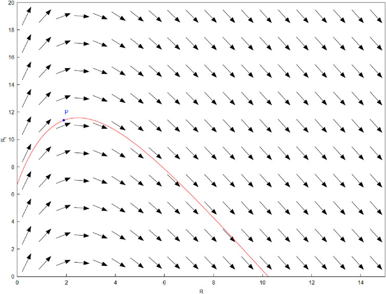
Figure 1. The dynamic system for the r-variable, Equation 28. Parameter values – $g=2.0$, $R_e=3.45$; drawn a trajectory passing through $P(1.9,11.4)$.

5 Properties of the state equations

To simplify presentation we further re-scale both time and population variables as

$\rho ≔r/g,\sigma ≔s/g,\iota ≔i/g,\tau ≔gt$

and differentiation with respect to $\tau$ will be denoted by a dot. Therefore, the equations of state Equation 30 acquire a very simple form

$\sigma =R_e{e}^{-\rho },(31)$

$\iota =R_e\left(1-e^{-\rho }\right)-\rho =\dot{\rho },(32)$

where Equation 30 follow from Equation 31, while Equation 32 follows from the construction of SIR model – i.e. the number conservation first integral. Therefore, at positive infinity $(\tau =+\infty )$ and for $R_e>1$ we have the triple

${\iota }_{\infty }=0,{\rho }_{\infty }=R_e+W_{+}\left(-R_e{e}^{-R_e}\right),{\sigma }_{\infty }=-W_{+}\left(-R_e{e}^{-R_e}\right)$

so that

$e^{-{\rho }_{\infty }}=-e^{-R_e}\frac{e^{R_e}{W}_{+}\left(-R_e{e}^{-R_e}\right)}{R_e}=-\frac{W_{+}\left(-R_e{e}^{-R_e}\right)}{R_e}(33)$

by Equation 5. While for $R_e>1$ and $\tau =-\infty$ it follows that

${\iota }_{-\infty }=0,{\rho }_{-\infty }=R_e+W_{-}\left(-R_e{e}^{-R_e}\right)=0,{\sigma }_{-\infty }=-W_{-}\left(-R_e{e}^{-R_e}\right)=R_e$

hold. These are limiting behaviors which should hold for any approximation of practical interest.

Furthermore, the outbreak peak is given by the triple:

${\iota }_m=R_e-1-\log R_e,{\rho }_m=\log R_e,{\sigma }_m=1,$

under the obvious conditions ${\iota }_m>0$, ${\rho }_m>0$, which is equivalent to $R_e>1$. Alternatively, the $R_e$ can be inferred from $i_m$ since

$R_e=-W_{-}\left(-e^{-{\iota }_m-1}\right)(34)$

Furthermore, the $\rho$ variable can be obtained explicitly as follows. We set $\rho =-\log y$ to obtain

$\iota =\log y-R_{e}y+R_e$

This equation is solvable with the help of the Lambert’s W function as

$y=-\frac{W_{\pm }\left(-R_e{e}^{\iota -R_e}\right)}{R_e}$

Therefore,

$\begin{array}{l}\hfill \rho =-\log \left(-\frac{W_{\pm }\left(-R_e{e}^{\iota -R_e}\right)}{R_e}\right)=\log R_e+R_e-\iota -\log R_e+W_{\pm }\left(-R_e{e}^{\iota -R_e}\right)=\\ \hfill R_e-\iota +W_{\pm }\left(-e^{\iota -{\iota }_m-1}\right)\end{array}(35)$

where the principal branch is taken for $\tau <0$ and the non-principal one – for $\tau >0$, respectively. In summary from Equations 33–35, in terms of the $\iota$ variable we obtain the equations

$\sigma =-W_{\pm }\left(-e^{\iota -{\iota }_m-1}\right)(36)$

$\rho =W_{\pm }\left(-e^{\iota -{\iota }_m-1}\right)-W_{-}\left(-e^{-{\iota }_m-1}\right)-\iota (37)$

in accordance with the first integral. The last Equations 36, 37 can be expressed concisely by the $\mathrm{\Omega }$ function as

$\sigma =-{\mathrm{\Omega }}_{\pm }\left(\iota -{\iota }_m-1\right)(38)$

$\rho ={\mathrm{\Omega }}_{\pm }\left(\iota -{\iota }_m-1\right)-{\mathrm{\Omega }}_{-}\left(-{\iota }_m-1\right)-\iota =-\sigma +R_e-\iota (39)$

with a similar convention for the branches.

6 Exponential series solution

6.1 Predictive series

First, we will look for a solution, approximating the r-variable on the positive real line. The asymptotic analysis indicates that an approximation may be achievable using a general Dirichlet series of the form:

$\rho -{\rho }_{\infty }={\displaystyle \sum _{k=1}^{\infty }}\frac{c_k{e}^{-km\tau }}{k!},\tau \ge 0(40)$

where $m$ is a real-valued exponent to be determined later. The truncation of the series at a finite $k$ is then a Prony series. Since we will characterize a dynamical system the Prony series will have exact instead of empirical character. Furthermore, since we are interested only in a Prony approximation we will treat the Equation 40 as formal series without regard to convergence issues.

The formal exponent of the Dirichlet series is another general Dirichlet series

$e^{{\rho }_{\infty }-\rho }=1+{\displaystyle \sum _{k=1}^{\infty }}\frac{{\left(-1\right)}^k{B}_k{e}^{-km\tau }}{k!}$

where the coefficients $B_k$ are given by the complete, exponential Bell polynomials $B_k\equiv B_k(c_1,\dots ,c_k)$.

The complete Bell polynomials in turn can be readily calculated from the determinant

$B_k\left(c_1,\dots ,c_k\right)=\left|\begin{array}{ccccc}\hfill \left(\begin{array}{c}k-1\\ 1\end{array}\right)c_1\hfill & \hfill \left(\begin{array}{c}k-1\\ 2\end{array}\right)c_2\hfill & \hfill \left(\begin{array}{c}k-1\\ 3\end{array}\right)c_3\hfill & \hfill \dots \hfill & \hfill c_k\hfill \\ \hfill -1\hfill & \hfill \left(\begin{array}{c}k-2\\ 1\end{array}\right)c_1\hfill & \hfill \left(\begin{array}{c}k-2\\ 2\end{array}\right)c_2\hfill & \hfill \dots \hfill & \hfill c_{n-1}\hfill \\ \hfill 0\hfill & \hfill -1\hfill & \hfill \left(\begin{array}{c}k-3\\ 1\end{array}\right)c_1\hfill & \hfill \dots \hfill & \hfill c_{k-2}\hfill \\ \hfill 0\hfill & \hfill 0\hfill & \hfill -1\hfill & \hfill \dots \hfill & \hfill c_{k-3}\hfill \\ \hfill \dots \hfill & \hfill \dots \hfill & \hfill \dots \hfill & \hfill \dots \hfill & \hfill \dots \hfill \\ \hfill 0\hfill & \hfill 0\hfill & \hfill 0\hfill & \hfill -1\hfill & \hfill c_1\hfill \end{array}\right|$

The first few polynomials can be listed as

$\begin{array}{l}\hfill B_0=0,B_1=c_1,B_2=c_2+c_1^2,B_3=c_3+3c_1{c}_2+c_1^3,\\ \hfill B_4=c_4+4c_1{c}_3+3c_2^2+6c_1^2{c}_2+c_1^4,B_5=c_5+5c_1{c}_4+10c_2{c}_3+10c_1^2{c}_3+15c_1{c}_2^2+10c_1^3{c}_2+c_1^5,\dots \end{array}$

We substitute the above expressions in Equation 27, which obtains the form

$\ddot{\rho }=\dot{\rho }\left(R_e{e}^{-\rho }-1\right)$

Observe that reversing time direction will result in a change of sign of the right-hand side of the equation. Therefore, it will be sufficient to determine the coefficients only for the positive time direction. The resulting expression is

$m^2{\displaystyle \sum _{k=1}^{\infty }}{k}^2\frac{c_k{e}^{-km\tau }}{k!}=-m\left({\displaystyle \sum _{k=1}^{\infty }}k\frac{c_k{e}^{-km\tau }}{k!}\right)\left(R_e{e}^{-{\rho }_{\infty }}-1+R_e{e}^{-{\rho }_{\infty }}{\displaystyle \sum _{k=1}^{\infty }}\frac{{\left(-1\right)}^k{B}_k{e}^{-km\tau }}{k!}\right)$

Since we work with formal infinite series one can apply the Cauchy product formula. Therefore, we obtain the equation

$\begin{array}{l}\hfill R_{e}m{\displaystyle \sum _{k=1}^{\infty }}\frac{k{c}_k{e}^{-{\rho }_{\infty }-km\tau }}{k!}+R_{e}m{e}^{-{\rho }_{\infty }}{\displaystyle \sum _{k=2}^{\infty }}{\displaystyle \sum _{i=1}^{k-1}}\frac{{\left(-1\right)}^i{B}_i\left(k-i\right)c_{k-i}{e}^{-km\tau }}{i!\left(k-i\right)!}+\\ \hfill m^2{\displaystyle \sum _{k=1}^{\infty }}\frac{k^2{c}_k{e}^{-km\tau }}{k!}-m{\displaystyle \sum _{k=1}^{\infty }}\frac{k{c}_k{e}^{-km\tau }}{k!}=0\end{array}$

Equating the exponents results in the following recursion dependence between the coefficients:

$k^2{c}_{k}m{e}^{{\rho }_{\infty }}-k{c}_k{e}^{{\rho }_{\infty }}+R_e{\displaystyle \sum _{i=1}^k}k!\frac{{\left(-1\right)}^i{B}_i{c}_{k-i}}{i!\left(k-i-1\right)!}+R_{e}k{c}_k=0(41)$

The first terms of the recursion are

$\begin{array}{l}\hfill \left\{0,c_1\left(e^{{\rho }_{\infty }}m-e^{{\rho }_{\infty }}+R_e\right),2\left(2c_2{e}^{{\rho }_{\infty }}m-c_2{e}^{{\rho }_{\infty }}+c_2{R}_e-c_1^2{R}_e\right),\right.\\ \hfill \left.3\left(3c_3{e}^{{\rho }_{\infty }}m-c_3{e}^{{\rho }_{\infty }}+c_3{R}_e-c_1{c}_2{R}_e+c_1^3{R}_e\right),\dots \right\}\end{array}$

Therefore, for the base exponent $m=1-R_e{e}^{-{\rho }_{\infty }}=1+W_{+}\left(-R_e{e}^{-R_e}\right)$ must hold as a constraint for a non trivial series solution to exist. By using the value of $m$ found in this way $c_k$ can be obtained by recursion from Equation 41:

$c_k=-\frac{q}{k-1}{\displaystyle \sum _{i=1}^k}{\left(-1\right)}^i\left(\genfrac{}{}{0.0pt}{}{k-1}{i}\right)B_i{c}_{k-i},k\ge 2$

where we have recognized the appearance of the Newton’s binomial coefficients and

$q=\frac{R_e}{e^{{\rho }_{\infty }}-R_e}=\frac{-W_{+}\left(-R_e{e}^{-R_e}\right)}{1+W_{+}\left(-R_e{e}^{-R_e}\right)}$

The first few coefficients of the series can be readily computed as

$\begin{array}{l}\hfill c_1=\lambda ,c_2=-q{\lambda }^2,c_3=\frac{q\left(q+1\right){\lambda }^3}{2},c_4=\frac{q\left(q^2-2q-1\right){\lambda }^4}{3},\\ \hfill c_5=-\frac{q\left(q-1\right)\left(2q^2+5q+1\right){\lambda }^5}{4},c_6=-\frac{q\left(27q^4-37q^3-49q^2+49q+6\right){\lambda }^6}{30},\\ \hfill c_7=\frac{q\left(98q^5+311q^4-295q^3-227q^2+197q+12\right){\lambda }^7}{72},\dots \end{array}$

Substituting the value of q produces an equivalent form of the sequence as

$\begin{array}{l}\hfill c_2=\frac{c_1^2{R}_e}{e^{{\rho }_{\infty }}-R_e},c_3=-\frac{c_1^3{R}_e\left(e^{{\rho }_{\infty }}-2R_e\right)}{2{\left(e^{{\rho }_{\infty }}-R_e\right)}^2},c_4=\frac{c_1^4{R}_e\left(e^{2{\rho }_{\infty }}-4R_e{e}^{{\rho }_{\infty }}+2{R_e}^2\right)}{3{\left(e^{{\rho }_{\infty }}-R_e\right)}^3},\\ \hfill c_5=-\frac{c_1^5{R}_e{e}^{{\rho }_{\infty }}\left(e^{2{\rho }_{\infty }}-7R_e{e}^{{\rho }_{\infty }}+8{R_e}^2\right)}{4{\left(e^{{\rho }_{\infty }}-R_e\right)}^4},\dots \end{array}$

The above procedure is essentially algorithmic and easily amenable to programming in a computer algebra system. The procedure leaves the coefficient $c_1=\lambda$ undetermined. Therefore, the result is a combined series in $\tau$ and $\lambda$:

$\rho \left(\tau |\lambda \right)={\rho }_{\infty }+{\displaystyle \sum _{k=1}^{\infty }}\frac{c_k{\lambda }^k{e}^{-km\tau }}{k!},\tau \ge 0$

where now $c_k$ are appropriately re-scaled from $c_1=1$. This amounts to a time-sift of the origin with $\log \lambda /m$ since

$\rho \left(\tau |\lambda \right)={\rho }_{\infty }+{\displaystyle \sum _{k=1}^{\infty }}\frac{c_k{e}^{-k\left(m\tau -\log \lambda \right)}}{k!},\tau \ge 0,\lambda \ne 0$

Furthermore, observe that $\lambda =0$ corresponds to the positive infinity, since then $\rho (\tau |0)={\rho }_{\infty }$.

6.2 Retrodictive series

In this section we revert the time direction and look for series of the form

$\rho ={\displaystyle \sum _{k=1}^{\infty }}\frac{c_k{e}^{km\tau }}{k!},\tau <0$

which asymptotically approaches ${\rho }_{-\infty }=0$. The first terms of the recursion are

$\begin{array}{l}\hfill \left\{0,c_1\left(m-R_e+1\right),2\left(2c_{2}m-c_2{R}_e+B_1{c}_1{R}_e+c_2\right),3\left(3c_{3}m-c_3{R}_e+2B_1{c}_2{R}_e-c_1{B}_2{R}_e+c_3\right)\right.,\\ \hfill \left.4,\left(4c_{4}m-c_4{R}_e+3B_1{c}_3{R}_e+c_1{B}_3{R}_e-3B_2{c}_2{R}_e+c_4\right),,,\dots \right\}\end{array}$

Therefore, $m=R_e-1$. The same kind of analysis leads to the recursion

$k^2{c}_{k}m-R_{e}k!\left({\displaystyle \sum _{i=1}^{k-1}}\frac{{\left(-1\right)}^i{B}_i\left(k-i\right)c_{k-i}}{i!\left(k-i\right)!}\right)-R_{e}k{c}_k+k{c}_k=0$

Therefore,

$c_k=\frac{R_e}{\left(R_e-1\right)\left(k-1\right)}{\displaystyle \sum _{i=1}^k}{\left(-1\right)}^i\left(\genfrac{}{}{0.0pt}{}{k-1}{i}\right)B_i{c}_{k-i},k\ge 2$

This results in coefficients

$\begin{array}{l}\hfill c_2=\frac{c_1^2{R}_e}{R_e-1},c_3=-\frac{c_1^3{R}_e\left(2R_e-1\right)}{2{\left(R_e-1\right)}^2},c_4=\frac{c_1^4{R}_e\left(2{R_e}^2-4R_e+1\right)}{3{\left(R_e-1\right)}^3},\\ \hfill c_5=-\frac{c_1^5{R}_e\left(8{R_e}^2-7R_e+1\right)}{4{\left(R_e-1\right)}^4},c_6=\frac{c_1^6{R}_e\left(4{R_e}^4+36{R_e}^3-134{R_e}^2+73R_e-6\right)}{30{\left(R_e-1\right)}^5},\dots \end{array}$

Therefore, as before we can set $c_1=\lambda$ and obtain the series

$\rho \left(\tau |\lambda \right)={\displaystyle \sum _{k=1}^{\infty }}\frac{c_k{\lambda }^k{e}^{km\tau }}{k!},\tau <0$

In summary, as before we can determine the solution up to translation in time.

6.3 Peak value parametrization - predictive series

In this section, we use the peak parametrization where ${\rho }_0={\rho }_m=\log R_e$ and form the infinite series

$\rho -{\rho }_0≔{\displaystyle \sum _{k=1}^{\infty }}\frac{c_k\left(1-e^{-km\tau }\right)}{k!}=A-{\displaystyle \sum _{k=1}^{\infty }}\frac{c_k{e}^{-km\tau }}{k!},t\ge 0$

where we also denote the infinite sum $A≔{\sum }_{k=1}^{\infty }{c}_k/k!$. Then, at positive infinity, the value of $A$ can be determined as

${\rho }_{\infty }-{\rho }_0=R_e+W_{+}\left(-R_e{e}^{-R_e}\right)-\log R_e=A\ge 0$

The Lambert function identity $W_{+}\left(-1/e\right)=-1$ shows that $R_e=1$ implies $A=0$.

The same development procedure produces the recursion

$c_k=-\frac{q}{k-1}{\displaystyle \sum _{i=1}^k}{\left(-1\right)}^i\left(\begin{array}{c}\hfill k-1\hfill \\ \hfill i\hfill \end{array}\right)B_i{c}_{k-i},k\ge 2(42)$

where now

$q=\frac{1}{e^A-1}$

The coefficients are still given by Equation 42 but expressed in terms of A can be read off as

$\begin{array}{l}\hfill c_1=\lambda ,c_2=\frac{{\lambda }^2}{e^A-1},c_3=-\frac{{\lambda }^3\left(e^A-2\right)}{2{\left(e^A-1\right)}^2},c_4=\frac{{\lambda }^4\left(e^{2A}-4e^A+2\right)}{3{\left(e^A-1\right)}^3},\\ \hfill c_5=-\frac{{\lambda }^5{e}^A\left(e^{2A}-7e^A+8\right)}{4{\left(e^A-1\right)}^4},c_6=\frac{{\lambda }^6\left(6e^{4A}-73e^{3A}+134e^{2A}-36e^A-4\right)}{30{\left(e^A-1\right)}^5},\dots \end{array}$

while the base exponent is $m=1-e^{-A}$.

6.4 Peak value parametrization – retrodictive series

We start from the equation

$\rho -{\rho }_0≔-A+{\displaystyle \sum _{k=1}^{\infty }}\frac{c_k{e}^{km\tau }}{k!},\tau <0(43)$

where ${\rho }_0=\log R_e$. Then asymptotically

${\rho }_{-\infty }-\log R_e=-A\Rightarrow A=\log R_e$

So it follows that

$\rho ={\displaystyle \sum _{k=1}^{\infty }}\frac{c_k{e}^{km\tau }}{k!}$

${\displaystyle \sum _{k=1}^{\infty }}\frac{{\lambda }^k{c}_k}{k!}=\log R_e$

where $m=R_e-1$, $q=R_e/(R_e-1)$, and $c_1=\lambda$.

In summary, the presented approach is manifestly time-asymmetric due to the properties of the equivalent dynamical system for the r-variable.

6.5 The i-variable

The other observable of the model is the $\iota$ variable, which can be obtained from Equation 32:

$\iota \left(\tau \right)=R_e-\sigma \left(\tau \right)-\rho \left(\tau \right)=R_e\left(1-\exp \left(-\rho \left(\tau \right)\right)\right)-\rho \left(\tau \right)$

Therefore, by substitution

$\iota \left(\tau \right)=R_e\left(1-\exp \left(-\left({\rho }_0+A\right)+{\displaystyle \sum _{k=1}^{\infty }}\frac{c_k{e}^{-km\tau }}{k!}\right)\right)-\left({\rho }_0+A\right)+{\displaystyle \sum _{k=1}^{\infty }}\frac{c_k{e}^{-km\tau }}{k!}$

For the value at $\tau =0$ one obtains

$\iota \left(0\right)=R_e\left(1-\exp \left(-{\rho }_0\right)\right)-{\rho }_0=R_e-1-\log R_e={\iota }_m$

and finally

$\iota \left(\tau \right)=R_e\left(1-e^{-{\rho }_{\infty }}\exp \left({\displaystyle \sum _{k=1}^{\infty }}\frac{c_k{e}^{-km\tau }}{k!}\right)\right)-{\rho }_{\infty }+{\displaystyle \sum _{k=1}^{\infty }}\frac{c_k{e}^{-km\tau }}{k!},\tau \ge 0$

For the case $\tau <0$ we proceed in a similar way.

$\iota \left(\tau \right)=R_e\left(1-\exp \left(-{\displaystyle \sum _{k=1}^{\infty }}\frac{c_k{e}^{km\tau }}{k!}\right)\right)+{\displaystyle \sum _{k=1}^{\infty }}\frac{c_k{e}^{km\tau }}{k!},\tau <0$

Then

$\iota \left(0\right)=R_e\left(1-e^{-\log R_e}\right)-\log R_e={\iota }_m$

so that the series agree.

The asymptotes at infinity are verified by direct substitution

$\iota \left(\pm \infty \right)=R_e\left(1+\frac{W_{\pm }\left(-R_e{e}^{-R_e}\right)}{R_e}\right)-\left(R_e+W_{\pm }\left(-R_e{e}^{-R_e}\right)\right)=0$

6.6 The s-variable

The series for the s-variable can be determined from the state equations as

$\sigma \left(\tau \right)=R_e\exp \left(-\rho \left(\tau \right)\right)=R_e{e}^{-{\rho }_{\infty }}\exp \left({\displaystyle \sum _{k=1}^{\infty }}\frac{c_k{e}^{-km\tau }}{k!}\right),\tau \ge 0$

and

$\sigma \left(\tau \right)=R_e\exp \left(-{\displaystyle \sum _{k=1}^{\infty }}\frac{c_k{e}^{km\tau }}{k!}\right),\tau <0$

7 Non-linear approximation procedure

Since the SIR solution is non-singular everywhere in $\mathbb{R}$, one can apply the Banach Fixed-Point Theorem to obtain non-linear approximation. Notably, one can use the non-linear approximation scheme of Daftardar-Gejji-Jafari (DJM method) for solving the equivalent integral Equation 16 [17].

7.1 The double-exponential approximate solution

Starting from the 0^th order approximation $i^{(0)}\approx i_0$, it follows that $s^{(0)}\approx s_0{e}^{-i_0\tau }$. However, this does not guarantee convergence of the iteration. To establish convergence we observe that $s=g$ is a fixed point of Equation 22 since $di/ds=0$ for this point and, therefore, the Banach theorem can be applied. Therefore, we must take $s_0=g$ as an initial condition. This corresponds to the peak-value parameterization so that $i_0=i_m$, $i^{\prime }(0)=0$ and by Equation 27:

$i\left(\tau \right)=i_m\exp \left(g{\int }_0^{\tau }{e}^{-{\int }_0^{z}i\left(y\right)dy}dz-g\tau \right)$

can be formulated as a functional integral equation to be approximated by DJM.

From there the first order approximation for the i-variable becomes the double exponential function

$i^{\left(1\right)}=i_m{e}^{\frac{g}{i_m}\left(1-e^{-i_{m}t}\right)-gt}(44)$

The corresponding solution for $r$ will be

$r^{\left(1\right)}=R_{e}g-i^{\left(1\right)}+g{W}_{\pm }\left(-R_e{e}^{\frac{i^{\left(1\right)}}{g}-R_e}\right)(45)$

where we take the non-principal branch $W_{-}$ for $t<0$ and the principal one $W_{+}$ for $t>0$. The s-variable can be expressed accordingly

$s^{\left(1\right)}=-g{W}_{\pm }\left(-R_e{e}^{\frac{i^{\left(1\right)}}{g}-R_e}\right)(46)$

Therefore, we can claim:

Proposition 4. The double-exponential, approximate analytic solution of the SIR model is given by Equations 44–46.

The advantage of this formulation is that it respects the population size integral as well as the fixed points of the dynamical system.

On the other hand, formulated through the $\rho$ variable, the integral equation

$\rho \left(\tau \right)={\iota }_m{\int }_0^{\tau }\exp \left(R_e{\int }_0^y{e}^{-\rho \left(z\right)}dz-y\right)dy+\log R_e$

also holds. However, iterating this system will not lead to global convergence towards the analytical solution since $\rho =\log R_e$ is not a fixed point but an inflection point for $\rho$. A similar argument can be brought forward also for the $s$-variable. Therefore, one must use Equations 45, 46 to obtain the approximate analytic solutions.

To link this approach with the Prony approximation one observes that

$i^{\left(1\right)}=i_m{e}^{\frac{g}{i_m}-gt}{e}^{-\frac{g}{i_m}{e}^{-i_{m}t}}=i_m{e}^{\frac{g}{i_m}-gt}{\displaystyle \sum _{k=0}^{\infty }}\frac{1}{k!}{\left(\frac{-g}{i_m}\right)}^k{e}^{-k{i}_{m}t}$

which has the form of a general Dirichlet series and can be readily truncated into Prony approximation. From this analysis one can interpret $i_m$ as a timescale rather than an amplitude parameter. This is a useful interpretation also for the numerical fitting procedure as there the population size N can be treated as an additional degree of freedom.

7.2 The $\mathrm{\Gamma }$-approximate solution

DJM method can be further applied as follows. The second iteration of the DJM method results in a $\mathrm{\Gamma }$-integral:

$\begin{array}{l}\hfill J=\int e^{\frac{g}{i_m}\left(1-e^{-i_m\tau }\right)-g\tau }d\tau ={\left.-\int y^{\frac{g}{i_m}-1}{e}^{\frac{g}{i_m}-\frac{gy}{i_m}}dy\right|}_{y=e^{-i_m\tau }}=\\ \hfill -\frac{\mathrm{\Gamma }\left(\frac{g}{i_m},\frac{g}{i_m}{e}^{-i_m\tau }\right)}{{\left(\frac{g}{i_m}\right)}^{\frac{g}{i_m}}}{e}^{\frac{g}{i_m}}=-\frac{e^a}{a^a}\mathrm{\Gamma }\left(a,a{e}^{-i_m\tau }\right),a=g/i_m\end{array}$

where $\mathrm{\Gamma }(a,x)$ is the upper incomplete Euler’s gamma function. Following the same procedure for the i-variable we obtain

$i^{\left(2\right)}=i_m\exp \left(g{\int }_0^{\tau }{e}^{q\left(\mathrm{\Gamma }\left(a,a\right)-\mathrm{\Gamma }\left(a,a{e}^{-i_{m}z}\right)\right)}dz-g\tau \right),q={\left(\frac{e}{a}\right)}^a(47)$

This is another non-elementary integral which can be readily computed by quadratures as it involves one of the common special functions.

8 Newtonian approximation of the r-variable

The R-variable can be computed by numerical inversion of Equation 19. A suitable algorithm to do so is the Newton-Raphson approximation based on the double-exponential formula. An approximation schema can be derived for an input $(t,g,i_m)$ and initialization parameters

$\begin{array}{ll}\hfill I& =i_m{e}^{g\left(1-e^{-i_{m}t}\right)/i_m-gt}\hfill \\ \hfill N& =-g{W}_{-}\left(-e^{-i_m/g-1}\right)\hfill \\ \hfill \mathrm{\Delta }& =N-i_m-g=g\log N\hfill \end{array}$

Let

$F\left(r\right)≔t-\frac{1}{g}\underset{r}{\overset{\mathrm{\Delta }}{\int }}\frac{dy}{N\left(e^{-y/g}-1\right)+y}$

Then the iteration schema is

$r_{n+1}=r_n-\frac{F\left(r_n\right)}{F^{\prime }\left(r_n\right)}$

Therefore,

$r_0=N-I+g{W}_{\pm }\left(\left(I-i_m\right)/g-1\right)$

$r_{n+1}=r_n-\left(N\left(e^{-r_n/g}-1\right)+r_n\right)F\left(r_n\right)$

where we take the non-principal branch $W_{-}$ for $t<0$ and the principal one $W_{+}$ for $t>0$. The advantage of the above formulation is that the integral kernel is elementary and the Lambert W function is evaluated only during the initialization of the algorithm. The schema converges wherever the quantity

$M≔\left|\frac{F^{\prime \prime }}{2F^{\prime }}\right|=\left|\frac{1-R_e{e}^{-r/g}}{2g\left(R_e\left(e^{-r/g}-1\right)+r/g\right)}\right|$

is bounded–that is, wherever the initial value $r_0$ is sufficiently far from the poles of the kernel, which are the zeroes of the denominator, given by Equation 21: $r_{\mathrm{1,2}}=g{y}_{\mathrm{1,2}}$. Observe that the denominator has an extremum at $r_m=g\log R_e$. Therefore, we can investigate the convergence in the two intervals $(0,r_m)$ and $[r_m,g{y}_1)$. Suppose that $r/g=ϵ$ could be thought of as infinitesimal quantity. Then to first order in $ϵ$

$Mϵ\approx ϵ\left|\frac{1-R_e\left(1-ϵ\right)}{2gϵ\left(1-R_e\right)}\right|=\left|\frac{1-R_e\left(1-ϵ\right)}{2g\left(1-R_e\right)}\right|=\frac{1}{2g}\left|1+\frac{R_eϵ}{1-R_e}\right|<\frac{1}{2g}$

since $R_e>1$. Therefore, for $r_0\ge 2gϵ$ the method will converge.

Furthermore, suppose that the value of the denominator $R_e(e^{-r/g}-1)+r/g=ϵ$ could be thought of as infinitesimal quantity. Then to first order in $ϵ$

$\begin{array}{l}\hfill Mϵ=\frac{1}{2g}\left|1-R_e{e}^{-r/g}\right|\approx \frac{1}{2g}\left|1-\left(ϵ-r/g+R_e\right)\right|<\frac{1}{2g}\left|1+r/g-R_e\right|=\\ \hfill \frac{1}{2g}\left|1+W_{+}\left(-R_e{e}^{-R_e}\right)\right|<\frac{1}{2g}\end{array}$

since $W_{+}\left(-R_e{e}^{-R_e}\right)<0$. Therefore, for $g{y}_1-r_0\ge 2gϵ$ the method will converge. Therefore, the schema has the desired quadratic convergence whenever M is bounded.

Validation data on the approach are included in the Supplementary Material.

9 Numerical results

The asymptotics of the i-variable are compared with the parametric solution in Figure 2. Figure 3 demonstrates the approximate double-exponential SIR model. The parametric solution for the $r$-variable is compared with the 3-term Prony series in Figure 4. Plots of the parametric solution were obtained by direct numerical integration using the QUADPACK [18] routines in the Computer Algebra System Maxima. Figure 5 compares the parametric solution for the r-variable with the double-exponential approximate solution. The approximate solution shows global convergence to the parametric one as expected.

Figure 2

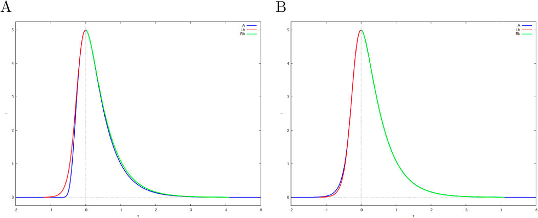
Figure 2. Parametric and asymptotic solutions for the incidence variable $i(\tau )$. Asymptotic solutions compared to parametric plots of $(\tau (i),i)$ parameterized by $i_m=5.0$ and $g=2.0$. Legends: Lb denotes the left branch using $W_{-}(x)$, Rb denotes the right branch using $W_{+}(x)$, Equation 18. A denotes the asymptotic solution. (A) the double exponential asymptotic for $i(\tau )$ is computed from Equation 44; (B) the gamma-asymptotic for $i(\tau )$ is computed from Equation 47. Plots were produced using the quad_qags Maxima numerical integration command.

Figure 3

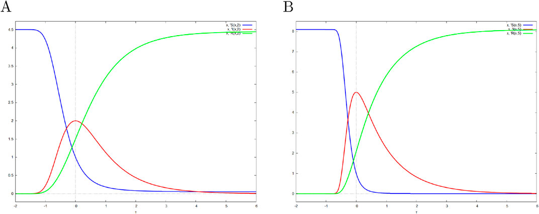
Figure 3. Double-exponential approximation of the SIR model. S, I, R denote the s(t), i(t) and r(t) first order approximations, respectively. (A) $i_m=2$; (B) $i_m=5$.

Figure 4

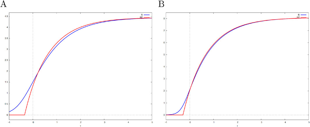
Figure 4. 3-term Prony predictive approximation of the r-variable. ilambint61 denotes the parametric solution, R3 denotes 3-term Prony approximation. (A) $i_m=2$; (B) $i_m=5$. Numerical experiments indicate that $\lambda \approx A$ (Equation 43) provides a good fit.

Figure 5

Figure 5. Approximation of the r-variable. R denotes the parametric solution, R1 denotes the approximate solution, given by Equation 45. (A) $i_m=2$; (B) $i_m=5$.

10 A case study in epidemiology

The approach was applied to the boarding school flu dataset. The influenza data are tabulated in [2]. The table is reproduced as a Supplementary Material. The parametric fitting was conducted using a least-squares constrained optimization algorithm. The least-squares constrained optimization was preformed using the fminsearchbnd routine [19]. The fitting equations are given by

$R\sim N{r}^{\left(1\right)}\left(t-T|g,i_m\right)$

for the observed cumulative incidence $R$, as a proxy for the recovered population, and

$I\sim N{i}^{\left(1\right)}\left(t-T|g,i_m\right)$

where $I$ is the observed incidence. The parameter estimation procedure is demonstrated in the Supplementary Material. The results of the procedure are reported in Table 1. The peak could be correctly estimated as 296 cases. Variables are plotted in Figure 6. The fitted curves match closely the raw data. Both estimation procedures agree well on the value of the excitation timescale $i_m$, while they differ for the relaxation timescale g.

Table 1

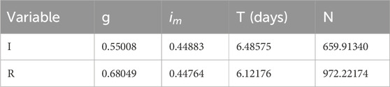
Table 1. Estimated SIR model parameters.

Figure 6

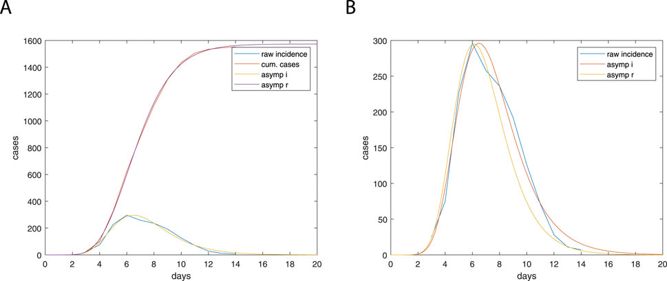
Figure 6. Asymptotic fitting of reported cases. (A) Comparison between the raw data and fitted curves for the infected (“asymp i”) and recovered populations (“asymp r”); (B) Incidence data compared to fitted curves. Parameters from Table 1 were used to compute the incidence curves, “asymp i” – fitting for I, “asymp r” – fitting for R.

11 Discussion and conclusion

The contributions of the present article are three fold. On the first place, the article presents an infinite exponential series solutions, converging on the real half-plane. The presented exponential series explicitly characterizes the non-elementary $r$-variable and by virtue of the state equations also the $s$- and $i$-variables of the SIR model. Furthermore, the present paper expands the utility of Prony series approximation towards mathematical epidemiology. The recovery can be transparently represented as a series of relaxation processes having different time constants, which could improve our conceptual understanding of the emergence of different time scales in epidemiological models. This is a phenomenon also captured by the double-exponential, Gompertzian, solution [20] where the fast time-scale emerges from the global property of the system – that is the population size through the excitation timescale $i_m$. The presence of such a phenomenon is not apparent from the form of the differential equations only, as these explicate only the longer time scale $g$. In such way, the appearance of the faster time scale is a truly emergent phenomenon.

The time-asymmetry of the dynamical system for the R-variable dictates the appearance of the very different forms of the exponential series. Most likely this phenomenon will hold also in other models derived from SIR, such as SEIR and SIRD.

On the second place, a new numerical approximation schema was derived for the R-variable. To obtain convergence to the correct branch it is crucial to start from an initial approximation, which is close to the exact solution.

Finally, the non-linear approximation produces produces and approximate analytic solution which matches globally the previously-obtained parametric solution of the SIR system. The global solutions are represented as compositions of Lambert W function with elementary ones, which furthers the utility of the Lambert W and the closely related $\mathrm{\Omega }$ function for applied mathematical applications. This can be used for data-fitting purposes and can become a widely used predictive tool for epidemic outbreak control.

Data availability statement

The original contributions presented in the study are included in the article/Supplementary Material, further inquiries can be directed to the corresponding author.

Author contributions

DP: Writing–original draft, Writing–review and editing.

Funding

The author(s) declare that no financial support was received for the research, authorship, and/or publication of this article.

Conflict of interest

Author DP was employed by IMEC.

Publisher’s note

All claims expressed in this article are solely those of the authors and do not necessarily represent those of their affiliated organizations, or those of the publisher, the editors and the reviewers. Any product that may be evaluated in this article, or claim that may be made by its manufacturer, is not guaranteed or endorsed by the publisher.

Supplementary material

The Supplementary Material for this article can be found online at: https://www.frontiersin.org/articles/10.3389/fphy.2024.1469663/full#supplementary-material

References

1. Kermack WO, McKendrick AG. A contribution to the mathematical theory of epidemics. Proc R Soc Lond Ser A, Containing Pap a Math Phys Character (1927) 115:700–21. doi:10.1098/rspa.1927.0118

CrossRef Full Text | Google Scholar

2. Martcheva M. An introduction to mathematical epidemiology. Springer US (2015). doi:10.1007/978-1-4899-7612-3

CrossRef Full Text | Google Scholar

3. Hethcote HW. The mathematics of infectious diseases. SIAM Rev (2000) 42:599–653. doi:10.1137/s0036144500371907

CrossRef Full Text | Google Scholar

4. Tang L, Zhou Y, Wang L, Purkayastha S, Zhang L, He J, et al. A review of multi-compartment infectious disease models. International Statistical Review 88 (2020) 462–513. doi:10.1111/insr.12402

PubMed Abstract | CrossRef Full Text | Google Scholar

5. Funk S, Gilad E, Watkins C, Jansen VAA. The spread of awareness and its impact on epidemic outbreaks. Proc Natl Acad Sci (2009) 106:6872–7. doi:10.1073/pnas.0810762106

PubMed Abstract | CrossRef Full Text | Google Scholar

6. Kendall D. Deterministic and stochastic epidemics in closed populations. Berkeley Symp Math Stat Probab (1956) 4:149–65. doi:10.1525/9780520350717-011

CrossRef Full Text | Google Scholar

7. Harko T, Lobo FSN, Mak MK. Exact analytical solutions of the susceptible-infected-recovered (SIR) epidemic model and of the SIR model with equal death and birth rates. Appl Mathematics Comput (2014) 236:184–94. doi:10.1016/j.amc.2014.03.030

CrossRef Full Text | Google Scholar

8. Barlow NS, Weinstein SJ. Accurate closed-form solution of the SIR epidemic model. Physica D: Nonlinear Phenomena (2020) 408:132540. doi:10.1016/j.physd.2020.132540

PubMed Abstract | CrossRef Full Text | Google Scholar

9. Kröger M, Schlickeiser R. Analytical solution of the SIR-model for the temporal evolution of epidemics. Part A: time-independent reproduction factor. J Phys A: Math Theor (2020) 53:505601. doi:10.1088/1751-8121/abc65d

CrossRef Full Text | Google Scholar

10. Prodanov D. Analytical parameter estimation of the SIR epidemic model. applications to the COVID-19 pandemic. Entropy (Basel, Switzerland) (2020) 23:59. doi:10.3390/e23010059

PubMed Abstract | CrossRef Full Text | Google Scholar

11. Prodanov D. Comments on some analytical and numerical aspects of the SIR model. Appl Math Model (2021) 95:236–43. doi:10.1016/j.apm.2021.02.004

CrossRef Full Text | Google Scholar

12. Kudryashov NA, Chmykhov MA, Vigdorowitsch M. Analytical features of the SIR model and their applications to COVID-19. Appl Math Model (2021) 90:466–73. doi:10.1016/j.apm.2020.08.057

PubMed Abstract | CrossRef Full Text | Google Scholar

13. Bougoffa L, Bougouffa S, Khanfer A. Approximate and parametric solutions to sir epidemic model. Axioms (2024) 13:201. doi:10.3390/axioms13030201

CrossRef Full Text | Google Scholar

14. Corless RM, Gonnet GH, Hare DEG, Jeffrey DJ, Knuth DE. On the Lambert W function. Adv Comput Mathematics (1996) 5:329–59. doi:10.1007/bf02124750

CrossRef Full Text | Google Scholar

15. Bronstein M, Corless RM, Davenport JH, Jeffrey DJ. Algebraic properties of the Lambert W function from a result of rosenlicht and of liouville. Integral Transforms Spec Functions (2008) 19:709–12. doi:10.1080/10652460802332342

CrossRef Full Text | Google Scholar

16. Corless RM, Jeffrey DJ. The Wright Omega function. In: Lecture notes in computer science. Berlin Heidelberg: Springer (2002). p. 76–89. doi:10.1007/3-540-45470-5_10

CrossRef Full Text | Google Scholar

17. Daftardar-Gejji V, Jafari H. An iterative method for solving nonlinear functional equations. J Math Anal Appl (2006) 316:753–63. doi:10.1016/j.jmaa.2005.05.009

CrossRef Full Text | Google Scholar

18. Piessens R, Doncker-Kapenga E, Überhuber CW, Kahaner DK. Quadpack. Springer Berlin Heidelberg (1983). doi:10.1007/978-3-642-61786-7

CrossRef Full Text | Google Scholar

19. [Dataset] Errico D. MATLAB Central Exchange (2012). Available from: https://www.mathworks.com/matlabcentral/fileexchange/8277-fminsearchbnd-fminsearchcon (Accessed July 29 2019).

20. Prodanov D. Computational aspects of the approximate analytic solutions of the sir model: applications to modelling of covid-19 outbreaks. Nonlinear Dyn (2023) 111:15613–31. doi:10.1007/s11071-023-08656-8

CrossRef Full Text | Google Scholar