Research on the prediction method of wing structure noise based on the combination of conditional generative adversarial neural network and numerical methods

This paper presents a technique for predicting noise generated by airfoil structures that combines deep learning techniques with traditional numerical methods. In traditional numerical methods, accurately predicting the noise of airfoil structures requires significant computational resources, making it challenging to perform low-noise optimization design for these structures. To expedite the prediction process, this study introduces Conditional Generative Adversarial Networks (CGAN). By replacing the generator and discriminator of CGAN with traditional regression neural network models, the suitability of CGAN for regression prediction is ensured. In this study, the data computation was accelerated by expanding the kernel function in the traditional boundary element method using a Taylor series. Based on the resulting data, an alternative predictive model for wing structure noise was developed by integrating Conditional Generative Adversarial Networks (CGAN). Finally, the effectiveness and feasibility of the proposed method are demonstrated through three case studies.

1 Introduction

The propeller is usually an open (non-enclosed) rotating mechanical device with multiple blades, and it has a history of nearly a century as an aviation propulsion system [1, 2]. As early as the 1940s, propellers were widely used in various types of aircraft, and the development of propeller technology has always been closely linked to the development of aircraft. Propeller engines are still widely used in military and civilian aircraft today, mainly due to their excellent fuel economy [3]. However, the propulsion speed of propellers significantly decreases under high subsonic conditions, resulting in relatively low cruising speeds for propeller-driven aircraft. Later, the concept of contra-rotating propeller engines was proposed. The contra-rotating propeller engine is a conceptually different aviation engine related to the turboprop engine and turbofan engine, and it is also referred to as a propeller fan engine, advanced turboprop engine, un ducted fan, or ultra-high bypass ratio turbofan engine [4, 5]. The design objective is to balance the efficiency and fuel economy of turboprop engines with the cruising speed and performance of turbofan engines [6–8], filling the speed gap between conventional turboprop engines and turbofan engines. It effectively addresses the contradiction between the cruising speed and propulsive efficiency of conventional turboprop engines and turbofan engines, and it is the direction of development for the propulsion systems of future medium-sized transport aircraft [9].

Compared to the 1980s, although modern contra-rotating propellers have made significant advances in aerodynamic design [10], noise optimization techniques, and manufacturing processes, according to NASA’s research, contra-rotating propeller engines still have a noise level that is more than 10 dB higher than that of ducted fan engines [11]. Therefore, aerodynamic and noise optimization design remains a key technical issue in the development of contra-rotating propellers [12]. However, due to the complex aerodynamic disturbances such as viscous wake interference, potential flow field interference, and propeller tip vortex interference between the two rows of propellers, the aerodynamic noise mechanism is more complicated [13–15]. Therefore, noise prediction and acoustic optimization design of propeller engines have become one of the key technologies in propeller design [16].

As the main component of propeller noise, accurate prediction of the noise generated by airfoils can guide the optimization design of propellers. Currently, in addition to using engineering estimation methods based on empirical theories, common methods for predicting airfoil vibration noise mainly rely on numerical calculation methods [17]. Engineering estimation methods typically use semi-theoretical and semi-empirical formulas combined with structural sound radiation theory and measured data. Engineering estimation methods are convenient and fast, but they are mainly applicable to specific structures or their similar models. Numerical simulation methods mainly rely on finite element methods (FEM) [18], boundary element methods (BEM) [19–21], and computational aeroacoustic methods (CAA) [22]. Among them, CAA methods combine computational fluid dynamics (CFD) simulations and the FW-H analogy method, which can simultaneously obtain the near-field flow distribution of the structure and the far-field acoustic characteristics, making it one of the reliable methods. However, in the pre-processing stage of CAA calculations, it is necessary to establish a very detailed model in the computer, which requires a significant amount of time and leads to a longer prediction process. Therefore, developing efficient aerodynamic noise prediction methods by combining deep learning methods can significantly reduce the computational cost of aerodynamic noise [23, 24]. This is of great importance for guiding the optimization design of low-noise propellers.

In light of the reflect on mentioned, the objective of this study is to propose a new method for analyzing the uncertainty of piezoelectric and flexoelectric characteristics using Conditional Generative Adversarial Networks (CGAN), which is a machine learning (ML) technique [25–27]. CGAN has emerged as a significant advancement in the field of ML, allowing for the generation of high-quality predictions and opening up new possibilities for data-driven creativity and problem-solving [28]. Generative Adversarial Networks (GANs) [29] revolutionized image generation [30]. However, GANs are limited in controlling the output of the generated network. For example, when dealing with the MINIST dataset consisting of handwritten digits from 0 to 9, GANs may generate any number as output without predictability. This lack of control hinders the practicality of GANs in real-world scenarios [31–33].

To address this issue, Conditional Generative Adversarial Networks (CGANs) are introduced. CGANs include a conditional variable that allows for control over the behavior of the generator network, constraining the output to a user-specified distribution and improving stability [34]. Adversarial training in CGANs not only enables the generation of accurate and realistic images but also helps in learning the relationships between data [35]. CGANs have found applications in various domains, including image synthesis for generating new images with specific attributes [36, 37], data augmentation to enhance the performance of ML models, style transfer for applying the style of one image to another, and text-to-image synthesis based on textual descriptions. Moreover, there have been several variations introduced in different fields, such as DCGAN [38] and DAGAN [39], among others [40, 41].

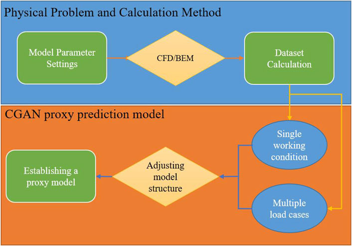
This paper primarily focuses on combining CGAN with traditional numerical simulation methods to predict the vibration noise of airfoil structures [42], reducing the cumbersome calculations involved in numerical methods and speeding up the prediction process of airfoil structure noise [43]. Figure 1 illustrates the process of establishing a surrogate model using CGAN.

Figure 1

Figure 1. Process of establishing a proxy prediction model for predicting wing structure noise.

2 Conditional generation adversarial neural network theory

2.1 Generate adversarial neural networks

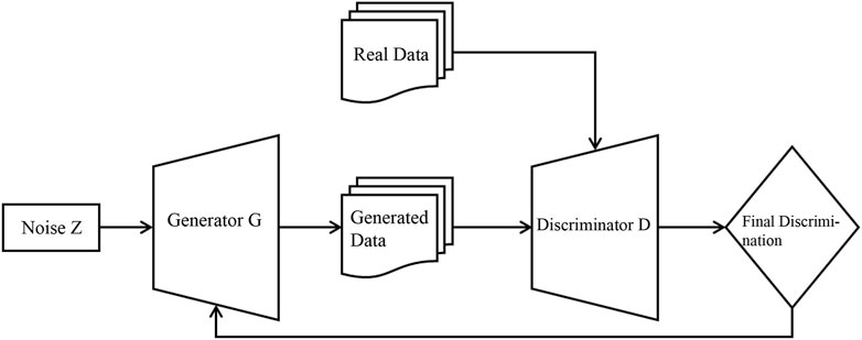
Generative Adversarial Networks (GAN) are an innovative technology that combines deep learning with probability theory. It consists of two competing neural networks that have the ability to learn independently and aims to learn and mimic the distribution of real data through unsupervised learning [44, 45]. The basic structure of GAN includes a generator and a discriminator, which compete against each other during the iterative training process. The objective is to make the generated data resemble the characteristics of real data as much as possible [46]. The generator is responsible for creating data that can deceive the discriminator by making it appear close to authentic data, the discriminator aims to distinguish between genuine and synthesized data. In this process, both sides continuously learn and self-optimize, aiming to reach the Nash equilibrium point in game theory, where the generated data is indistinguishable from real data. The flowchart of the GAN process is shown in Figure 2.

Figure 2

Figure 2. GAN process structure diagram.

The input to the generator model G is random noise z, and its output is a sample that resembles the distribution of real data. On the other hand, the input to the discriminator model D is either real data x or samples generated by G, denoted as G(z) [47]. When the input is x, the discriminator D outputs 1, and when the input is G(z), the discriminator D outputs 0. The abilities of G and D improve during the iterative training process and eventually reach an equilibrium state where D cannot distinguish between the two types of input data, indicating that the generator G has successfully approximated the distribution of real data [48]. The loss of GAN is closely related to the losses of G and D. The loss function of GAN is represented by Equation 1.

$\underset{G}{\min }\underset{D}{\max }V\left(D,G\right)=E_{x{P}_{\mathit{data}}\left(x\right)}\left[\log D\left(x\right)\right]+E_{z{P}_z\left(z\right)}\left[\log \left(1-D\left(G\left(z\right)\right)\right)\right](1)$

Both $P_{\mathit{data}}(\cdot )$ and $P_z(\cdot )$ represent the distribution of real data and noise data, respectively. In the training of GAN, the generator G is first fixed, and the discriminator D is trained with the main objective of improving D’s ability to discriminate between the two sources of data [49]. Then, the discriminator model is fixed, and the generator model is trained to generate data that can deceive the discriminator as much as possible. The introduction of GAN has provided more possibilities for the development of deep learning, receiving extensive attention from scholars worldwide at that time. However, GAN also has its limitations, such as asynchronous training of the generator and discriminator, low accuracy of generated data, high variability in generated data, and difficulty in reaching an equilibrium state. These issues restrict the application of GAN in various fields, especially in practical engineering scenarios where many problems cannot be directly solved by formulas. To address these issues, researchers have proposed derivative models such as CGAN, which incorporates conditional information into the GAN framework, transforming the originally unsupervised learning GAN into a supervised learning approach. This provides a direction for data generation in GAN and greatly expands its application areas. Many subsequent variants of GAN have been inspired by CGAN. Therefore, in this study, we have decided to use CGAN for noise data prediction. The following sections will provide a detailed introduction to CGAN.

2.2 Conditional generation adversarial neural network

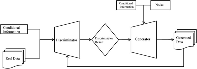
Conditional Generative Adversarial Networks (CGANs), developed by Mirza [13] introduce conditional variables into the model, which constrain the process of data generation and enable targeted generation of desired data. This model introduces conditional variables into the network architecture to guide the data generation process and achieve targeted generation of specific data. The CGAN architecture is similar to the original GAN [49], but with the addition of extra conditional variables, denoted as y, in both the generator G and discriminator D. This modification allows CGAN to operate as a controlled and supervised network model. The objective function of CGAN is presented in Equation 2, which incorporates conditional probabilities to form a constrained maximin function.

$\underset{G}{\min }\underset{D}{\max }V\left(D,G\right)=E_{x\sim P_{\text{data}}\left(x\right)}\left[\log D\left(x|y\right)\right]+E_{z\sim P_z\left(z\right)}\left[\log \left(1-D\left(G\left(z|y\right)\right)\right)\right](2)$

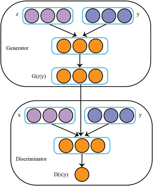
Figure 3 presents the CGAN model, which is built upon the core concept of Nash equilibrium derived from game theory. It mainly consists of two network structures, $G$ and $D$, which can be regarded as players in the game. $G$’s function is to learn data distribution features from real data as much as possible, and then generate false data that may confuse the discriminator. The primary role of the discriminator is to effectively differentiate between real and generated data, thereby accurately determining the source of the data. To outperform each other, both the generator and discriminator must continuously enhance and optimize their abilities. This iterative process of improvement and optimization in CGAN aims to achieve a Nash equilibrium between the two components. For the generation model $G$, its input is random noise $z$ and corresponding conditional information $y$, and its output is generated sample similar to real data distribution. The discriminator model $D$ is designed to take real data $x$, corresponding conditional information $y$, and generated sample $G(y,z)$ as inputs. It assigns an output of 1 or 0, depending on whether the input is real data or a generated sample, respectively. Its main function is a dichotomous test. The mutual game optimization process of generator $G$ and discriminator $D$ makes the ability of $D$ and $G$ continuously improve and finally reach an equilibrium state, that is, discriminator $D$ can no longer distinguish between the two types of input data. The training of CGAN is a process of $D$ and $G$ alternating repeatedly, so its loss function is closely related to the loss function of $D$ and $G$, which can be expressed as Equation 3:

$L\left(G,D\right)=E_{x,y,P_{\mathit{data}}\left(x,y\right)}\left[\log D\left(x,y\right)\right]+E_{y,p_y\left(y\right),z,p_z\left(z\right)}\left[\log \left(1-D\left(G\left(y,z\right),y\right)\right)\right](3)$

Figure 3

Figure 3. CGAN training flowchart.

where $P_{\mathit{data}}(x,y)$ represents the distribution of input data, $D$(.) and $G$(.) represent the output of $D$ and $G$ respectively, z is random noise. The loss function for $D$ and $G$ is written as Equation 5:

$L_D=-E_{x,y,p_{\mathit{data}}\left(x,y\right)}\left[\log D\left(x,y\right)\right]-E_{z,p_z,y,p_y\left(z,y\right)}\left[\log \left(1-D\left(G\left(z,y\right),y\right)\right)\right](4)$

$L_G=E_{z,p_z,y,p_y\left(z,y\right)}\left[\log \left(1-D\left(G\left(z,y\right)\right),y\right)\right](5)$

where $\tilde{u}\gg \mathrm{u}$, and when the prediction accuracy of the neural network is high enough. The optimal result of the predicted value can be considered as the optimization result of the original problem.

After the introduction of conditional variables y, the discriminator and generator in CGAN are responsible for distinguishing between real and generated data under the given condition and generating corresponding data, respectively. Figure 4 illustrates the training process of CGAN, where both the generator G and discriminator D take into account the additional information y as inputs.

Figure 4

Figure 4. Schematic diagram of CGAN structure: Generator $G$ and Discriminator $D$.

3 Acoustic boundary element method

First, the common Burton-Miller-based equation of boundary integral is employed to accurately evaluate the sound pressure field at broadband frequencies, as follows

$\begin{array}{cc}\hfill & C\left(\mathbf{x}\right)\left(p\left(\mathbf{x}\right)+\alpha q\left(\mathbf{x}\right)\right)+{\int }_{S}F\left(\mathbf{x},\mathbf{y}\right)p\left(\mathbf{y}\right)\mathrm{d}S\left(\mathbf{y}\right)+\alpha {\int }_{S}H\left(\mathbf{x},\mathbf{y}\right)p\left(\mathbf{y}\right)\mathrm{d}S\left(\mathbf{y}\right)\hfill \\ \hfill & ={\int }_{S}G\left(\mathbf{x},\mathbf{y}\right)q\left(\mathbf{y}\right)\mathrm{d}S\left(\mathbf{y}\right)+\alpha {\int }_{S}K\left(\mathbf{x},\mathbf{y}\right)q\left(\mathbf{y}\right)\mathrm{d}S\left(\mathbf{y}\right)+\left[p_{\text{inc}}\left(\mathbf{x}\right)+\alpha \frac{\partial p_{\mathrm{i}\mathrm{n}\mathrm{c}}\left(\mathbf{x}\right)}{\partial n\left(\mathbf{x}\right)}\right]\hfill \end{array}$

where $\alpha$ represents the coupling parameter: defined as $\alpha =\text{i}/k$ where $k>1$ and $\alpha =\text{i}$ in other cases. The symbol $k$ represents the wave number, where $k=c/\omega$, with $\omega$ being the angular frequency and $c$ being the speed of sound. When the point of source $\mathbf{x}$ is located on a border that is smooth $S$, $C(\mathbf{x})=1/2$, the sound pressure is indicated by $p(\mathbf{x})$, $p(\mathbf{y})$ represents the sound pressure at the field point $\mathbf{y}$, while $q(\mathbf{y})$ represents its normal derivative. $p_{\mathrm{i}\mathrm{n}\mathrm{c}}\left(\mathbf{x}\right)$ represents the plane wave’s incident acoustic pressure. The function of Green $G(\mathbf{x},\mathbf{y})$ and the equation given in Equation 6 and its corresponding derivative are defined as follows.

$\begin{array}{c}\hfill \left\{\begin{array}{c}G\left(\mathbf{x},\mathbf{y}\right)=\frac{\text{i}}{4}{H}_0^{\left(1\right)}\left(kr\right)\hfill \\ \hfill \\ F\left(\mathbf{x},\mathbf{y}\right)=\frac{\partial G\left(\mathbf{x},\mathbf{y}\right)}{\partial n\left(\mathbf{y}\right)}=-\frac{\text{i}k}{4}{H}_1^{\left(1\right)}\left(kr\right)\frac{\partial r}{\partial n\left(\mathbf{y}\right)}\hfill \\ \hfill \\ K\left(\mathbf{x},\mathbf{y}\right)=\frac{\partial G\left(\mathbf{x},\mathbf{y}\right)}{\partial n\left(\mathbf{x}\right)}=-\frac{\text{i}k}{4}{H}_1^{\left(1\right)}\left(kr\right)\frac{\partial r}{\partial n\left(\mathbf{x}\right)}\hfill \\ \hfill \\ H\left(\mathbf{x},\mathbf{y}\right)=\frac{{\partial }^{2}G\left(\mathbf{x},\mathbf{y}\right)}{\partial n\left(\mathbf{x}\right)\partial n\left(\mathbf{y}\right)}=\frac{\text{i}k}{4r}{H}_1^{\left(1\right)}\left(kr\right)n_j\left(\mathbf{x}\right)n_j\left(\mathbf{y}\right)\hfill \\ -\frac{\text{i}{k}^2}{4}{H}_2^{\left(1\right)}\left(kr\right)\frac{\partial r}{\partial n\left(\mathbf{x}\right)}\frac{\partial r}{\partial n\left(\mathbf{y}\right)}\hfill \end{array}\right.\end{array}(6)$

where $H_n^{(1)}(kr)$ represents the nth order Hankel function of the first kind for the Green’s function $G(x,y)$, $\mathrm{i}=\sqrt{-1}$, $r=|\mathbf{x}-\mathbf{y}|$ represents the distance between the source and field points, $n_j$ is the Cartesian component of $n(\mathbf{x})$ or $n(\mathbf{y})$ and $\partial r/\partial n=r_{,j}{n}_j$.

The boundary of the structure’s surface is discretized using constant elements. Subsequently, after gathering all the collocation points (nodes) at the center of each element, Equation 6 is reformulated in matrix form as follows.

$\mathbf{H}\mathbf{p}=\mathbf{G}\mathbf{q}+{\mathbf{p}}_{\text{inc}}(7)$

In the above equation, H and G represent the coefficient matrices utilized in the BEM. These matrices are characterized by their high density and non-symmetry, and they also exhibit frequency-dependent variations. The vectors $p$ and $q$ are denoted by $\mathbf{p}$ and $\mathbf{q}$ respectively, and ${\mathbf{p}}_{\text{inc}}$ represents the incident wave vector. Taking into account the impedance boundary condition $q(\mathbf{x})=\text{i}k\beta (\mathbf{x})p(\mathbf{x})$, Equation 7 can be rewritten as

$\mathbf{p}={\mathbf{p}}_{\mathrm{i}\mathrm{n}\mathrm{c}}(8)$

in which the diagonal matrix $\mathbf{B}$ can be expressed as Equation 9.

$\mathbf{B}=\text{i}k\left[\begin{array}{ccc}\hfill {\beta }_1\hfill & \hfill \cdots \hfill & \hfill 0\hfill \\ \hfill ⋮\hfill & \hfill \ddots \hfill & \hfill ⋮\hfill \\ \hfill 0\hfill & \hfill \cdots \hfill & \hfill {\beta }_n\hfill \end{array}\right](9)$

where the normalized acoustic impedance value of the ith element is represented by ${\beta }_i$. Incorporating the external sound field, the sound pressure ${\mathbf{p}}_f$ can be represented as Equation 10.

${\mathbf{p}}_f=-\left[{\mathbf{H}}_f-{\mathbf{G}}_f\mathbf{B}\right]\mathbf{p}+{\mathbf{p}}_f^{\mathrm{i}\mathrm{n}\mathrm{c}}(10)$

where akin to the coefficient matrix in Equation 7, ${\mathbf{H}}_f$ and ${\mathbf{G}}_f$ stand for the coefficient matrices corresponding to field points $\mathbf{y}$ situated in the external acoustic domain. The Taylor expansion of the $n$-th order Hankel function of the first kind at the frequency $z_0=k_{0}r$ is given by

$H_n^{\left(1\right)}\left(z\right)={\displaystyle \sum _{m=0}^{\infty }}\frac{{\left(z-z_{0}r\right)}^m}{m!}{\left[H_n^{\left(1\right)}\left(z\right)\right]}_{z=z_0}^{\left(m\right)}(11)$

in which ${\left[H_n^{(1)}(z)\right]}_{z=z_0}^m={\left.\frac{{\mathrm{d}}^m{H}_n^{(1)}(z)}{\mathrm{d}{z}^m}\right|}_{z=z_0}$. Replacing $z$ and $z_0$ with $kr$ and $k_{0}r$ respectively, we obtain the Taylor series expansion of the kernel function in Equation 6. As deriving an explicit expression for the $m$-th derivative of the $n$-th order Hankel function is highly intricate, this paper uses the recursive form as in Equation 12.

$\frac{\mathrm{d}{H}_n^{\left(1\right)}\left(z\right)}{\mathrm{d}z}=\frac{n}{z}{H}_n^{\left(1\right)}\left(z\right)-H_{n+1}^{\left(1\right)}\left(z\right)(12)$

Through successive differentiations with respect to the variable $z$, we derive the recursive expression for the $m$-th derivative of the $n$-th order Hankel function.

${\left[H_n^{\left(1\right)}\left(z\right)\right]}^{\left(m\right)}={\displaystyle \sum _{i=1}^m}{\left[H_n^{\left(1\right)}\left(z\right)\right]}^{\left(m-i\right)}\frac{{\left(-1\right)}^{i+1}\left(m-1\right)!}{z^i\left(m-i\right)!}-{\left[H_{n+1}^{\left(1\right)}\left(z\right)\right]}^{\left(m-1\right)}(13)$

Next, by substituting Equation 13 into Equation 11, we derive the expansion of $H_n^{(1)}(kr)$ at point $k_0$.

Combining Equations 6, 11, we can derive the expansion of the integral in Equation 4 at the point $\mathbf{y}$ as follows

$\begin{array}{c}\hfill \begin{array}{cc}\hfill & {\int }_{S}F\left(\mathbf{x},\mathbf{y}\right)p\left(\mathbf{y}\right)\mathrm{d}S\left(\mathbf{y}\right)={\displaystyle \sum _{m=0}^{\infty }}\frac{{\left(k-k_0\right)}^m}{m!}{I}_1^m\hfill \\ \hfill & {\int }_{S}G\left(\mathbf{x},\mathbf{y}\right)q\left(\mathbf{y}\right)\mathrm{d}S\left(\mathbf{y}\right)={\displaystyle \sum _{m=0}^{\infty }}\frac{{\left(k-k_0\right)}^m}{m!}k{I}_2^m\hfill \\ \hfill & \alpha {\int }_{S}H\left(\mathbf{x},\mathbf{y}\right)p\left(\mathbf{y}\right)\mathrm{d}S\left(\mathbf{y}\right)={\displaystyle \sum _{m=0}^{\infty }}\frac{{\left(k-k_0\right)}^m}{m!}\left(k{I}_3^m+k^2{I}_4^m\right)\hfill \\ \hfill & \alpha {\int }_{S}K\left(\mathbf{x},\mathbf{y}\right)q\left(\mathbf{y}\right)\mathrm{d}S\left(\mathbf{y}\right)={\displaystyle \sum _{m=0}^{\infty }}\frac{{\left(k-k_0\right)}^m}{m!}{k}^2{I}_5^m\hfill \end{array}\end{array}(14)$

where

$\begin{array}{cc}\hfill & I_1^m=-{\int }_S\frac{\text{i}{r}^{m-1}}{4}{\left[z{H}_1^{\left(1\right)}\left(z\right)\right]}_{z=k_{0}r}^{\left(m\right)}\frac{\partial r}{\partial n\left(\mathbf{y}\right)}p\left(\mathbf{y}\right)\mathrm{d}S\left(\mathbf{y}\right)\hfill \\ \hfill & I_2^m=-{\int }_S\frac{{\beta }_i{r}^m}{4}{\left[H_0^{\left(1\right)}\left(z\right)\right]}_{z=k_{0}r}^{\left(m\right)}p\left(\mathbf{y}\right)\mathrm{d}S\left(\mathbf{y}\right)\hfill \\ \hfill & I_3^m={\int }_S\frac{\alpha \text{i}{r}^{m-1}}{4}{\left[H_1^{\left(1\right)}\left(z\right)\right]}_{z=k_{0}r}^{\left(m\right)}{n}_j\left(\mathbf{x}\right)n_j\left(\mathbf{y}\right)p\left(\mathbf{y}\right)\mathrm{d}S\left(\mathbf{y}\right)\hfill \\ \hfill & I_4^m={\int }_S\frac{\alpha \text{i}{r}^m}{4}{\left[H_2^{\left(1\right)}\left(z\right)\right]}_{z=k_{0}r}^{\left(m\right)}\frac{\partial r}{\partial n\left(\mathbf{x}\right)}\frac{\partial r}{\partial n\left(\mathbf{y}\right)}p\left(\mathbf{y}\right)\mathrm{d}S\left(\mathbf{y}\right)\hfill \\ \hfill & I_5^m={\int }_S\frac{\alpha {\beta }_i{r}^m}{4}{\left[H_1^{\left(1\right)}\left(z\right)\right]}_{z=k_{0}r}^{\left(m\right)}\frac{\partial r}{\partial n\left(\mathbf{y}\right)}p\left(\mathbf{y}\right)\mathrm{d}S\left(\mathbf{y}\right)\hfill \end{array}(15)$

In the integral $I_1^m$, the $m$-th derivative of the function $z{H}_1^{(1)}(z)$ is represented as Equation 16.

${\left[\left(z\right)H_1^{\left(1\right)}\left(z\right)\right]}^{\left(m\right)}=m{\left[H_1^{\left(1\right)}\left(z\right)\right]}^{\left(m-1\right)}+z{\left[H_1^{\left(1\right)}\left(z\right)\right]}^{\left(m\right)}(16)$

Substituting Equations 14, 15 into Equation 6 with impedance boundary conditions, we derive the following expression.

$C\left(\mathbf{x}\right)p\left(\mathbf{x}\right)\left(1+\alpha \text{i}k\beta \left(\mathbf{x}\right)\right)+{\displaystyle \sum _{m=0}^{\infty }}\frac{{\left(k-k_0\right)}^m}{m!}\left[I_1^m+k\left(-I_2^m+I_3^m\right)+k^2\left(I_4^m-I_5^m\right)\right]=\left[p_{\text{inc}}\left(x\right)+\alpha \frac{\partial p_{\text{inc}}\left(x\right)}{\partial n\left(\mathbf{x}\right)}\right](17)$

Due to the presence of singularity in the kernel function and its normal derivative in Equation 6, not only is the behavior of this equation affected but it also has an impact on other associated expressions. Consequently, the boundary integrals involving a series of expansions in Equation 15 also exhibit singularity. Standard integration methods are insufficient to solve these singular integrals. Instead, techniques such as Cauchy principal value and Hadamard finite part integral must be employed to handle them.

To discretize Equation 17, the collocation method can be utilized along with constant elements. This results in the following expression.

$\mathbf{C}\mathbf{p}+k\bar{\mathbf{C}}p+{\displaystyle \sum _{m=0}^{\infty }}\frac{{\left(k-k_0\right)}^m}{m!}\left[{\mathbf{I}}_1^m+k{\mathbf{I}}_2^m+k^2{\mathbf{I}}_3^m\right]\mathbf{p}={\mathbf{P}}_{\mathit{inc}}(18)$

where C matrix can be expressed in the form of Equation 19.

$\begin{array}{c}\hfill \mathbf{C}=\left[\begin{array}{ccc}\hfill C_1\hfill & \hfill \hfill & \hfill \mathbf{0}\hfill \\ \hfill \hfill & \hfill \ddots \hfill \\ \hfill \mathbf{0}\hfill & \hfill \hfill & \hfill C_N\hfill \end{array}\right]\mathrm{a}\mathrm{n}\mathrm{d}\bar{\mathbf{C}}=\alpha \mathrm{i}\left[\begin{array}{ccc}\hfill {\beta }_1{C}_1\hfill & \hfill \hfill & \hfill \mathbf{0}\hfill \\ \hfill \hfill & \hfill \ddots \hfill \\ \hfill \mathbf{0}\hfill & \hfill \hfill & \hfill {\beta }_N{C}_N\hfill \end{array}\right]\end{array}(19)$

Let matrices ${\tilde{\mathbf{I}}}_1^m$ and ${\tilde{\mathbf{I}}}_2^m$ be defined as Equation 20.

$\begin{array}{c}\hfill {\tilde{\mathbf{I}}}_1^m=\left\{\begin{array}{cc}\mathbf{C}+{\mathbf{I}}_1^0,\hfill & m=0\hfill \\ {\mathbf{I}}_1^m,\hfill & m\ne 0\hfill \end{array}\right.\mathrm{a}\mathrm{n}\mathrm{d}{\tilde{\mathbf{I}}}_2^m=\left\{\begin{array}{cc}\bar{\mathbf{C}}+{\mathbf{I}}_2^0,\hfill & m=0\hfill \\ {\mathbf{I}}_2^m,\hfill & m\ne 0\hfill \end{array}\right.\end{array}(20)$

Then, by setting ${\mathbf{I}}_3^m={\tilde{\mathbf{I}}}_3^m$, Equation 18 can be redefined as Equation 21.

$\left[{\displaystyle \sum _{m=0}^M}\frac{{\left(k-k_0\right)}^m}{m!}\left({\tilde{\mathbf{I}}}_1^m+k{\tilde{\mathbf{I}}}_2^m+k^2{\tilde{\mathbf{I}}}_3^m\right)\right]\mathbf{p}={\tilde{\mathbf{P}}}_{\mathit{inc}}(21)$

This expression includes only the initial $M$ terms of the Taylor expansion. Since matrices ${\tilde{\mathbf{I}}}_1^m$, ${\tilde{\mathbf{I}}}_2^m$, and $\widetilde{{\mathbf{I}}_3^m}$ are not influenced by frequency, they can be computed just once for wideband acoustic analysis. This helps to eliminate the significant computational cost associated with repeatedly calculating Equation 8 for different frequencies.

4 Numerical examples

In this section, the validation of the previously proposed methods was conducted [50]. First, the BEM method was verified, followed by the establishment of the BEM-CGAN wing noise surrogate prediction model based on BEM data integrated with CGAN. Additionally [51–53], the CAA-CGAN model validation was performed, along with the prediction of a propeller wake model.

4.1 The wing structural vibration and noise prediction model based on BEM-CGAN

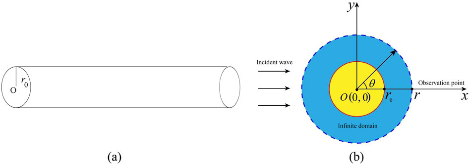
First, consider the two-dimensional acoustic field calculation model of the tubular structure as shown in Figure 5. Let $r_0$ be the radius of the cylindrical shell. In the acoustic field calculation, a normal velocity $v_0$ = 9.6$\times 10^{-5}$m/s is provided, which is generated by the internal pressure of the pipe wall. The boundary condition is set at the observation point r (2 m, 0 m).

Figure 5

Figure 5. (A) Tubular structure; (B) Section diagram.

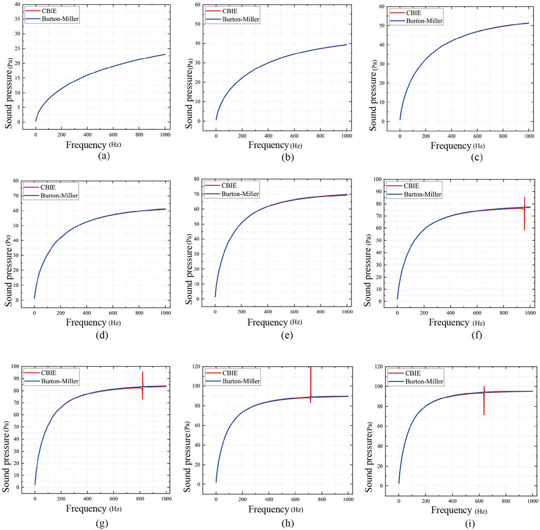
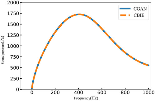
The 2D cylindrical shell surface is uniformly discretized into 100 constant elements. When the pipe radius r0 is set to 100, 150, 200 … , 900 mm, and the frequency f ranges from 0 to 1000 Hz (with a step size of 1 Hz), Figure 6 presents the frequency response curves of sound pressure amplitudes computed using the conventional boundary element method (referred to as CBIE) and the Burton-Miller method. From Figure 6, several conclusions can be drawn: as the pipe radius increases, the sound pressure at the observation location also increases. The results obtained using the CBIE method and the Burton-Miller method are essentially the same. However, when the radius $r_0\ge 600\mathrm{m}\mathrm{m}$, the CBIE method exhibits false peak issues, while the Burton-Miller method can effectively resolve this problem.

Figure 6

Figure 6. $r_0$ = 100,200, CBIE and Burton-Miller method for sound pressure calculation at 900 mm (A–I).

The comparison between the Taylor expansion method and the analytical solution is shown in Figure 7. The acoustic pressure results for different pipe structure radii $r_0$ were obtained using the Taylor expansion-based boundary element method in the frequency range of [1, 1,000] Hz with a frequency step size of 1 Hz.

Figure 7

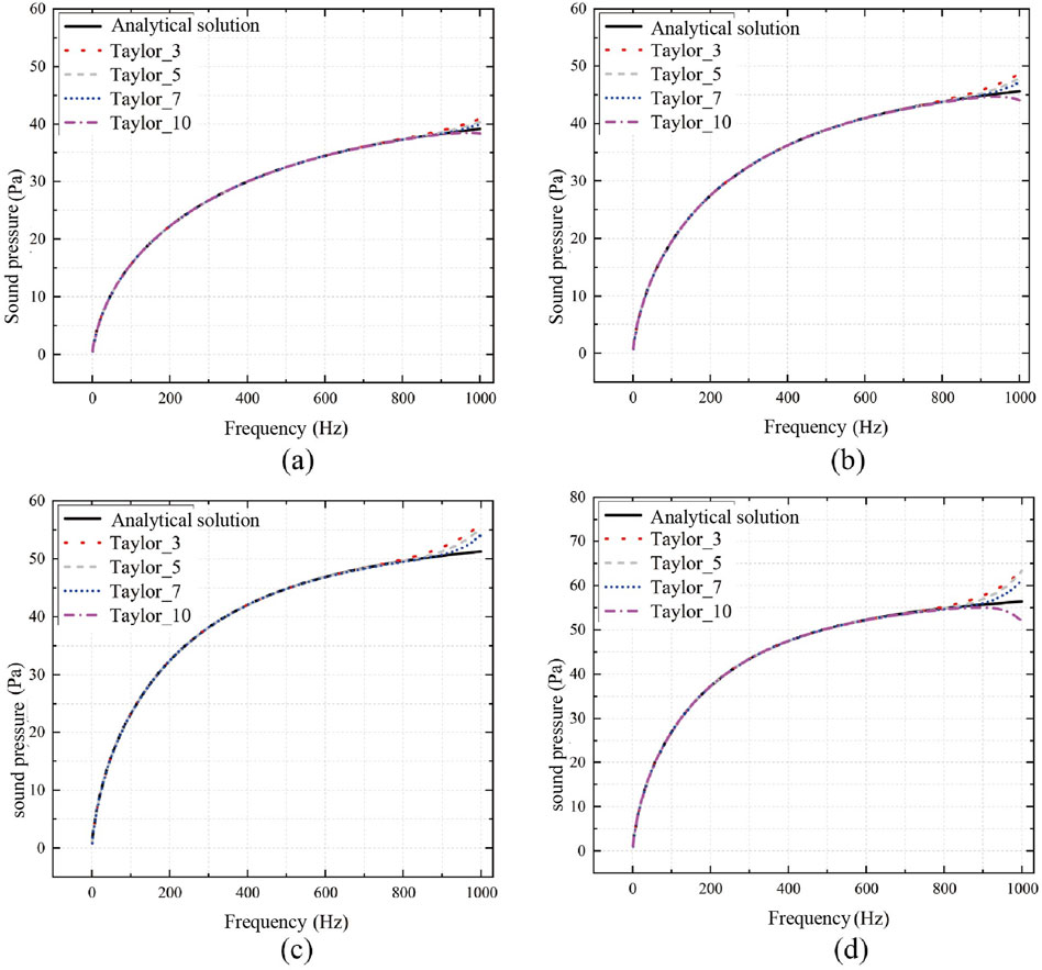
Figure 7. Sound pressure calculation results of Taylor’s expansion method and analytical solutions for tubular structures. (A): r₀ = 200 mm; (B) r₀ = 250 mm; (C) r₀ = 300 mm; (D) r₀ = 350 mm.

From Figure 7, it is evident that as the number of terms in the Taylor expansion increases, the numerical solution approaches the analytical solution more closely. Notably, there are substantial disparities in the boundaries of the frequency range, primarily because the fixed frequency expansion point is positioned in the middle of the frequency range. The numerical results become increasingly inaccurate as one moves farther away from the fixed frequency expansion point. To validate this hypothesis, simulations were conducted for the radius $r_0$ = 400 mm with frequency ranges of [1, 250] Hz and [250, 500] Hz. Figure 8 presents the simulated results.

Figure 8

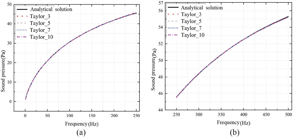
Figure 8. Sound pressure calculation results of Taylor’s expansion method and analytical solution at [1,500]Hz when $r_0$ = 400 mm. (A) Frequency at [0,250]; (B) Frequency at [250,500].

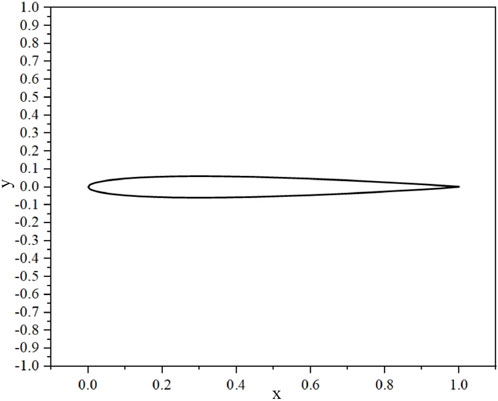
So far, the numerical methods used in this study have been validated. Next, these methods will be applied to simulate the airfoil structure, providing sample data for the construction of the BEM-CGAN model. The airfoil model used in this study is the NACA0012 airfoil, and its structure is shown in Figure 9.

Figure 9

Figure 9. NACA0012 airfoil structure diagram.

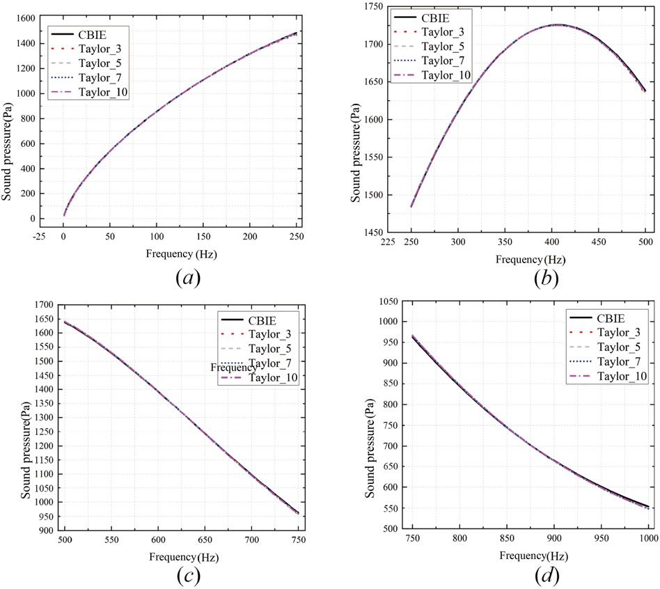
The sound pressure in the frequency range of [1–1,000] Hz, the first approach utilized is the CBIE method together with the fast sweeping method, both of which rely on Taylor expansion. This frequency band is further divided into [1–250], [250–500], [500–750], and [750–1,000]. Then, these two methods are used for simulation, and the results are shown in Figure 10.

Figure 10

Figure 10. Frequency segmentation simulation results [(A–D): 1–1000 Hz].

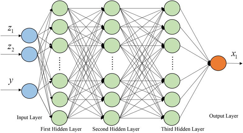
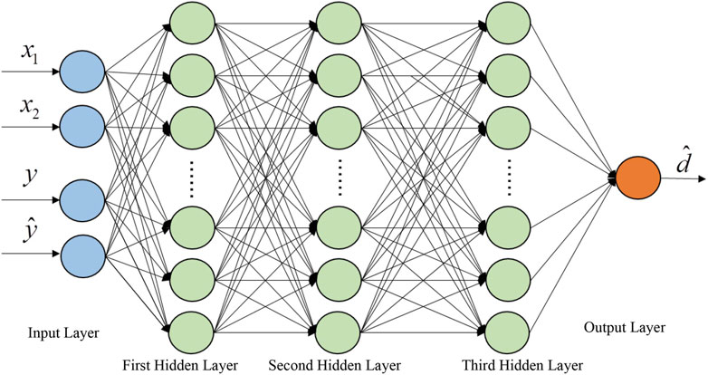
Based on Figure 10, it can be observed that as the frequency band decreases, the error between the results obtained from the fast sweeping method based on Taylor expansion and the CBIE method decreases. Therefore, we can conclude that as the frequency band becomes smaller, the results obtained from the fast sweeping method based on Taylor expansion become closer to the true solution. At this point, the obtained samples can serve as the foundation for training the CGAN model. Next, let’s analyze the modeling and prediction results of the CGAN model using the airfoil structure in the [1–1,000] Hz frequency range as an example. For the noise prediction problem of the airfoil, the discriminator and generator of the CGAN can be viewed as regression models. Therefore, the Mean Squared Error (MSE) function is selected as the loss function, and the Sigmoid function is chosen as the activation function. The capability of the generator and discriminator should approach a balance, and the representation has a relatively small parameter dimension. Thus, both the generator and discriminator adopt fully connected neural networks with three hidden layers. The network structure configuration for the CGAN model is presented in Table 1, and the schematic diagram of the network structure is shown in Figures 11, 12. The general modeling flowchart of machine learning is shown in Figure 13.

Table 1

Table 1. Network structure and training parameter setting of CGAN.

Figure 11

Figure 11. Network architecture of CGAN’s generator.

Figure 12

Figure 12. Network architecture of CGAN’s discriminator.

Figure 13

Figure 13. General modeling flowchart of machine learning.

In Figure 11, $z_1$ and $z_2$ represent the random vectors input to the generator. $y$ represents the label information, where in this case it corresponds to the frequency information. $x_1$ represents the generated data, which is the sound pressure at the observation points. In the discriminator, $x_2$ represents the real data, apologies for the confusion. In the discriminator, $\widehat{y}$ represents the label information, specifically the frequency information. $\widehat{d}$ represents the judgment result of the discriminator’s output layer, indicating the discriminator’s classification of the input as real or fake. $x_2$ represents the real data. The machine learning modeling in this study was conducted on a desktop workstation with the following specifications: Windows Server 2019 as the operating system, 32 GB of memory, an NVIDIA GeForce RTX 4090 GPU, TensorFlow-GPU 2.6.0 as the development framework, and Python as the programming language. The detailed contents can be found in Table 2. After setting the CGAN parameters, the sound pressure data of the wing structure calculated by CBIE in the frequency range of [1, 1,000] Hz was used as the dataset and input into CGAN for training. The testing dataset was also set to be the same as the training dataset to validate the applicability of CGAN. The predicted results are shown in Figure 14. From the figure, it can be seen that the predictions of CGAN align well with CBIE itself, indicating a good agreement. Subsequently, the next step of testing was performed by extracting 3/4 of the data from the CBIE dataset as the training set and the remaining 1/4 of the data as the testing set to evaluate the generalization performance of the CGAN model. Supplementary Figure 1 illustrates the performance of CGAN on the testing set. From the figure, it can be observed that the predicted results of CGAN on the testing set exhibit a good consistency with CBIE itself, demonstrating that CGAN can be applied in the field of regression prediction. These results validate the effectiveness and generalization capability of the CGAN model in predicting the sound pressure data of the wing structure.

Table 2

Table 2. Development environment parameters table.

Figure 14

Figure 14. Prediction results of CGAN on the CBIE dataset for airfoil structure.

4.2 Interference noise prediction model for wing vortex with CAA-CGAN

In the next step, the data obtained from simulating the structural vortex interference noise of the wing using computational aeroacoustics (CGAA) method is combined with CGAN to establish a proxy prediction model called CAA-CGAN [12]. The NACA0012 airfoil is chosen as the reference airfoil, having a thickness of 0.12c, degree of deflection 0.02c, and an angle of attack $a=2^{◦}$, where c represents the chord length of the airfoil. k is a wave number vector and $\epsilon$ is a small parameter, satisfy $\epsilon \ll 1$. The model and grid are shown in Figure 15.

Figure 15

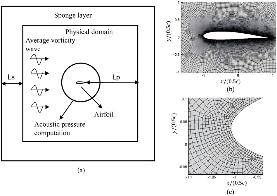
Figure 15. Examples of two-dimensional meshes used in current research. (A) Sketch the computational domain. (B) The grid near the wings. (C) Enlarged view near the leading edge.

For wind speed with wave numbers $k_1$ = $k_2$ = 1, Figure 16 presents the average wall pressure ${\mathrm{P}}_{\mathit{wall}}$ and root-mean-square and compares them with the benchmark reference values provided by [54].

Figure 16

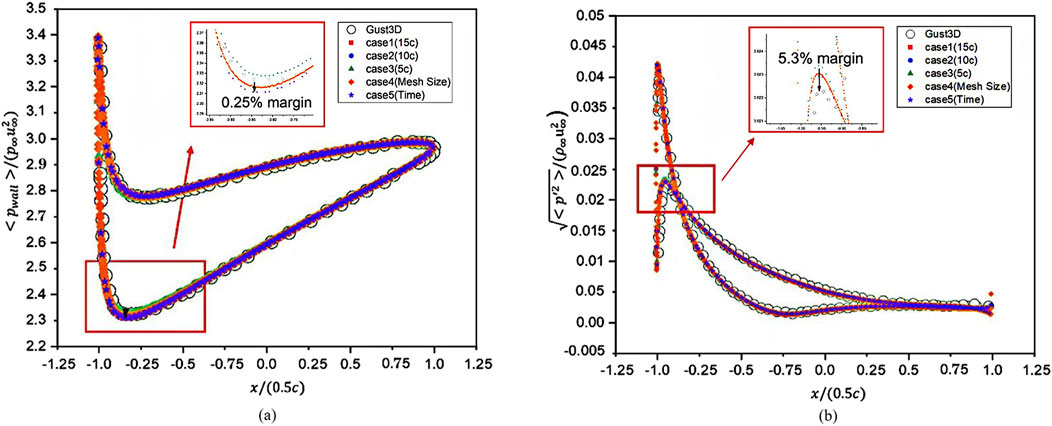
Figure 16. (A) average pressure distribution on the airfoil surface and (B) RMS pressure on the airfoil surface.

Based on the observation from the graph, we believe that the data obtained from CAA calculations is accurate and effective, making it suitable for training data in the subsequent CGAN modeling. Next, we will proceed with the establishment of the CAA-CGAN model. The configuration information is set as follows: for wave numbers k = 1,4,8, Ma = 0.1, 0.2, … , 0.7, and the far-field angles of the airfoil are considered as conditional information. The output data will be the calculated sound pressure from the CAA.

First, the generalization prediction ability of CGAN under a single operating condition is tested. The Mach number (Ma) and far-field azimuth are used as conditional information, and the far-field sound pressure data is considered as the data to be generated. For each operating condition, the dataset is divided into a 9:1 ratio for training and testing. The CGAN is used to learn and predict the CAA dataset, and the outcomes are then contrasted with the forecasts made by the Amiet theory. Figure 17 shows the far-field sound pressure results at different wave numbers for a Mach number of 0.5, on a circular region with a radius of 4c.

Figure 17

Figure 17. Comparison of far-field sound pressure prediction results when wave number k = 1,4,8 and Mach number Ma = 0.5.

After conducting the generalization testing, we extend the predictive model to predict the far-field sound pressure data under unknown operating conditions. The specific procedure is as follows: we extract the data from the training set at wave numbers k = 1, 4, 8, and Mach number Ma = 0.5, and use it as the test set. We evaluate the accuracy of the CAA-CGAN predictive model when predicting far-field sound pressure data under unknown operating conditions. Figure 18 presents a comparison of the predictive results from CGAN, CAA, and the predictions based on Amiet theory.

Figure 18

Figure 18. Comparison of prediction results of CGAN on sound pressure data under unknown working conditions.

From the graph, it can be observed that the predictive results from CGAN align well with the data from CAA, and the accuracy is stronger compared to the results obtained from Amiet theory.

4.3 Regarding the prediction of the velocity profile of a propeller wake

Finally, we validate the model using an example of a propeller wake. The model structure, as shown in Figure 19A, divided the domain into 12 million grids. RANS algorithm was employed in the simulation using Numeca software. The detailed diagram of the model is presented in Figure 19B. Firstly, we verified the effectiveness of CGAN in predicting the flow field data of a propeller under a single operating condition. Then, we considered using CGAN to predict the velocity distribution and key parameters of the propeller wake under multiple operating conditions. In this example, the main operating condition information considered was the wind speed and propeller rotation speed.

Figure 19

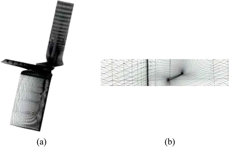
Figure 19. Schematic Diagram of the Contra-Rotating Propeller Grid Model and Local View of the Rear Blade: (A) Regarding the mesh model of a propeller; (B) Regarding the local image of a propeller’s trailing blade.

Firstly, under fixed wind speed and rotation speed conditions, the three-dimensional flow field of the propeller wake was divided into 13 planes. The velocity distribution at the trailing edge of the rear propeller blade was extracted. CGAN was used for the adaptability test of predicting the velocity distribution and semi-wake width of the propeller wake. The input and output parameters of CGAN are shown in Table 3.

Table 3

Table 3. Input and output variables of CGAN under single operating conditions.

Secondly, we verify the applicability of CGAN by testing it on the training dataset itself. The data from the cases with a wind speed of 30 m/s and a rotation speed of 2,500 r/min are selected as the overall dataset. A portion of the wind speed distribution data from these cases is chosen as the training and testing sets. After 2,000 iterations of training, the predictive results of CGAN are shown in Figure 20.

Figure 20

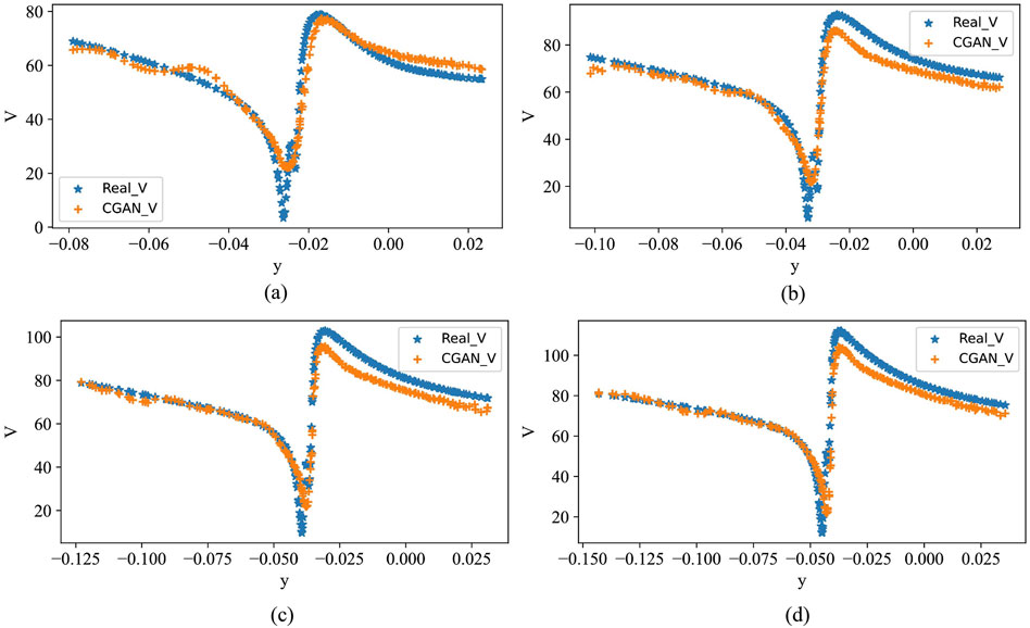
Figure 20. The velocity distribution on the tangent line of the leading edge of the rear blade of a counter rotating propeller (wind speed:30 m/s,rotational speed:2500 r/min). (A) Cross-Section 1; (B) Cross-Section 2; (C) Cross-Section 3; (D) Cross-Section 4.

Testing on the dataset under a single operating condition indicates that CGAN has the potential to be applied to such problems. Therefore, further exploration of CGAN’s generalization performance is needed.

From a practical perspective, what we often need is complete data for any operating condition, rather than partial data for specific conditions. Therefore, both the wind speed and velocity will be used as input variables, while other settings will be similar to before. Following the previous applicability test, the next step is to directly perform generalization testing. After multiple rounds of debugging, the number of hidden layers in CGAN has been increased to 10. The overall dataset consists of 27 sets of data under varying wind speeds and rotation speeds. The data with a wind speed of 50 m/s and a rotation speed of 5,500 r/min are selected as the testing set, and the results after 20,000 iterations of training are shown in Figure 21.

Figure 21

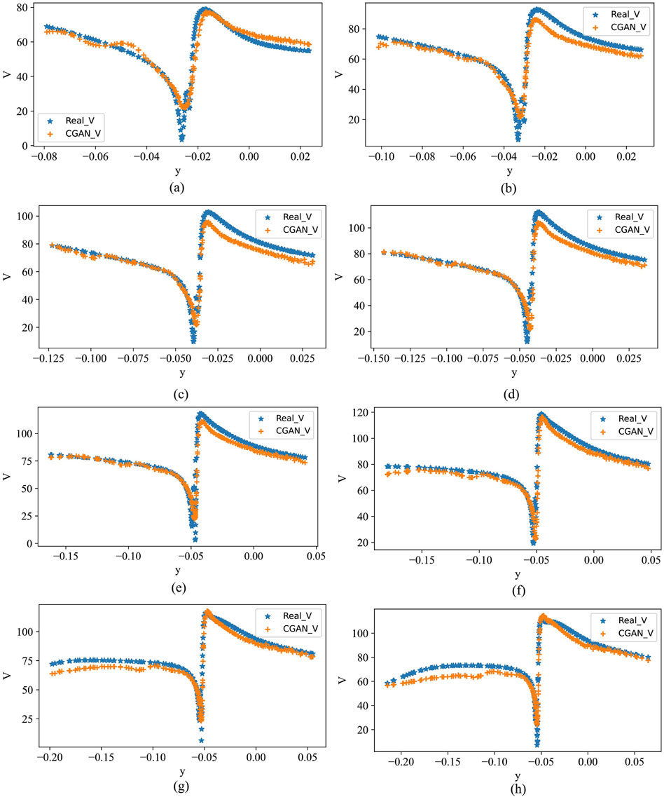
Figure 21. Prediction results of CGAN on a test set with wind speed of 50 $m/s$ and rotational speed of 5,500 $r/min$. (A) Cross-Section 1; (B) Cross-Section 2; (C) Cross-Section 3; (D) Cross-Section 4; (E) Cross-Section 5; (F) Cross-Section 6; (G) Cross-Section 7; (H) Cross-Section 8.

Figure 21 shows the velocity distribution along the tangential plane at 10 cross-sections of the propeller’s leading edge under the experimental conditions, yielding fairly accurate results. Additionally, we also predicted the velocity loss and half-wake width at a wind speed of 30 m/s and rotational speed of 4,800 rpm. The predicted results by the CGAN are shown in Figure 22.

Figure 22

Figure 22. Comparison between CGAN’s predicted results on the test set and the actual results: (A) The speed prediction results of CGAN; (B) Prediction results of half wake width for CGAN.

In Figure 22A shows the summary prediction results of the CGAN for velocity, while Figure 22B shows the summary results for the half-wake width. The half-wake width data was obtained through simple calculations on the initial data. The horizontal axis represents the test points corresponding to 13 cross-sections under this operating condition.

It is worth mentioning that when using CGAN to establish a surrogate prediction model, the generator of CGAN has an important parameter: the noise vector. In previous applications for image generation, this vector often had dozens or even hundreds of dimensions to ensure the richness of generated images. However, in the present study, a high-dimensional noise vector would not only lead to some generated data deviating from the desired results, but also significantly increase the complexity of the network structure in order to meet the accuracy requirements.

5 Conclusion

This study combines three numerical methods with Conditional Generative Adversarial Networks (CGANs) to establish a surrogate modeling approach for predicting the noise of airfoil structures. The main findings are as follows:

(1) The combination of BEM, CAA, CFD, and CGANs has been explored to investigate the applicability of CGANs to this type of problem.

(2) The surrogate prediction model established through CGANs reduces significant computation time, aiding in speeding up the optimization and design process of airfoil structures.

(3) Modifying certain structures of CGANs proves beneficial for handling regression problems in this research.

However, this approach has some limitations. It may struggle to achieve ideal prediction results when the data dimension is too high or when there is poor correlation between the data, rendering the predictions unreliable. To address these limitations, our future research will focus on developing more efficient numerical algorithms. Additionally, exploring advanced deep learning techniques to improve the accuracy of the surrogate model. By doing so, we aim to overcome these challenges and enhance the reliability and accuracy of the surrogate prediction model.

Data availability statement

The original contributions presented in the study are included in the article/Supplementary Material, further inquiries can be directed to the corresponding authors.

Author contributions

SJ: Writing–review and editing, Writing–original draft. YL: Writing–review and editing, Writing–original draft. YC: Writing–original draft. LG: Writing–original draft.

Funding

The author(s) declare that financial support was received for the research, authorship, and/or publication of this article. This research was supported by the State Key Laboratory of Aerodynamics (Grant No. SKLA2022KFKT007), and the Laboratory of Aerodynamic Noise Control (Grant No. ANCL 20230306).

Conflict of interest

The authors declare that the research was conducted in the absence of any commercial or financial relationships that could be construed as a potential conflict of interest.

Publisher’s note

All claims expressed in this article are solely those of the authors and do not necessarily represent those of their affiliated organizations, or those of the publisher, the editors and the reviewers. Any product that may be evaluated in this article, or claim that may be made by its manufacturer, is not guaranteed or endorsed by the publisher.

Supplementary material

The Supplementary Material for this article can be found online at: https://www.frontiersin.org/articles/10.3389/fphy.2024.1452876/full#supplementary-material

SUPPLEMENTARY FIGURE 1 | Comparison of CGAN’s prediction results on the test set with CBIE results.

References

1. Hubbard HH. Sound from dual-rotating and multiple single-rotating propellers. Tech Rep (1948).

Google Scholar

2. Parry AB. Theoretical prediction of counter-rotating propeller noise. University of Leeds (1988). Ph.D. thesis.

Google Scholar

3. Qu Y, Zhou Z, Chen L, Lian H, Li X, Hu Z, et al. Uncertainty quantification of vibro-acoustic coupling problems for robotic manta ray models based on deep learning. Ocean Eng (2024) 299:117388. doi:10.1016/j.oceaneng.2024.117388

CrossRef Full Text | Google Scholar

4. Marburg S, Schneider S. Performance of iterative solvers for acoustic problems. Part I. Solvers and effect of diagonal preconditioning. Eng Anal Boundary Elem (2003) 27:727–50. Special issue on Acoustics. doi:10.1016/S0955-7997(03)00025-0

CrossRef Full Text | Google Scholar

5. Marburg S, Hardtke H-J. Shape optimization of a vehicle hat-shelf: improving acoustic properties for different load cases by maximizing first eigenfrequency. Comput and Structures (2001) 79:1943–57. doi:10.1016/S0045-7949(01)00107-9

CrossRef Full Text | Google Scholar

6. Kostas K, Ginnis A, Politis C, Kaklis P. Ship-hull shape optimization with a T-spline based BEM—isogeometric solver. Computer Methods Appl Mech Eng (2015) 284:611–22. Isogeometric Analysis Special Issue. doi:10.1016/j.cma.2014.10.030

CrossRef Full Text | Google Scholar

7. Lian H, Wu P. The shape optimization of underground caverns based on strain energy criterion via explicit interface tracking methods. Int J Adv Eng Sci Appl Mathematics (2020) 12:183–92. doi:10.1007/s12572-020-00281-7

CrossRef Full Text | Google Scholar

8. Li S, Trevelyan J, Wu Z, Lian H, Wang D, Zhang W. An adaptive SVD-Krylov reduced order model for surrogate based structural shape optimization through isogeometric boundary element method. Computer Methods Appl Mech Eng (2019) 349:312–38. doi:10.1016/j.cma.2019.02.023

CrossRef Full Text | Google Scholar

9. Liu Z, Bian P, Qu Y, Huang W, Chen L, Chen J, et al. A galerkin approach for analysing coupling effects in the piezoelectric semiconducting beams. Eur J Mechanics-A/Solids (2024) 103:105145. doi:10.1016/j.euromechsol.2023.105145

CrossRef Full Text | Google Scholar

10. Lian H, Kerfriden P, Bordas S. Implementation of regularized isogeometric boundary element methods for gradient-based shape optimization in two-dimensional linear elasticity. Int J Numer Methods Eng (2016) 106:972–1017. doi:10.1002/nme.5149

CrossRef Full Text | Google Scholar

11. Jin Y, Hou L, Lu Z, Chen Y. Crack fault diagnosis and location method for a dual-disk hollow shaft rotor system based on the radial basis function network and pattern recognition neural network. Chin J Mech Eng (2023) 36:35. doi:10.1186/s10033-023-00856-y

CrossRef Full Text | Google Scholar

12. Cao G, Yu B, Chen L, Yao W. Isogeometric dual reciprocity bem for solving non-fourier transient heat transfer problems in fgms with uncertainty analysis. Int J Heat Mass Transfer (2023) 203:123783. doi:10.1016/j.ijheatmasstransfer.2022.123783

CrossRef Full Text | Google Scholar

13. Carazo A, Roger M, Omais M. Analytical prediction of wake-interaction noise in counter-rotating open rotors. In: 17th AIAA/CEAS aeroacoustics conference (32nd AIAA aeroacoustics conference) (2011). p. 2758.

CrossRef Full Text | Google Scholar

14. Kingan M, Self R. Counter-rotation propeller tip vortex interaction noise. In: 15th AIAA/CEAS Aeroacoustics Conference (30th AIAA Aeroacoustics Conference) (2009). p. 3135.

CrossRef Full Text | Google Scholar

15. Roger M, Schram C, Moreau S. On open-rotor blade-vortex interaction noise. In: 18th AIAA/CEAS Aeroacoustics Conference (33rd AIAA Aeroacoustics Conference) (2012). p. 2216.

CrossRef Full Text | Google Scholar

16. Envia E. Open rotor aeroacoustic modelling. In: 15th International Conference on Fluid Flow Technologies (CMFF”12) (2012). E-18485.

Google Scholar

17. Jin Y, Hou L, Zhong S, Yi H, Chen Y. Invertible koopman network and its application in data-driven modeling for dynamic systems. Mech Syst Signal Process (2023) 200:110604. doi:10.1016/j.ymssp.2023.110604

CrossRef Full Text | Google Scholar

18. Chen L, Lian H, Pei Q, Meng Z, Jiang S, Dong H, et al. Fem-bem analysis of acoustic interaction with submerged thin-shell structures under seabed reflection conditions. Ocean Eng (2024) 309:118554. doi:10.1016/j.oceaneng.2024.118554

CrossRef Full Text | Google Scholar

19. Chen L, Lian H, Xu Y, Li S, Liu Z, Atroshchenko E, et al. Generalized isogeometric boundary element method for uncertainty analysis of time-harmonic wave propagation in infinite domains. Appl Math Model (2023) 114:360–78. doi:10.1016/j.apm.2022.09.030

CrossRef Full Text | Google Scholar

20. Lu C, Chen L, Luo J, Chen H. Acoustic shape optimization based on isogeometric boundary element method with subdivision surfaces. Eng Anal Boundary Elem (2023) 146:951–65. doi:10.1016/j.enganabound.2022.11.010

CrossRef Full Text | Google Scholar

21. Chen L, Lian H, Natarajan S, Zhao W, Chen X, Bordas S. Multi-frequency acoustic topology optimization of sound-absorption materials with isogeometric boundary element methods accelerated by frequency-decoupling and model order reduction techniques. Computer Methods Appl Mech Eng (2022) 395:114997. doi:10.1016/j.cma.2022.114997

CrossRef Full Text | Google Scholar

22. Li H, Chen L, Zhi G, Meng L, Lian H, Liu Z, et al. A direct fe2 method for concurrent multilevel modeling of piezoelectric materials and structures. Computer Methods Appl Mech Eng (2024) 420:116696. doi:10.1016/j.cma.2023.116696

CrossRef Full Text | Google Scholar

23. Ling J, Kurzawski A, Templeton J. Reynolds averaged turbulence modelling using deep neural networks with embedded invariance. J Fluid Mech (2016) 807:155–66. doi:10.1017/jfm.2016.615

CrossRef Full Text | Google Scholar

24. Tracey BD, Duraisamy K, Alonso JJ. A machine learning strategy to assist turbulence model development. In: F53rd AIAA aerospace sciences meeting (2015). p. 1287.

CrossRef Full Text | Google Scholar

25. LeCun Y, Bengio Y, Hinton G. Deep learning. nature (2015) 521:436–44. doi:10.1038/nature14539

PubMed Abstract | CrossRef Full Text | Google Scholar

26. Oishi A, Yagawa G. Computational mechanics enhanced by deep learning. Computer Methods Appl Mech Eng (2017) 327:327–51. doi:10.1016/j.cma.2017.08.040

CrossRef Full Text | Google Scholar

27. Papadrakakis M, Lagaros ND. Reliability-based structural optimization using neural networks and Monte Carlo simulation. Computer Methods Appl Mech Eng (2002) 191:3491–507. doi:10.1016/s0045-7825(02)00287-6

CrossRef Full Text | Google Scholar

28. Chen L, Lian H, Liu Z, Chen H, Atroshchenko E, Bordas S. Structural shape optimization of three dimensional acoustic problems with isogeometric boundary element methods. Computer Methods Appl Mech Eng (2019) 355:926–51. doi:10.1016/j.cma.2019.06.012

CrossRef Full Text | Google Scholar

29. Samaniego E, Anitescu C, Goswami S, Nguyen-Thanh VM, Guo H, Hamdia K, et al. An energy approach to the solution of partial differential equations in computational mechanics via machine learning: concepts, implementation and applications. Computer Methods Appl Mech Eng (2020) 362:112790. doi:10.1016/j.cma.2019.112790

CrossRef Full Text | Google Scholar

30. Lee DD, Pham P, Largman Y, Ng A. Advances in neural information processing systems 22. Tech Rep (2009).

Google Scholar

31. Zhang J, Zhang W, Zhu J, Xia L. Integrated layout design of multi-component systems using XFEM and analytical sensitivity analysis. Computer Methods Appl Mech Eng (2012) 245-246:75–89. doi:10.1016/j.cma.2012.06.022

CrossRef Full Text | Google Scholar

32. Dühring MB, Jensen JS, Sigmund O. Acoustic design by topology optimization. J Sound Vibration (2008) 317:557–75. doi:10.1016/j.jsv.2008.03.042

CrossRef Full Text | Google Scholar

33. Chen L, Lu C, Lian H, Liu Z, Zhao W, Li S, et al. Acoustic topology optimization of sound absorbing materials directly from subdivision surfaces with isogeometric boundary element methods. Computer Methods Appl Mech Eng (2020) 362:112806. doi:10.1016/j.cma.2019.112806

CrossRef Full Text | Google Scholar

34. Shen X, Du C, Jiang S, Zhang P, Chen L. Multivariate uncertainty analysis of fracture problems through model order reduction accelerated sbfem. Appl Math Model (2024) 125:218–40. doi:10.1016/j.apm.2023.08.040

CrossRef Full Text | Google Scholar

35. Radford A, Metz L, Chintala S. Unsupervised representation learning with deep convolutional generative adversarial networks. arXiv preprint arXiv:1511.06434 (2015).

Google Scholar

36. Creswell A, White T, Dumoulin V, Arulkumaran K, Sengupta B, Bharath AA. Generative adversarial networks: an overview. IEEE Signal Processing Magazine (2018) 35:53–65. doi:10.1109/msp.2017.2765202

CrossRef Full Text | Google Scholar

37. Zhang H, Xu T, Li H, Zhang S, Wang X, Huang X, et al. Stackgan++: realistic image synthesis with stacked generative adversarial networks. IEEE Trans pattern Anal machine intelligence (2018) 41:1947–62. doi:10.1109/tpami.2018.2856256

CrossRef Full Text | Google Scholar

38. Antoniou A, Storkey A, Edwards H. Data augmentation generative adversarial networks. arXiv preprint arXiv:1711.04340 (2017).

Google Scholar

39. Liu Y, Zhang J, Zhao T, Wang Z, Wang Z. Reconstruction of the meso-scale concrete model using a deep convolutional generative adversarial network (dcgan). Construction Building Mater (2023) 370:130704. doi:10.1016/j.conbuildmat.2023.130704

CrossRef Full Text | Google Scholar

40. Zhu J-Y, Park T, Isola P, Efros AA. Unpaired image-to-image translation using cycle-consistent adversarial networks. In: Proceedings of the IEEE international conference on computer vision (2017). p. 2223–32.

CrossRef Full Text | Google Scholar

41. Jain P, Kar P. Non-convex optimization for machine learning. Foundations Trends® Machine Learn (2017) 10:142–336. doi:10.1561/2200000058

CrossRef Full Text | Google Scholar

42. Mirza M, Osindero S. Conditional generative adversarial nets. arXiv preprint arXiv:1411.1784 (2014).

Google Scholar

43. Zhang S, Yu B, Chen L. Non-iterative reconstruction of time-domain sound pressure and rapid prediction of large-scale sound field based on ig-drbem and pod-rbf. J Sound Vibration (2024) 573:118226. doi:10.1016/j.jsv.2023.118226

CrossRef Full Text | Google Scholar

44. Chen L, Lian H, Dong H, Yu P, Jiang S, Bordas S. Broadband topology optimization of three-dimensional structural-acoustic interaction with reduced order isogeometric fem/bem. J Comput Phys (2024) 509:113051. doi:10.1016/j.jcp.2024.113051

CrossRef Full Text | Google Scholar

45. Shen X, Du C, Jiang S, Sun L, Chen L. Enhancing deep neural networks for multivariate uncertainty analysis of cracked structures by pod-rbf. Theor Appl Fracture Mech (2023) 125:103925. doi:10.1016/j.tafmec.2023.103925

CrossRef Full Text | Google Scholar

46. Burton A, Miller G. The application of integral equation methods to the numerical solution of some exterior boundary-value problems. Proc R Soc Lond A. Math Phys Sci (1971) 323:201–210.

Google Scholar

47. Schittkowski K, Zillober C, Zotemantel R. Numerical comparison of nonlinear programming algorithms for structural optimization. Struct Optimization (1994) 7:1–19. doi:10.1007/BF01742498

CrossRef Full Text | Google Scholar

48. Storn R, Price K. Differential evolution—a simple and efficient heuristic for global optimization over continuous spaces. J Glob Optimization (1997) 11:341–59. doi:10.1023/A:1008202821328

CrossRef Full Text | Google Scholar

49. Svanberg K. The method of moving asymptotes-A a new method for structural optimization. Int J Numer Methods Eng (1987) 24:359–73. doi:10.1002/nme.1620240207

CrossRef Full Text | Google Scholar

50. Marburg S. Developments in structural-acoustic optimization for passive noise control. Arch Comput Methods Eng (2002) 9:291–370. doi:10.1007/BF03041465

CrossRef Full Text | Google Scholar

51. Chen L, Wang Z, Lian H, Ma Y, Meng Z, Li P, et al. Reduced order isogeometric boundary element methods for cad-integrated shape optimization in electromagnetic scattering. Computer Methods Appl Mech Eng (2024) 419:116654. doi:10.1016/j.cma.2023.116654

CrossRef Full Text | Google Scholar

52. Chen L, Zhao J, Lian H, Yu B, Atroshchenko E, Li P. A bem broadband topology optimization strategy based on taylor expansion and soar method—application to 2d acoustic scattering problems. Int J Numer Methods Eng (2023) 124:5151–82. doi:10.1002/nme.7345

CrossRef Full Text | Google Scholar

53. Chen L, Cheng R, Li S, Lian H, Zheng C, Bordas S. A sample-efficient deep learning method for multivariate uncertainty qualification of acoustic–vibration interaction problems. Computer Methods Appl Mech Eng (2022) 393:114784. doi:10.1016/j.cma.2022.114784

CrossRef Full Text | Google Scholar

54. Wang X-Y, Himansu A, Chang S-C, Jorgenson PC. Computation of a single airfoil gust response and gust-cascade interaction using the ce/se method. In: Fourth computational aeroacoustics (CAA) workshop on benchmark problems (2004).

Google Scholar