Variance and skewness of the multiplication gain distribution in uniform avalanche diodes

We derived exact analytical expressions for the variance, the third central moment, and the skewness of the multiplication gain distribution in uniform avalanche structures. The model assumes Poissonianity and locality of the ionization process and is valid for arbitrary values of the electron and hole ionization coefficients, $\alpha$ and $\beta$, respectively, as functions of the space coordinate. Expressions are also provided for the particular case where the ionization coefficients are related by a constant ratio $k=\beta /\alpha$. The skewness is found to be always positive and greater than 2, indicating statistically relevant. Finally, the implications for spectral measurements of ionizing radiation are reviewed.

1 Introduction

The stochastic nature of the impact ionization mechanism due to energetic charge carriers in avalanche semiconductor devices [1] causes the overall multiplication gain to be distributed according to a non-trivial probability density function, with important implications on the behavior of the noise. The noise mechanisms and their impacts on the overall device properties have been the subject of a remarkable series of studies since the 1960s (e.g., [2] among the firsts). This was partly due to the versatility of this class of devices, making them suitable for a vast range of applications, and partly due to the complexity of the description of the avalanche multiplication phenomenon per se.

For instance, [3] McIntyre derived an expression for the noise spectral density due to the self-multiplication of the leakage current and possibly of the photo-generated and thermal-generated currents in uniform (i.e., one-dimensional) avalanche diodes as a function of the electron and hole impact ionization coefficients $\alpha$ and $\beta$, respectively, functions of the space coordinate $x$. The model was developed under a set of assumptions, which are worth mentioning as they will be maintained throughout this work: i) the noise of the multiplied carrier streams is shot noise, i.e., follows Poisson statistics, and ii) the ionization coefficients are assumed to be functions of the electric field only, neglecting the history of the charge carrier momentum build-up and qualifying the theory as “local,” in contrast to more physically accurate, but less handy, non-local models such as those employed by [4]. These two characteristics qualify this theory as “continuous,” retaining validity as an “asymptotic” theory [5]. It is the case that the number of possible independent collisions within the avalanche region can become so large that it justifies the use of continuous ionization rates per unit length $\alpha (x)$ and $\beta (x)$. In contrast, other theories such as those proposed by [5, 6] treat the ionization process as a finite sequence of independent Bernoulli trials, which were found to better describe the behavior of devices with a very thin avalanche region where the number of possible collisions is small. From the excess noise spectral density derived in a condition of stationarity [3], it is allowed to extract the variance of the multiplication gain by virtue of Burgess’ theorem on the variance of a random sum [7] (see Appendix 2) and Milatz’s theorem [8] (a special case of MacDonald’s theorem [9]). The procedure is well explained by [10, 11]. This means that means, with $S_{I_{in}}$ being the noise spectral density of the input (unmultiplied) current, $S_{I_{\mathit{out}}}$ being the noise spectral density of the output (multiplied) current, and $\mathcal{M}$ being the multiplication gain distribution, the following relationship holds

$S_{I_{\mathit{out}}}=S_{I_{in}}\mathbb{E}{\left[\mathcal{M}\right]}^{2}F,(1)$

$=S_{I_{in}}\mathbb{E}{\left[\mathcal{M}\right]}^2+2q\mathbb{E}\left[I_{in}\right]\mathbb{V}\left[\mathcal{M}\right],(2)$

where $F$ is the noise excess factor, $q$ is the electric charge, $\mathbb{E}[\cdot ]$ is the mean value operator, and $\mathbb{V}[\cdot ]$ is the variance operator. Since $S_{I_{in}}=2q\mathbb{E}[I_{in}]$, it follows that

$\mathbb{V}\left[\mathcal{M}\right]=\mathbb{E}{\left[\mathcal{M}\right]}^2\left(F-1\right).(3)$

The knowledge of the variance of the multiplication gain can be of particular interest in spectral resolution applications [12] as it directly contributes to the uncertainty in energy measurements pertaining to single pulses. It has to be noted, however, that the statistical moments of $\mathcal{M}$ do not end with the second moment (i.e., the variance). This means that both the stationary current noise and single pulse noise can depart, to some degree, from a typical, symmetric, normal distribution, with potential implications for the interpretation and impact of the multiplication noise. For example, information on the skewness of single pulses was used to improve the characterization of silicon photomultiplier (SiPM) devices [13], while experimental sources of evidence on the skewness and even higher moments in current fluctuations in single photon avalanche diodes (SPADs), supported by statistical thermodynamic considerations on non-linear devices, are described in [14, 15] and references therein. The expression for the probability distribution of the number of final (after multiplication) carriers as a function of the number of initial carriers (and therefore of the multiplication gain) was already derived by [16–18]. As highlighted by [16], it is exemplary that the probability distribution generated by one single initial carrier has a maximum in correspondence with one final carrier for any value of the mean multiplication gain. In principle, the computation of the statistical moment should then be possible, but apart from the difficulty of coming to an analytical solution given by the complexity of the expressions, all the aforementioned studies are limited by the assumption of linear dependency of the ionization coefficients $\beta =k\alpha$.

To overcome this limitation, in this work, we present an analytical derivation of the third central moment and the skewness of the multiplication gain distribution for arbitrary $\alpha$ and $\beta$. The assumptions of Poissonianity and the locality of the ionization process are maintained. The model relies on the property of additivity of the central moments for a sum of random variables up to the third degree and the composition rules for the moment of a random sum. This originates an integral equation similar to the equation for the mean multiplication gain $M(x)$ presented by [3], which is briefly reported for the sake of readability. In addition, for completeness, we present the derivation of the variance using the same strategy, showing the coincidence with the result obtained in Equation 3.

Apart from a purely theoretical interest, knowledge of the skewness of the multiplication gain can contribute to better modeling of avalanche structures and better understanding and interpretation of their behavior [12, 19]. For example, it is worthwhile to mention the increasing interest in avalanche devices in fields beyond optical photon science, such as the case of low-gain avalanche diodes (LGADs) with energy-resolving capabilities in high-energy physics with tracking and timing applications [20] and soft X-ray synchrotron applications [21]. In this context, we provide a simple model for the evaluation of the impact of the skewness of the multiplication gain on spectral measurements of ionizing radiation.

2 Materials and methods

The investigated avalanche structure consists of an $np$ junction with a depletion layer extending from $x=0$ to $x=w$. In this framework, electrons will drift toward $x=0$, while holes will drift toward $x=w$. The ionization coefficients for electrons and holes are indicated with $\alpha$ and $\beta$, respectively, and they represent the electron–hole pair generation rates due to impact ionization. They are, in general, functions of the local electric field and, therefore, of the position $x$, but for simplicity of notation, we omit these.

2.1 Mean multiplication gain

To facilitate reading, we provide a brief summary of the derivation of the mean multiplication gain as a function of $x$, corresponding to the initial position of the electron–hole pair that starts the avalanche, as presented by [3]. Some notable equalities are also mentioned as they will be used in the remainder of this study. Let us indicate the mean multiplication gain with $M(x)=\mathbb{E}[\mathcal{M}(x)]$. As the electron travels each displacement element $\mathrm{d}x$ toward the collecting electrode, it will generate, on average, $\alpha \mathrm{d}x$ electron–hole pairs. Similarly, a hole will generate, on average, $\beta \mathrm{d}x$ electron–hole pairs. The secondary pairs will, in turn, start ionization chains according to their starting position $x^{\prime }$, and therefore, they will propagate as $M(x^{\prime })$. This leads us to the following linear integral equation of the second kind:

$M\left(x\right)=1+{\int }_0^x\alpha M\left(x^{\prime }\right)\mathrm{d}{x}^{\prime }+{\int }_x^w\beta M\left(x^{\prime }\right)\mathrm{d}{x}^{\prime }.(4)$

After differentiating, we obtain

$\frac{\mathrm{d}M\left(x\right)}{\mathrm{d}x}=\left(\alpha -\beta \right)M\left(x\right),(5)$

whose solutions are

$M\left(x\right)=M\left(0\right)e^{{\int }_0^x\left(\alpha -\beta \right)\mathrm{d}{x}^{\prime }},(6)$

$=M\left(w\right)e^{-{\int }_x^w\left(\alpha -\beta \right)\mathrm{d}{x}^{\prime }}.(7)$

By substituting Equation 7 into Equation 4, for $x=w$, we obtain

$M\left(w\right)=\frac{1}{1-{\int }_0^w\alpha e^{-{\int }_x^w\left(\alpha -\beta \right)\mathrm{d}{x}^{\prime }}\mathrm{d}x},(8)$

and analogously, substituting Equation 6 into Equation 4 for $x=0$, we obtain

$M\left(0\right)=\frac{1}{1-{\int }_0^w\beta e^{{\int }_0^x\left(\alpha -\beta \right)\mathrm{d}{x}^{\prime }}\mathrm{d}x}.(9)$

Thus,

$M\left(x\right)=\frac{e^{-{\int }_x^w\left(\alpha -\beta \right)\mathrm{d}{x}^{\prime }}}{1-{\int }_0^w\alpha e^{-{\int }_x^w\left(\alpha -\beta \right)\mathrm{d}{x}^{\prime }}\mathrm{d}x}.(10)$

Two particular cases are given as follows:

Case $\alpha =\beta$.

If the electron and hole ionization coefficients are equal, $M$ is no longer a function of $x$ but reduces to a constant:

$M=\frac{1}{1-{\int }_0^w\alpha \mathrm{d}x}.(11)$

Case $\beta =k\alpha$

If the electron and hole ionization coefficients are related by a fixed ratio $k$, from Equation 4, it follows the notable equality:

$M\left(0\right)-1=k\left[M\left(w\right)-1\right].(12)$

2.2 Variance of the multiplication gain

Let us indicate the variance of the multiplication gain by $V(x)=\mathbb{E}\left[{\left(\mathcal{M}(x)-\mathbb{E}\left[\mathcal{M}(x)\right]\right)}^2\right]=\mathbb{V}[\mathcal{M}(x)]$, and let us consider again an initial electron–hole pair starting at position $x$. Generalizing from the previous case, each primary carrier traversing a displacement element $\mathrm{d}x$ toward the corresponding collecting electrodes will generate a random number of secondary electron–hole pairs, which are assumed to be distributed according to Poisson statistics. Each of these secondary carriers will, in turn, initiate an ionization chain according to their starting position $x^{\prime }$ and propagate according to the gain distribution $\mathcal{M}(x^{\prime })$. This behavior corresponds to random sum, i.e., to the sum of a random number of identically and independently distributed variables. Under the assumption of independence of the ionization events, the variances generated by each carrier at each displacement element $\mathrm{d}x$ can be summed up. The composition rule for the variance of a random sum of independent events, also known as Burgess’ theorem, is reported in Appendix 2. In particular, for an electron traversing a displacement element $\mathrm{d}x$ at position $x^{\prime }$, the quantities in Equation B2 for the resulting variance are identified as follows: $\mathbb{E}[k]$ corresponds to the average number of electron–hole pairs generated by the traveling electron $\alpha \mathrm{d}x$; $\mathbb{V}[k]$ corresponds to its variance, which, under the assumption of Poissonianity of the ionization process, coincides with the average number $\alpha \mathrm{d}x$; $\mathbb{E}[X_0]$ corresponds to the mean multiplication gain $M(x^{\prime })$; and $\mathbb{V}[X_0]$ corresponds to the variance of the multiplication gain $V(x^{\prime })$. Therefore, the variance element propagates as $\alpha \mathrm{d}x\left[M{(x^{\prime })}^2+V(x^{\prime })\right]$. The same reasoning applies to holes, replacing $\alpha$ with $\beta$.

The total variance $V(x)$ originated from the initial electron–hole pair starting at position $x$ obeys the following integral equation:

$V\left(x\right)={\int }_0^x\alpha \left[M{\left(x^{\prime }\right)}^2+V\left(x^{\prime }\right)\right]\mathrm{d}{x}^{\prime }+{\int }_x^w\beta \left[M{\left(x^{\prime }\right)}^2+V\left(x^{\prime }\right)\right]\mathrm{d}{x}^{\prime }.(13)$

After differentiating, we obtain

$\frac{\mathrm{d}V\left(x\right)}{\mathrm{d}x}=\left(\alpha -\beta \right)\left[M{\left(x\right)}^2+V\left(x\right)\right],(14)$

which is a first-order ordinary differential equation of the first order with variable coefficients in the form:

$\frac{\mathrm{d}V\left(x\right)}{\mathrm{d}x}=a\left(x\right)V\left(x\right)+b\left(x\right),(15)$

where $a(x)=(\alpha -\beta )$ and $b(x)=(\alpha -\beta )M{(x)}^2$.

The general solution is

$V\left(x\right)=V\left(0\right)e^{A\left(x\right)}+e^{A\left(x\right)}{\int }_0^x{e}^{-A\left(x^{\prime }\right)}b\left(x^{\prime }\right)\mathrm{d}{x}^{\prime },(16)$

where the function $A(x)={\int }_0^{x}a(x^{\prime })\mathrm{d}{x}^{\prime }$ is a particular antiderivative of the function $a(x)$.

The initial value $V(0)$ can be derived by substituting Equation 16 into Equation 13 for $x=w$, which leads to

$V\left(0\right)=\frac{{\int }_0^w\alpha \left[M{\left(x\right)}^2+e^{A\left(x\right)}{\int }_0^x{e}^{-A\left(x^{\prime }\right)}b\left(x^{\prime }\right)\mathrm{d}{x}^{\prime }\right]\mathrm{d}x-e^{A\left(w\right)}{\int }_0^w{e}^{-A\left(x\right)}b\left(x\right)\mathrm{d}x}{e^{A\left(w\right)}-{\int }_0^w\alpha e^{A\left(x\right)}\mathrm{d}x}.(17)$

The components of Equations 16, 17 can be elaborated as follows: for instance, from Equation 6, it holds that

$e^{A\left(x\right)}=\frac{M\left(x\right)}{M\left(0\right)},(18)$

which obviously implies that

$e^{A\left(w\right)}=\frac{M\left(w\right)}{M\left(0\right)}.(19)$

Then, using Equation 4, for $x=w$, we found that

${\int }_0^w\alpha M\left(x\right)\mathrm{d}x=M\left(w\right)-1,(20)$

which is needed to solve the following equality:

$-{\int }_0^w\alpha e^{A\left(x\right)}\mathrm{d}x=-\frac{1}{M\left(0\right)}{\int }_0^w\alpha M\left(x\right)\mathrm{d}x=\frac{1-M\left(w\right)}{M\left(0\right)}.(21)$

Furthermore, using Equations 5, 18, we can write that

$e^{A\left(x\right)}{\int }_0^x{e}^{-A\left(x^{\prime }\right)}b\left(x^{\prime }\right)\mathrm{d}{x}^{\prime }=\frac{M\left(x\right)}{M\left(0\right)}{\int }_0^x\frac{M\left(0\right)}{M\left(x^{\prime }\right)}\left(\alpha -\beta \right)M{\left(x^{\prime }\right)}^2\mathrm{d}{x}^{\prime },(22)$

$=M\left(x\right){\int }_0^x\frac{\mathrm{d}M\left(x^{\prime }\right)}{\mathrm{d}{x}^{\prime }}\mathrm{d}{x}^{\prime },(23)$

$=M\left(x\right)\left[M\left(x\right)-M\left(0\right)\right].(24)$

The initial value $V(0)$ can then be rewritten as

$V\left(0\right)=M\left(0\right)\left\{{\int }_0^w\alpha \left[2M{\left(x\right)}^2-M\left(x\right)M\left(0\right)\right]\mathrm{d}x-M{\left(w\right)}^2+M\left(w\right)M\left(0\right)\right\},(25)$

which, using Equation 20, can be simplified into

$V\left(0\right)=M\left(0\right)\left\{2{\int }_0^w\alpha M{\left(x\right)}^2\mathrm{d}x+M\left(0\right)\left[1-M\left(w\right)\right]-M{\left(w\right)}^2+M\left(w\right)M\left(0\right)\right\}.(26)$

By substituting Equation 26 into Equation 16 and simplifying, we finally obtain

$V\left(x\right)=2M\left(x\right){\int }_0^w\alpha M{\left(x\right)}^2\mathrm{d}x+M{\left(x\right)}^2-M\left(x\right)M{\left(w\right)}^2.(27)$

Now, this formulation is consistent with the excess noise factor computed by [3] in Equation 13 (minus the term $M{(x)}^2$, as expected from Equation 3) if the quantities related to the current injected at the contacts are null, i.e., $I_p(0)=I_n(w)=0$, and the quantity related to the generation rate per unit length corresponds to a Dirac’s delta distribution function: $g(x^{\prime })=1\delta (x-x^{\prime })$.

Case $\alpha =\beta$

Like the mean $M$, its variance $V$ is no longer a function of $x$, and Equation 27 is reduced to

$V=M^3-M^2.(28)$

Case $\beta =k\alpha$¹

The integral $2{\int }_0^w\alpha M{(x)}^2\mathrm{d}x$ can be performed in virtue of Equation 5, and it yields

$2{\int }_0^w\alpha M{\left(x\right)}^2\mathrm{d}x=2{\int }_0^w\frac{\mathrm{d}M\left(x\right)}{\mathrm{d}x}\frac{1}{1-k}M\left(x\right)\mathrm{d}x,(29)$

$=\frac{M{\left(w\right)}^2-M{\left(0\right)}^2}{1-k}.(30)$

Therefore,

$V\left(x\right)=M\left(x\right)\frac{M{\left(w\right)}^2-M{\left(0\right)}^2}{1-k}+M{\left(x\right)}^2-M\left(x\right)M{\left(w\right)}^2.(31)$

Finally, using Equation 12, we can express the variance resulting from the injection of holes only $(x=0)$ or electrons only $(x=w)$ as a function of their respective mean multiplication gain:

$V\left(0\right)=M{\left(0\right)}^3\left[1+\frac{1-k}{k}{\left(\frac{M\left(0\right)-1}{M\left(0\right)}\right)}^2\right]-M{\left(0\right)}^2,(32)$

$V\left(w\right)=M{\left(w\right)}^3\left[1-\left(1-k\right){\left(\frac{M\left(w\right)-1}{M\left(w\right)}\right)}^2\right]-M{\left(w\right)}^2.(33)$

2.3 Skewness of the multiplication gain

The skewness (or third standardized moment) of the multiplication gain is defined as

$S\left(x\right)=\frac{T\left(x\right)}{V{\left(x\right)}^{3/2}},(34)$

where $T(x)$ represents the third central moment $T(x)=\mathbb{E}\left[{\left(\mathcal{M}(x)-\mathbb{E}\left[\mathcal{M}(x)\right]\right)}^3\right]=\mathbb{T}[\mathcal{M}(x)]$ and $\mathbb{T}[\cdot ]$ indicates the third central moment operator. Since the variance was already addressed in the previous section, it now need to determine $T(x)$. Its derivation initiates from the same premises as for the variance, i.e., by recognizing that the amount of electron–hole pairs generated via impact ionization by a carrier at position $x^{\prime }$ and traveling toward the corresponding collecting electrode by a displacement element $\mathrm{d}x$ corresponds to a random sum. Under the assumption of independence of ionization events, the third central moments generated at each displacement element can be summed.² The composition rule for the third central moment of a random sum is reported in Appendix 3. In particular, for an electron traversing a displacement element $\mathrm{d}x$ at position $x^{\prime }$, the quantities in Equation B3 for the resulting third central moment are identified as follows: $\mathbb{E}[k]$ corresponds to the average number of electron–hole pairs generated by the traveling electron $\alpha \mathrm{d}x$; $\mathbb{V}[k]$ corresponds to its variance $\alpha \mathrm{d}x$; $\mathbb{T}[k]$ corresponds to its third central moment, which, under the assumption of Poissonianity of the ionization process, coincides again with $\alpha \mathrm{d}x$; $\mathbb{E}[X_0]$ corresponds to the mean multiplication gain $M(x^{\prime })$; $\mathbb{V}[X_0]$ corresponds to the variance of the multiplication gain $V(x^{\prime })$; and $\mathbb{T}[X_0]$ corresponds to the third central moment of the multiplication gain $T(x^{\prime })$. Therefore, the third central moment element propagates as $\alpha \mathrm{d}x\left[M{(x^{\prime })}^3+3M(x^{\prime })V(x^{\prime })+T(x^{\prime })\right]$. The same reasoning applies to holes, replacing $\alpha$ with $\beta$.

The total third central moment $T(x)$ originated from an initial electron–hole pair starting at position $x$ obeys the following integral equation:

$\begin{array}{cc}\hfill T\left(x\right)& ={\int }_0^x\alpha \left[M{\left(x^{\prime }\right)}^3+3M\left(x^{\prime }\right)V\left(x^{\prime }\right)+T\left(x^{\prime }\right)\right]\mathrm{d}{x}^{\prime }\hfill \\ \hfill & +{\int }_x^w\beta \left[M{\left(x^{\prime }\right)}^3+3M\left(x^{\prime }\right)V\left(x^{\prime }\right)+T\left(x^{\prime }\right)\right]\mathrm{d}{x}^{\prime },\hfill \end{array}(35)$

which, after differentiation, yields

$\frac{\mathrm{d}T\left(x\right)}{\mathrm{d}x}=\left(\alpha -\beta \right)\left[M{\left(x\right)}^3+3M\left(x\right)V\left(x\right)+T\left(x\right)\right].(36)$

Like in the case of Equation 14, the general solution of Equation 36 is given in the form

$T\left(x\right)=T\left(0\right)e^{A\left(x\right)}+e^{A\left(x\right)}{\int }_0^x{e}^{-A\left(x^{\prime }\right)}b\left(x^{\prime }\right)\mathrm{d}{x}^{\prime },(37)$

where the function $A(x)={\int }_0^{x}a(x^{\prime })\mathrm{d}{x}^{\prime }$ is a particular antiderivative of functions $a(x)=(\alpha -\beta )$ and $b(x)=(\alpha -\beta )M(x)\left[M{(x)}^2+3V(x)\right]$.

The initial value $T(0)$ can be obtained by substituting Equation 37 into Equation 35 with $x=w$, leading to

$T\left(0\right)=\frac{{\int }_0^w\alpha \left[M{\left(x\right)}^3+3M\left(x\right)V\left(x\right)+e^{A\left(x\right)}{\int }_0^x{e}^{-A\left(x^{\prime }\right)}b\left(x^{\prime }\right)\mathrm{d}{x}^{\prime }\right]\mathrm{d}x-e^{A\left(w\right)}{\int }_0^w{e}^{-A\left(x\right)}b\left(x\right)\mathrm{d}x}{e^{A\left(w\right)}-{\int }_0^w\alpha e^{A\left(x\right)}\mathrm{d}x}.(38)$

The components of Equations 37, 38 can be elaborated further. For instance, we observe that

$e^{A\left(x\right)}{\int }_0^x{e}^{-A\left(x^{\prime }\right)}b\left(x^{\prime }\right)\mathrm{d}{x}^{\prime }=\frac{M\left(x\right)}{M\left(0\right)}{\int }_0^x\frac{M\left(0\right)}{M\left(x^{\prime }\right)}\left(\alpha -\beta \right)M\left(x^{\prime }\right)\left[M{\left(x^{\prime }\right)}^2+3V\left(x^{\prime }\right)\right]\mathrm{d}{x}^{\prime },(39)$

$=M\left(x\right){\int }_0^x\left(\alpha -\beta \right)\left[M{\left(x^{\prime }\right)}^2+3V\left(x^{\prime }\right)\right]\mathrm{d}{x}^{\prime },(40)$

$\begin{array}{l}\hfill \begin{array}{cc}\hfill & =M\left(x\right){\int }_0^x\left(\alpha -\beta \right)3\left[M{\left(x^{\prime }\right)}^2+V\left(x^{\prime }\right)\right]\mathrm{d}{x}^{\prime }\hfill \\ \hfill & -M\left(x\right){\int }_0^x\left(\alpha -\beta \right)2M{\left(x^{\prime }\right)}^2\mathrm{d}{x}^{\prime },\hfill \end{array}\end{array}(41)$

$=3M\left(x\right)\left[V\left(x\right)-V\left(0\right)\right]-M\left(x\right)\left[M{\left(x\right)}^2-M{\left(0\right)}^2\right],(42)$

where in the last passage, we used Equation 14. Then, using Equations 18, 21, we notice that the denominator of Equation 38 is reduced to $1/M(0)$. Thus, $T(0)$ can be rewritten as

$T\left(0\right)=M\left(0\right)\left[6{\int }_0^w\alpha M\left(x\right)V\left(x\right)\mathrm{d}x+M{\left(w\right)}^3-3M\left(w\right)V\left(w\right)+3V\left(0\right)-M{\left(0\right)}^2\right].(43)$

By substituting Equation 43 into Equation 37 and simplifying, we finally obtain

$T\left(x\right)=6M\left(x\right){\int }_0^w\alpha M\left(x\right)V\left(x\right)\mathrm{d}x+3M\left(x\right)V\left(x\right)+M\left(x\right)M{\left(w\right)}^3-3M\left(x\right)M\left(w\right)V\left(w\right)-M{\left(x\right)}^3.(44)$

Case $\alpha =\beta$

Like the mean $M$ and the variance $V$, the third moment $T$ is also no longer a function of $x$, and thus, Equation 44 reduces to

$T=3M^5-5M^4+2M^3.(45)$

Case $\beta =k\alpha$

The term ${\int }_0^w\alpha M(x)V(x)\mathrm{d}x$ in Equation 44 can be integrated in virtue of Equations 5, 31, which yields

${\int }_0^w\alpha M\left(x\right)V\left(x\right)\mathrm{d}x=\frac{{\left[M{\left(w\right)}^2-M{\left(0\right)}^2\right]}^2}{2{\left(1-k\right)}^2}+\frac{M{\left(w\right)}^3-M{\left(0\right)}^3}{3\left(1-k\right)}-\frac{M{\left(w\right)}^2\left[M{\left(w\right)}^2-M{\left(0\right)}^2\right]}{2\left(1-k\right)},(46)$

which, by substituting into Equation 44, gives

$T\left(x\right)=\frac{\begin{array}{c}M\left(x\right)\left\{3k^{2}M{\left(w\right)}^4-2\left(k-1\right)kM{\left(w\right)}^3-3k\left[2M{\left(0\right)}^2+M\left(x\right)\left(k-1\right)\right]M{\left(w\right)}^2+3M{\left(0\right)}^4+\right.\hfill \\ \left.+2\left(k-1\right)M{\left(0\right)}^3+3M\left(x\right)\left(k-1\right)M{\left(0\right)}^2+2M{\left(x\right)}^2{k}^2-4M{\left(x\right)}^{2}k+2M{\left(x\right)}^2\right\}\hfill \end{array}}{{\left(k-1\right)}^2}.(47)$

Finally, using Equation 12, we can express the third central moment resulting from the injection of holes only $(x=0)$ as a function of their mean gain $M(0)$:

$T\left(0\right)=\frac{3M{\left(0\right)}^5+5\left(k-2\right)M{\left(0\right)}^4+2\left(k^2-6k+6\right)M{\left(0\right)}^3-3\left(k^2-3k+2\right)M{\left(0\right)}^2+{\left(k-1\right)}^{2}M\left(0\right)}{k^2}.(48)$

Similarly, for electrons only $(x=w)$, the third central moment can be expressed as a function of their mean gain $M(w)$:

$\begin{array}{cc}\hfill T\left(w\right)& =3k^{2}M{\left(w\right)}^5-5k\left(2k-1\right)M{\left(w\right)}^4+2\left(6k^2-6k+1\right)M{\left(w\right)}^3-\hfill \\ \hfill & -3\left(2k^2-3k+1\right)M{\left(w\right)}^2+\left(k^2-2k+1\right)M\left(w\right).\hfill \end{array}(49)$

2.4 Impact on spectral measurements

When the initial number of electron–hole pairs starting the avalanche is also a statistical quantity, like upon the interaction of the semiconductor device with ionizing radiation such as an X-ray photon or a charged particle, the total number of generated pairs after multiplication follows the composition rules of a random sum. Let $\mathcal{n}\in \{\mathrm{0,1,2},\dots \}$ be the random variable representing the number of generated electron–hole pairs at position $x$ within the sensor. Let ${\{{\mathcal{M}}_i(x)\}}_{i=0}^{\infty }$ be the independent and identically distributed random variables representing the multiplication gain as a consequence of one single pair starting at position $x$. The total signal $\mathcal{P}$ corresponds to a random sum and can be written as $\mathcal{P}(x)={\sum }_{i=0}^{\mathcal{n}}{\mathcal{M}}_i(x)$.

According to Equation B1 in Appendix 1, the mean value of $\mathcal{P}$ simply is

$\mathbb{E}\left[\mathcal{P}\left(x\right)\right]=\mathbb{E}\left[\mathcal{n}\right]M\left(x\right)=\frac{E_0}{ϵ}M\left(x\right),(50)$

where in the last passage, we used the common relationship that the mean number of initial electron–hole pairs equals the ratio between the energy deposited in the semiconductor by the impinging particle $E_0$ and the material-specific average pair creation energy $ϵ$.

The variance of $\mathcal{P}$, according to Equation B2 in Appendix 2, is

$\mathbb{V}\left[\mathcal{P}\left(x\right)\right]=\mathbb{E}\left[\mathcal{n}\right]V\left(x\right)+M{\left(x\right)}^2\mathbb{V}\left[\mathcal{n}\right],(51)$

$=\frac{E_0}{ϵ}\left[V\left(x\right)+fM{\left(x\right)}^2\right],(52)$

where in the last passage, we used the common relationship that the variance of the initial number of electron–hole pairs equals its mean value scaled by an approximately constant material-specific factor $f$, called the Fano factor.

The third central moment of $\mathcal{P}$, according to Equation B3 in Appendix 3, is

$\mathbb{T}\left[\mathcal{P}\left(x\right)\right]=\mathbb{E}\left[\mathcal{n}\right]T\left(x\right)+3M\left(x\right)V\left(x\right)\mathbb{V}\left[\mathcal{n}\right]+M{\left(x\right)}^3\mathbb{T}\left[\mathcal{n}\right],(53)$

$=\frac{E_0}{ϵ}\left[T\left(x\right)+3fM\left(x\right)V\left(x\right)\right]+M{\left(x\right)}^3\mathbb{T}\left[\mathcal{n}\right].(54)$

The determination of the value of $\mathbb{T}[\mathcal{n}]$ requires more careful attention. The literature on the topic is rather scarce, but in a recent work [22], it was proposed that $\mathcal{n}$ could be modeled as a Conway–Maxwell–Poisson distribution (CMP or COM–Poisson). Originally developed in 1960s in the framework of queuing systems with dependent service times, it generalizes the Poisson distribution by adding a parameter to model over-dispersion and under-dispersion, and for a random variable $X$, it is defined as

$\mathrm{P}\mathrm{r}\left(X=x|\lambda ,\nu \right)=\frac{{\lambda }^x}{{\left(x!\right)}^{\nu }Z\left(\lambda ,\nu \right)}\text{for\hspace{0.17em}}x\in {\mathbb{N}}_0\text{,\hspace{0.17em}}\lambda >0\text{\hspace{0.17em}and\hspace{0.17em}}\nu \ge 0,(55)$

where $Z(\lambda ,\nu )$ is a normalizing constant:

$Z\left(\lambda ,\nu \right)={\displaystyle \sum _{s=0}^{\infty }}\frac{{\lambda }^s}{{\left(s!\right)}^{\nu }},(56)$

and the parameter $\nu$ controls the dispersion of the distribution. Specifically, $\nu >1$ will result in under-dispersion, whereas $\nu <1$ will result in over-dispersion. In the special case of $\nu =1$, the COM–Poisson distribution reduces to the regular Poisson distribution, and $\lambda$ simply becomes the expectation value, which is in general not the case. There are no simple closed analytical forms for the statistical moments, but useful approximations are available from [23]:

$\mathbb{E}\left[X\right]\approx {\lambda }^{1/\nu }-\frac{\nu -1}{2\nu },(57)$

$\mathbb{V}\left[X\right]\approx \frac{{\lambda }^{1/\nu }}{\nu },(58)$

$\mathbb{T}\left[X\right]\approx \frac{{\lambda }^{1/\nu }}{{\nu }^2},(59)$

which are nominally accurate in the asymptotic regime when $\nu <1$ or when $\lambda >10^{\nu }$. The parameters $\lambda$ and $\nu$ can be extracted by inverting Equations 57, 58, which in our case resolves to [22]

$\nu \left(\frac{E_0}{ϵ},f\right)\approx \frac{2\frac{E_0}{ϵ}+1+\sqrt{4\frac{E_0}{ϵ}\left(\frac{E_0}{ϵ}+1-2f\right)+1}}{4\frac{E_0}{ϵ}f},(60)$

$\lambda \left(\frac{E_0}{ϵ},f,\nu \right)\approx {\left(\frac{E_0}{ϵ}\nu f\right)}^{\nu },(61)$

which allow for the computation of $\mathbb{T}[\mathcal{n}]$ using Equation 59. It is worth noting that, for large values of $\frac{E_0}{ϵ}$, Equation 60 is simplified to $\nu \approx \frac{1}{f}$, and Equation 61 simplified to $\lambda \approx {\left(\frac{E_0}{ϵ}\right)}^{\nu }$, thus leading to the fairly simple relation³ $\mathbb{T}[\mathcal{n}]\approx f^2\frac{E_0}{ϵ}$.

3 Results

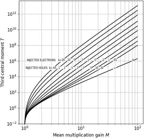
Figure 1 shows the behavior of the third central moment $T$ of the multiplication gain distribution $\mathcal{M}$ as a function of the mean value $M$ for different values of the ratio between hole and electron ionization coefficient $k$. Curves labeled with “injected electrons” correspond to $M(w)$ and $T(w)$ in Equation 49, whereas curves labeled with “injected holes” correspond to $M(0)$, converted from $M(w)$ using Equation 12, and $T(0)$ in Equation 48. The third central moment is equal to 0 in correspondence of the minimum mean multiplication gain $M=1$ and is always a positive quantity, indicating that the gain distribution is right-skewed, i.e., its tail is more pronounced on the right-hand side of the mean toward higher gain values.

Figure 1

Figure 1. Third central moment of the multiplication gain distribution as a function of the mean value for several values of the ratio $k$. Curves labeled with “injected electrons” correspond to $M(w)$ and $T(w)$ in Equation 49, while curves labeled with “injected holes” correspond to $M(0)$, converted from $M(w)$ using Equation 12 and $T(0)$ in Equation 48.

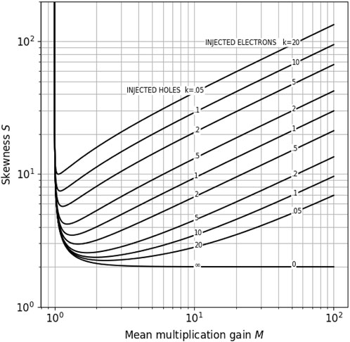
Figure 2 shows the skewness $S$ of the multiplication gain distribution $\mathcal{M}$, computed according to Equation 34, as a function of the mean value $M$ and for different values of $k$. The curve labeling has the same meaning, as shown in Figure 1. Salient characteristics of the skewness are i) as $M$ tends to 1, $S$ tends to infinity; ii) $S$ has a global minimum at positions slightly above the unity gain, depending on the value of $k$; and iii) $S$ is always higher than 2, which is typically indicated as a threshold for a distribution to be considered significantly skewed [24].

Figure 2

Figure 2. Skewness of the multiplication gain distribution, computed using Equation 34, as a function of the mean value and for several values of the ratio $k$. The labeling has the same meaning, as shown in Figure 1.

Figure 3 shows, as an example, the skewness $S$ of the distribution of the total signal $\mathcal{P}$, resulting from the interaction, assumed point-like, of an ionizing particle with a silicon avalanche diode at position $x=w$, which corresponds to the “injected electron” case. The energy $E_0$ of the impinging particle is in the range 1 eV–1 keV, and the mean multiplication gain $M$ is in the range 1–1,000. The third central moment of the total signal $\mathcal{P}$ was computed with Equation 59, using Equations 60, 61. The pair creation energy is $ϵ=$ 3.61 eV, the Fano factor is $f=$ 0.125, and the ionization coefficient ratio is $k=$ 0.33. The plot includes skewness values of 0.5, indicative threshold of a mildly skewed distribution, and 2, indicative threshold of a highly skewed distribution, for reference. As shown in Figure 2, increasing values of mean multiplication gain lead to increased skewness, whereas increasing values of initial particle energy lead to decreased skewness as a consequence of the central limit theorem.

Figure 3

Figure 3. Skewness of the distribution of the total signal $\mathcal{P}$ following the point-like interaction of an ionizing particle of energy $E_0$ with a silicon avalanche diode at position $x=w$ (corresponding to the “injected electron” case), exhibiting a mean multiplication gain $M$ and $k=$ 0.33. Skewness values of 0.5 indicate a mildly skewed distribution and 2 indicate a highly skewed distribution, which are shown for reference.

4 Conclusion

We derived exact analytical expressions for the variance, the third central moment, and the skewness of the multiplication gain in uniform avalanche structures as a function of the starting position of the electron–hole pair generating the avalanche. The expressions were obtained by solving integral equations based on the property of additivity of the central statistical moments of the sum of random variables and moment composition rules of the random sum. The assumptions include Poissonianity and locality of the ionization process. The model is valid for arbitrary values of electron and hole ionization coefficients $\alpha$ and $\beta$, respectively, as functions of the space coordinate. Although the variance is already known from its relationship with the excess noise in current fluctuations in stationary conditions via Milatz’s theorem, this study, provides an alternative, perhaps more physically intuitive, derivation.

Expressions are then provided for the particular case where the ionization coefficients are related by a constant ratio $k=\beta /\alpha$. In this context, it is found that the third central moment increases asymptotically with the fifth power of the mean multiplication gain and that the skewness is always positive and greater than 2, which is typically indicated as a threshold for a distribution to be considered significantly skewed.

The impact of the first three central moments of the multiplication gain distribution on spectral measurements of ionizing radiation was also evaluated through the use of the composition rules for a random sum. In this framework, we adopted the COM–Poisson distribution, a generalization of the Poisson distribution which takes into account the under-dispersion effect parameterized by the Fano factor as a description of the distribution of the initial number of photo-generated electron–hole pairs.

Data availability statement

The raw data supporting the conclusions of this article will be made available by the authors, without undue reservation.

Author contributions

PZ: writing–original draft and writing–review and editing.

Funding

The author(s) declare that no financial support was received for the research, authorship, and/or publication of this article.

Conflict of interest

Author PZ was employed by DECTRIS Ltd.

Publisher’s note

All claims expressed in this article are solely those of the authors and do not necessarily represent those of their affiliated organizations, or those of the publisher, the editors, and the reviewers. Any product that may be evaluated in this article, or claim that may be made by its manufacturer, is not guaranteed or endorsed by the publisher.

Footnotes

¹Please refer to [16] for a critical review of this approximation to the purpose of the excess noise factor in the noise spectral density of current fluctuations.

²The property of additivity of the central moments of the sum independent stochastic variable holds up to the third degree, so the method presented in the text cannot be extended to higher moments.

³For example, in silicon, assuming $ϵ=$ 3.61 eV and $f=$ 0.125, an error below 10% is obtained for $E_0>$ 60 eV.

References

1. Maes W, De Meyer K, Van Overstraeten R. Impact ionization in silicon: a review and update. Solid-State Electronics (1990) 33(6):705–18. doi:10.1016/0038-1101(90)90183-F

CrossRef Full Text | Google Scholar

2. Tager AS. Current fluctuations in a semiconductor under the conditions of impact ionization and avalanche breakdown. Fiz Tverd Tela (1964) 6:2418–2427.

Google Scholar

3. McIntyre RJ. Multiplication noise in uniform avalanche diodes. IEEE Transaction Electron Devices (1966) 13:164–8. doi:10.1109/T-ED.1966.15651

CrossRef Full Text | Google Scholar

4. Ramirez DA, Hayat MM, Huntington AS, Williams GM. Non-local model for the spatial distribution of impact ionization events in avalanche photodiodes. IEEE Photon Technology Lett (2014) 26(1):25–8. doi:10.1109/LPT.2013.2289974

CrossRef Full Text | Google Scholar

5. Van Vliet KM, Rucker LM. Theory of carrier multiplication and noise in avalanche devices—Part I: one-carrier processes. IEEE Transaction Electron Devices (1979) 26(5):746–51. doi:10.1109/T-ED.1979.19489

CrossRef Full Text | Google Scholar

6. Van Vliet KM, Friedmann A, Rucker LM. Theory of carrier multiplication and noise in avalanche devices - Part II: two-carrier processes. IEEE Transaction Electron Devices (1979) 26(5):752–64. doi:10.1109/T-ED.1979.19490

CrossRef Full Text | Google Scholar

7. Burgess RE. Some topics in the fluctuations of photo-processes in solids. J Phys Chem Sol (1961) 22:371–7. doi:10.1016/0022-3697(61)90284-0

CrossRef Full Text | Google Scholar

8. Milatz JMW. Nederl. Tijdschrift voor Natuurk. Phys. (1941) 8:19.

9. MacDonald DKC. Spontaneous fluctuations. Rep Prog Phys (1948) 12:56–81. doi:10.1088/0034-4885/12/1/304

CrossRef Full Text | Google Scholar

10. Van Vliet KM, Rucker LM. Noise associated with reduction, multiplication and branching processes. Physica (1979) 95A:117–40. doi:10.1016/0378-4371(79)90046-3

CrossRef Full Text | Google Scholar

11. Van Vliet KM. MacDonald’s theorem and Milatz’s theorem for multivariate stochastic processes. Physica (1977) 86A:130–6. doi:10.1016/0378-4371(77)90066-8

CrossRef Full Text | Google Scholar

12. Tan CH, Gomes RB, David JPR, Barnett AM, Bassford DJ, Lees JE, et al. Avalanche gain and energy resolution of semiconductor X-ray detectors. IEEE Transaction Electron Devices (2011) 58(6):1696–1701. doi:10.1109/TED.2011.2121915

CrossRef Full Text | Google Scholar

13. Vinogradov S. Feasibility of skewness-based characterization of SiPMs with unresolved spectra. Nucl Inst. Methods Phys Res A (2023) 1049:168028. doi:10.1016/j.nima.2023.168028

CrossRef Full Text | Google Scholar

14. Gabelli J, Reulet B. Full counting statistics of avalanche transport: an experiment. Phys Rev (2009) B 80:161203. doi:10.1103/PhysRevB.80.161203

CrossRef Full Text | Google Scholar

15. Van Brandt L, Vercauteren R, Enriquez DH, André N, Kilchytska V, Flandre D, et al. Variance and skewness of current fluctuations experimentally evidenced in single-photon avalanche diodes. In: 2023 International Conference on Noise and Fluctuations (ICNF); 17-20 October 2023; Grenoble, France.

Google Scholar

16. McIntyre RJ. The distribution of gains in uniformly multiplying avalanche photodiodes: theory. IEEE Transaction Electron Devices (1972) 19:703–13. doi:10.1109/T-ED.1972.17485

CrossRef Full Text | Google Scholar

17. Balaban P, Fleischer PE, Zucker H. The probability distribution of gains in avalanche photodiodes. IEEE Transaction Electron Devices (1976) 23:1189–90. doi:10.1109/T-ED.1976.18570

CrossRef Full Text | Google Scholar

18. Chakraborti NB, Rakshit S. Generation function in uniformly multiplying avalanche diode. IEEE Transaction Electron Devices (1984) 31:1346–7. doi:10.1109/T-ED.1984.21713

CrossRef Full Text | Google Scholar

19. Pilotto A, Antonelli M, Arfelli F, Biasiol G, Cautero G, Cautero M, et al. Modeling approaches for gain, noise and time response of avalanche photodiodes for X-rays detection. Front Phys (2022) 10:944206. doi:10.3389/fphy.2022.944206

CrossRef Full Text | Google Scholar

20. Giacomini G. LGAD-based silicon sensors for 4D detectors. Sensors (2023) 23:2132. doi:10.3390/s23042132

PubMed Abstract | CrossRef Full Text | Google Scholar

21. Hinger V, Barten R, Baruffaldi F, Bergamaschi A, Borghi G, Boscardin M, et al. Resolving soft X-ray photons with a high-rate hybrid pixel detector. Front Phys (2024) 12:1352134. doi:10.3389/fphy.2024.1352134

CrossRef Full Text | Google Scholar

22. Durnford D, Arnaud Q, Gerbier G. Novel approach to assess the impact of the Fano factor on the sensitivity of low-mass dark matter experiments. Phys Rev D (2018) 98:103013. doi:10.1103/PhysRevD.98.103013

CrossRef Full Text | Google Scholar

23. Gaunt RE, Iyengar S, Olde Daalhuis AB, Simsek B. An asymptotic expansion for the normalizing constant of the Conway–Maxwell–Poisson distribution. Ann Inst Stat Mathematics (2019) 71:163–80. doi:10.1007/s10463-017-0629-6

CrossRef Full Text | Google Scholar

24. Hair J, Black WC, Babin BJ, Anderson RE. Multivariate data analysis. 7th ed. Upper Saddle River, New Jersey: Pearson Educational International (2010).

Google Scholar

Appendix

Let $k\in \{\mathrm{0,1,2},\dots \}$ be a random variable, and let ${\{X_i\}}_{i=0}^{\infty }$ be independent identically random variables that are independent of $k$. The random variable $Y_k={\sum }_{i=0}^k{X}_i$ is called a random sum.

1 Mean value of a random sum

The mean value of the random sum $\mathbb{E}[Y_k]$ is straightforwardly

$\mathbb{E}\left[Y_k\right]=\mathbb{E}\left[X_0\right]\mathbb{E}\left[k\right].(\mathrm{B1})$

2 Variance of a random sum

The variance of a random sum $\mathbb{V}[Y_k]$ is [7, 10]

$\mathbb{V}\left[Y_k\right]=\mathbb{V}\left[X_0\right]\mathbb{E}\left[k\right]+\mathbb{E}{\left[X_0\right]}^2\mathbb{V}\left[k\right].(\mathrm{B2})$

3 Third central moment of a random sum

The third central moment of a random sum $\mathbb{T}[Y_k]$ is

$\mathbb{T}\left[Y_k\right]=\mathbb{E}\left[k\right]\mathbb{T}\left[X_0\right]+\mathbb{E}{\left[X_0\right]}^3\mathbb{T}\left[k\right]+3\mathbb{E}\left[X_0\right]\mathbb{V}\left[X_0\right]\mathbb{V}\left[k\right].(\mathrm{B3})$

Proof

The third central moment $\mathbb{T}$ of any random variable $X$ is

$\mathbb{T}\left[X\right]=\mathbb{E}\left[{\left(X-\mathbb{E}\left[X\right]\right)}^3\right],(\mathrm{B4})$

$=\mathbb{E}\left[X^3\right]-3\mathbb{E}\left[X\right]\mathbb{V}\left[X\right]-\mathbb{E}{\left[X\right]}^3,(\mathrm{B5})$

which, in our case, means

$\mathbb{T}\left[Y_k\right]=\mathbb{E}\left[Y_k^3\right]-3\mathbb{E}\left[Y_k\right]\mathbb{V}\left[Y_k\right]-\mathbb{E}{\left[Y_k\right]}^3.(\mathrm{B6})$

By applying the theorem of total moment on a random sum, we can write

$\mathbb{E}\left[Y_k^3\right]={\displaystyle \sum _{i=0}^{\infty }}\mathbb{E}\left[Y_i^3|k=i\right]={\displaystyle \sum _{i=0}^{\infty }}\mathbb{E}\left[Y_i^3\right]\mathrm{P}\mathrm{r}\left(k=i\right).(\mathrm{B7})$

By inverting Equation B6, we know that for any $Y_i$, the following holds:

$\mathbb{E}\left[Y_i^3\right]=\mathbb{T}\left[Y_i\right]+3\mathbb{E}\left[Y_i\right]\mathbb{V}\left[Y_i\right]+\mathbb{E}{\left[Y_i\right]}^3,(\mathrm{B8})$

and from basic statistics, we also know that

$\mathbb{E}\left[Y_i\right]=i\mathbb{E}\left[X_0\right],(\mathrm{B9})$

$\mathbb{V}\left[Y_i\right]=i\mathbb{V}\left[X_0\right],(\mathrm{B10})$

$\mathbb{T}\left[Y_i\right]=i\mathbb{T}\left[X_0\right],(\mathrm{B11})$

so that Equation B8 becomes

$\mathbb{E}\left[Y_i^3\right]=i\mathbb{T}\left[X_0\right]+3i^2\mathbb{E}\left[X_0\right]\mathbb{V}\left[X_0\right]+i^3\mathbb{E}\left[X_0\right],(\mathrm{B12})$

and therefore, Equation B7 can be written as

$\mathbb{E}\left[Y_k^3\right]={\displaystyle \sum _{i=0}^{\infty }}\left[i\mathbb{T}\left[X_0\right]+3i^2\mathbb{E}\left[X_0\right]\mathbb{V}\left[X_0\right]+i^3\mathbb{E}{\left[X_0\right]}^3\right]\mathrm{P}\mathrm{r}\left(k=i\right),(\mathrm{B13})$

$=\mathbb{E}\left[k\right]\mathbb{T}\left[X_0\right]+3\mathbb{E}\left[k^2\right]\mathbb{E}\left[X_0\right]\mathbb{V}\left[X_0\right]+\mathbb{E}\left[k^3\right]\mathbb{E}{\left[X_0\right]}^3.(\mathrm{B14})$

By substituting Equation B14 into Equation B6 and obtaining the mean value of a random sum from Equation B1 and the variance of a random sum from Equation B2, we get

$\mathbb{T}\left[Y_k\right]=\mathbb{E}\left[Y_k^3\right]-3\mathbb{E}\left[Y_k\right]\mathbb{V}\left[Y_k\right]-\mathbb{E}{\left[Y_k\right]}^3,(\mathrm{B15})$

$\begin{array}{ll}\hfill & =\mathbb{E}\left[k\right]\mathbb{T}\left[X_0\right]+3\mathbb{E}\left[k^2\right]\mathbb{E}\left[X_0\right]\mathbb{V}\left[X_0\right]+\mathbb{E}\left[k^3\right]\mathbb{E}{\left[X_0\right]}^3\hfill \\ \hfill & -3\mathbb{E}\left[k\right]\mathbb{E}\left[X_0\right]\left(\mathbb{E}\left[k\right]\mathbb{V}\left[X_0\right]+\mathbb{E}{\left[X_0\right]}^2\mathbb{V}\left[k\right]\right)-\mathbb{E}{\left[k\right]}^3\mathbb{E}{\left[X_0\right]}^3,\hfill \end{array}(\mathrm{B16})$

$=\mathbb{E}\left[k\right]\mathbb{T}\left[X_0\right]+\mathbb{E}{\left[X_0\right]}^3\left(\mathbb{E}\left[k^3\right]-3\mathbb{E}\left[k\right]\mathbb{V}\left[k\right]-\mathbb{E}{\left[k\right]}^3\right)+3\mathbb{E}\left[X_0\right]\mathbb{V}\left[X_0\right]\left(\mathbb{E}\left[k^2\right]-\mathbb{E}{\left[k\right]}^2\right),(\mathrm{B17})$

$=\mathbb{E}\left[k\right]\mathbb{T}\left[X_0\right]+\mathbb{E}{\left[X_0\right]}^3\mathbb{T}\left[k\right]+3\mathbb{E}\left[X_0\right]\mathbb{V}\left[X_0\right]\mathbb{V}\left[k\right].(\mathrm{B18})$