Fast and precise dose estimation for very high energy electron radiotherapy with graph neural networks

Introduction: External beam radiotherapy (RT) is one of the most common treatments against cancer, with photon-based RT and particle therapy being commonly employed modalities. Very high energy electrons (VHEE) have emerged as promising candidates for novel treatments, particularly in exploiting the FLASH effect, offering potential advantages over traditional modalities.

Methods: This paper introduces a Deep Learning model based on graph convolutional networks to determine dose distributions of therapeutic VHEE beams in patient tissues. The model emulates Monte Carlo (MC) simulated doses within a cylindrical volume around the beam, enabling high spatial resolution dose calculation along the beamline while managing memory constraints.

Results: Trained on diverse beam orientations and energies, the model exhibits strong generalization to unseen configurations, achieving high accuracy metrics, including a $\delta$-index 3% passing rate of 99.8% and average relative error $<$1% in integrated dose profiles compared to MC simulations.

Discussion: Notably, the model offers three to six orders of magnitude increased speed over full MC simulations and fast MC codes, generating dose distributions in milliseconds on a single GPU. This speed could enable direct integration into treatment planning optimization algorithms and leverage the model’s differentiability for exact gradient computation.

1 Introduction

In the treatment of cancer for deep-seated tumors, external beam radiotherapy (RT) is recognized as one of the most effective and commonly employed therapies [1]. Various types of radiation have been explored, with X-ray radiotherapy being the most commonly used, while a smaller portion of patients undergo particle therapy (PT) utilizing protons or heavier ions. Electrons, due to their unique interaction properties with matter, offer potential advantages over photon RT and PT, especially for specific irradiation modalities [2, 3]. For example, electrons possess an advantageous attribute since they can be easily stirred by a magnetic field, providing great flexibility in selecting the entry angles of the radiation beams. Very high-energy electrons (VHEE) in the 60–120 MeV range have been investigated for treating deep-seated tumors, demonstrating comparable performance to volumetric modulated arc therapy (VMAT) [4] and proton irradiation, albeit with complexities and cost considerations [5, 6]. Technological advances, such as compact and cost-effective C-band accelerating structures, now enable the feasible production of high-energy electron fields, potentially making VHEE therapy more accessible for clinical use [7].

Finally, there has been growing interest in the exploration of high-dose-rate therapies, with electron FLASH therapy standing out as a possible revolutionary treatment [8]. FLASH-RT is a novel approach that promises an ultra-fast delivery of radiation (less than 200 milliseconds per treatment) with pulses featuring an ultra-high dose rate ($>$ 40 Gy/s). This makes FLASH-RT approximately 400 times faster than traditional radiotherapy, with a dose rate several orders of magnitude higher than the traditional rate (approximately 0.5 Gy/min). FLASH-RT derives its name from the “FLASH effect” a biological phenomenon where irradiation at ultra-high dose rates exhibits a superior ability to spare healthy tissues while maintaining its effectiveness against tumors [9–11].

The prime candidates for fully exploiting the potential of this effect are believed to be electrons, specifically VHEE, for the treatment of deep-seated tumors [2, 12]. Currently, a treatment planning (TP) algorithm exploiting the electron beam possibilities is needed. The first step for a TP system is the estimation of the dose as a function of the beam parameters. The ongoing research in the field of TP for VHEE RT and electron FLASH-RT predominantly relies on Monte Carlo (MC) simulations or the development of fast MC simulations, such as FRED (Fast paRticle thErapy Dose evaluator) [12–14].

In this context, deep learning (DL) algorithms are a promising alternative to overcome current limitations, offering a dual benefit of speed and precision in dose estimation. These algorithms can be trained to replicate the output of MC simulations, enabling the fast generation of dose distribution maps with a precision comparable to MC. Moreover, the speed of DL models in generating these dose distributions and the differentiability of their output enable the development of a TP system based on them. Such a TP system could integrate them into the merit function and exploit gradient-based optimization algorithms for plan optimization.

Recently, an increasing number of studies on the application of DL techniques to dose estimation and treatment planning has emerged [15]. The majority of these studies concentrate on clinically established treatments for which extensive datasets from past patients are readily available. Moreover, only a limited number address the DL emulation of dose distributions for individual beams or fields [16, 17], while the majority of these efforts aim to replicate entire treatment plans based on historical records [18, 19]. Although it has been shown that DL models can effectively reproduce the dose distributions, it is important to note that the accuracy of DL models is intrinsically constrained by the precision of the algorithms that they are trained to emulate. However, these are often the deterministic algorithms used in the optimization of most current treatment plans [18, 19]. Conversely, we propose that the true advantage of employing DL lies in emulating MC simulations, which, although substantially more accurate than deterministic algorithms, are currently too slow for practical clinical use. This approach can potentially enhance both treatment efficiency and quality.

Few studies have explored the feasibility of reproducing MC-simulated dose distributions [20, 21], and these are primarily focused on novel radiotherapy treatments where deterministic algorithms are not applicable. Finally, no DL-based solution has yet been developed or applied for VHEE RT dose estimation.

We thus introduce a DL model designed to replicate MC-simulated dose distributions for therapeutic VHEE beams in patient tissues. Our strategy involves considering a voxelized cylindrical volume around the beam, enabling us to predict the dose at varying spatial resolutions. This approach minimizes the model’s memory requirements while maintaining high accuracy in the most relevant regions. The model is trained to take as input the beam’s energy and the densities of organs inside the cylinder around the beam and delivers an accurate and ultra-fast (0.02 s on CPU) estimate of the dose distribution within the cylinder.

This paper is organized as follows. Section 2 describes in detail the MC simulations used to build the dataset to train our DL model along with the description of the model itself. Section 3 presents the metrics used to evaluate our model and summarize the main results of our work. Finally, Section 4 is dedicated to final discussion and conclusions.

2 Materials and methods

The proposed DL model is trained to estimate the dose distribution in a cylindrical volume with the symmetry axis aligned with the beam. It outputs a 3D cylindrical dose map which uses as input the densities in such a cylinder and the beam energy.

2.1 Dataset

2.1.1 Monte Carlo simulation

The dataset used to train, validate, and test the proposed DL model was built running a set of MC simulations using the Geant4 toolkit (version 11.1.1) [22–24]. Geant4 is the most used toolkit for developing radiation matter MC simulations, being regularly validated also for medical applications [25]. Each element of the dataset is a different simulation in which an electron beam of varying energy and orientation simulates an incident on a patient’s head and neck CT scan.

The CT scan used in this study contains the head of a patient with a meningioma (hereafter M1) treated at the Trento Particle Therapy Center. We decided to use the M1 patient CT scan because it has been used in a recent publication to compare treatment plans delivered with VHEE FLASH RT, IMRT, and Proton therapy [14]. In future, we plan to compare a DL generated treatment plan with that produced by currently available techniques. The CT scan was composed of 260 slices 1 mm thick. Each slice was composed of $512\times 512$ pixels with a side length of 0.6015626 mm. The CT scan was imported as the detector geometry in a Geant4 simulation based on the ICRP110 Human Phantoms Advanced Example [26].

Each voxel was assigned a material and a nominal density based on its Hounsfield unit (HU) value. Firstly, depending on the binning on HU values reported in Table 1, materials were assigned to each voxel. In particular, on the right side of Table 1 the upper bounds of the material binning were reported so that voxels with HUs $-820$ were assigned to the material “Air”, voxels with HU between $-820$ and 39 were assigned the material “Soft Tissue”, and so on. The material list is that used for the Geant4 DICOM Digital Head in the DICOM example [27]. HU boundary values between different organs were computed based on the data in [27] where HU mean and standard deviation values were reported for each tissue. Boundaries are computed as the intersection points between the Gaussian distributions with those mean and standard deviation values. The upper bound for the air was set manually to $-820$. In Geant4, a material is defined by an atomic composition and a density value. To avoid the definition of a large number of materials (one for each density value), we created a sub-binning for each material with bin width equal to 50 HU. Using the calibration curve used for the treatment planning of M1 [14] (reported in Table 2), a nominal density was then assigned to each voxel. Finally, nominal densities were averaged, so that each voxel of a certain material’s sub-bin had the average density of the voxels assigned to that sub-bin. As a result, there was univocal correspondence between HU sub-bin ranges, materials, and densities.

Table 1

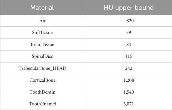
Table 1. Materials’ table. Left column: list of materials used in the MC simulation, based on that used in [27]. Right column: upper bound of the material binning is reported so that all voxels with HU less than $-820$ are assigned to the material “Air”, all voxels with HU between $-820$ and 39 are assigned the material “Soft Tissue”, and so on.

Table 2

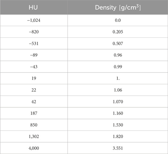
Table 2. Calibration curve which rules the conversion between HU and density, for the patient M1 [14]. The calibration curve was used to assign each voxel of the CT scan a nominal density value.

Using this geometry setting, therapeutic very high energy electron (VHEE) beams were directed towards the center of the CT scan. Each beam was modeled as a Gaussian pencil-beam with a full width at half maximum (FWHM) of 0.5 cm whose source lies on a 30-cm-radius sphere centered in the CT scan center. To collect dose data, we used a cylindrical scorer with the $z$ axis aligned with the beam. The scorer comprised 100 voxels of 4 mm length along the $z$ axis, 20 voxels of 4 mm length along the $r$ axis, and 25 voxels along the theta axis, so that the inner voxels had an angular length of $\sim 1$ mm, while the outer ones had an angular length of $\sim 2$ cm.

Using a cylindrical scorer has two main advantages. The first is that it is more precise near the beam line, where most of the dose is deposited. The second advantage regards the exemplification of the DL emulation problem. We required the DL model to reproduce the dose in the cylinder around the beam so that we did not have to account for a direct dependence on the beam orientation. Because the beam distribution was fixed, the dose only depended on the beam energy and the densities of the tissues in the cylindrical region around the beam. On the left of Figure 1, we present a two-dimensional schematic representation of cylindrical voxels superimposed on a regular grid. Depending on the grid spacing and cylinder voxelization, the cylindrical scorer can have an increased resolution near the beamline. In the same figure, the central and right panels show front and lateral slices of the CT scan, respectively. The blue regions correspond to the intersection with a cylinder whose axis is represented by the light blue line in the right panel.

Figure 1

Figure 1. Cylindrical approximation. Left: 2D schematic drawing of cylindrical voxels superimposed on a regular grid. Center and right panels: front and lateral sections of the CT scan. The intersection between the CT scan and a cylinder is highlighted in blue. Right panel: the cylinder axis, which coincides with the beam line, is displayed as a light blue line.

It is worth noting that the actual tracing in the simulation was done considering the CT voxels, and only the scoring was done in the cylindrical voxels.

Using this setting, we generated a dataset of 10.000 examples with low statistics (10.000 primaries per beam, average 20% statistical uncertainty) to train, validate, and test the DL model. Each example contained the dose of a monochromatic electron beam inside the cylindrical scorer. The beam energy was uniformly sampled between 70 and 130 MeV. The two angular values defining the orientation of the beams $\theta$ and $\varphi$ were sampled uniformly as integers respectively of 0–180° and 0–360°.

Our dataset was built to simulate conventional VHEE beams, and our DL model was trained to reproduce such simulations. It is possible to account for the FLASH effect after the conventional dose calculation using the FLASH modifying factor (FMF), as in [14]. The FMF, defined in [28], is the ratio of doses that need to be administered at conventional and ultra-high dose rates to achieve the same effect for a given biological system. Thus, by multiplying the simulated absorbed dose by the FMF, it is possible to account for the organs at risk induced by the FLASH effect [14]. Such a computation was performed after the treatment plan optimization and thus was not an object of this study.

2.1.2 Density interpolation

As already mentioned, we sought to train the DL algorithm to produce the dose map in a density map with the same mesh of the input.

Therefore, for each example, we computed the density values in the cylindrical voxels interpolating the densities we assigned to the CT scan voxels. To obtain a reliable estimate of the density, we sampled $N$ random 3D points inside each cylindrical voxel. We then computed the fraction of such points that fall in each of the CT voxels, to which we refer as $N_i$, $i\in \{1,N_{\mathit{CTvox}}\}$. The density associated with a cylindrical voxel $j{\rho }^j$ is then the average of the density in the CT voxels weighted by the values {$N_i$} (Equation 1):

${\rho }^j=\frac{{\sum }_i{N}_i{\rho }_i}{N}.(1)$

For large $N$, this expression converges to the average weighted with intersection volumes (Equation 2):

${\rho }^j=\frac{{\sum }_i{v}_i^j{\rho }_i}{V_j},(2)$

where $V_j$ is the volume of the cylindrical voxel $j$, while $v_i^j$ is the volume of the intersection between the cylindrical voxel $j$ and the CT voxel $i$. We chose $N$ to be equal to 100 in order to obtain a satisfactory estimate in a contained computing time. The study we performed for choosing the most suitable number of sampling points can be found in the Supplementary Material.

The cylindrical density maps represent the input to our DL model, along with the information about the beam energy.

2.2 Deep learning model

The DL model developed in this work is based on graph neural networks and has a U-net structure. A U-net [29] is a two-dimensional fully convolutional neural network that is widely used in medical applications. Its encoder–decoder architecture, combined with skip connections, enables efficient modeling of hierarchical features while mitigating the issue of vanishing gradients. To account for the geometric structure of our data, we replaced traditional with graph convolutions. Such a model represents an improvement over the already published recursive nearest neighbors (ReNN) graph variational auto encoder [30], which we proved to be effective in predicting dose distributions in homogeneous and simple in-homogeneous materials. Finally, we compared such a model to a 3D U-net on a dose prediction task on standard grid-like data presented in [21], finding comparable or superior performance [31].

The model is composed of three modules: the encoder, the embedder, and the decoder. The encoder takes input from the density cylindrical graphs $\rho$, each with 50.000 nodes. Data are processed through six GraphConv layers with an increasing number of output channels: 32, 64, 128, 256, 256, 256 followed by rectified linear unit activation (ReLu) functions. In the GraphConv layer, the new node features $x^{\prime }$ are a linear combination between their old features $x$ and a weighted mean of their neighbors’ features (Equation 3):

$x_i^{\prime }=ReLu\left(W_1{x}_i+W_2\frac{1}{|N\left(i\right)|}{\displaystyle \sum _{j\in N\left(i\right)}}{e}_{ij}{x}_j\right).(3)$

The edge features $e_{ij}$ represent the weight of the link between nodes $i$ and $j$; in our model, they are learnable parameters of the network. Between the convolutive layers, we used ReNN-Pool [30]. This pooling technique allows the graph to reduce dimensionality, dropping a consistent number of nodes but always assuring a unique connected graph, creating new links between far nodes regularly and efficiently. After five pooling operations, the output of the encoder consisted of a small connected graph with 33 nodes.

The embedder is a two-layer multilayer perceptron which takes input from the energy of the beam $E$ and outputs a feature map with the dimensionality of the number of nodes in the smallest graph representation—33 nodes. The output of the encoder and the embedder are then summed.

The decoder applies five GraphConv layers with a decreasing number of output channels: 256, 128, 64, 32, 1. Each GrapConv layer is followed by a ReLu activation except the last, which is followed by a sigmoid activation function. Before each convolutive layer, ReNN-UnPool is applied to retrieve the original graph dimensionality and to allow skip connection between the encoder and the decoder. Indeed, each decoder layer takes as input the sum of the unpooled output of the previous layer and the partial output from the skip connection coming from the encoder.

Figure 2 presents a schematic representation of the model architecture, including only two pooling layers for simplicity.

Figure 2

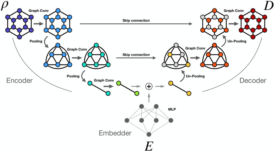
Figure 2. ReNN GU-Net. Simplified scheme of the ReNN GU-Net with two pooling layers. Density information $\rho$ in the form of a 3D graph is processed by the model through the encoder. The energy of the beam $E$ is processed by the embedder and then added to the encoder output. The resulting graph is processed by the decoder to retrieve the original graph dimensionality and to predict the dose distribution $D$.

3 Results and discussion

We divided our 10.000 example dataset between train, validation, and test sets. The examples selected for the test set are 275 and satisfy these conditions:

$•$ Beam energy $E\in [\mathrm{60,70}]\cup [\mathrm{80,90}]$ MeV,

$•$ Angle $\theta \in [\mathrm{45,75}]\cup [\mathrm{105,135}]$ degree,

$•$ Angle $\varphi \in [\mathrm{75,105}]\cup [\mathrm{165,195}]\cup [\mathrm{255,285}]$ degree.

The rest of the dataset was split between train and validation sets with a 1/10 ratio, so that the training set contained 8,752 examples while the validation set contained 973. We chose this arrangement for the test set in order to put ReNN GU-Net under a strict test, testing its ability to interpolate between samples and generalize to unseen configurations from both the point of view of patient anatomy and the beam’s energy.

We also generated ten high statistical examples, whose Geant4 simulations were run using one million primaries per beam ($\times 100$ more particles than in train, validation, and test sets) with an average statistical uncertainty of 2%. These samples, whose energies and orientations lie in the ranges of the test set, were used for the final evaluation and plots.

After an extensive hyper-parameter optimization of the learning rate, convolutional filters, and model depth, we trained our final model with a learning rate of 0.005 and a batch dimension of 16, with the learning rate scheduler ReduceOnPlateau with a patience of 20 epochs. The model was trained using Binary Cross-Entropy loss. We stopped the training at the convergence of the validation loss after 104 epochs. The training was conducted on a Tesla V100 GPU and lasted approximately 4 h. The complete information about the hyper-parameter optimization can be found in the Supplementary Material.

In order to evaluate the results of our model, we considered four different metrics:

$•$ Mean absolute error (MAE): voxel-wise mean absolute error between MC and DL dose.

$•$ $\delta$-index: introduced by Mentzel [20] and inspired by the clinical $\gamma$-index [32]. It quantifies the voxel-wise absolute error difference between MC and DL doses normalized by the maximum dose. This measure gives less importance to regions in which the dose is low and thus are therapeutically less important. In particular, we consider the $\delta$-index 3% passing rate, which accounts for the percentage of voxels in which the $\delta$-index if less than 3%.

$•$ Mean relative error (MRE) on dose profiles. We compute the integrated dose profiles along the two cylindrical axes $z$ and $r$ and compute the MRE between the MC and DL predictions. We refer to these metrics as MRE $z$ and MRE $r$.

$•$ MRE on total dose. MRE computed on the full integral of the dose, which represents the total dose, computed with MC and DL. We refer to this measure as MRE $E$

We present the results for all metrics in Table 3 for the training, validation, testing, and evaluation sets. The MAE, expressed in micrograys ($\mu$Gy), is calculated considering the dose as deposited by a beam of $10^6$ electrons.

Table 3

Table 3. Dose results: we report the results for all metrics for training, validation, testing, and high-statistics evaluation set. Note that the best agreement is found for the evaluation set because, by construction, DL models produce a smooth approximation of the learned function.

The best agreement is observed on the high statistics examples of the evaluation set. Increasing the statistics in an MC simulation yields a reduction of the fluctuations with a consequent better estimate of the dose distribution. DL models, by construction, learn to interpolate smooth functions between the training samples. Models based on convolutional layers are particularly known for their smoothing effect on outputs. This effect is leveraged in de-noising tasks, also performed on MC simulations for radiation therapy [33], where a model is trained to suppress fluctuations in noisy images or distributions. We took advantage of this effect by training our DL model on low-statistics samples, which can be produced more quickly, testing it on clinically valid high-statistics MC samples. As shown in the results, the model learns to ignore the fluctuation and predict a good estimate of the dose distribution, comparable with the one generated by high statistics MC simulations.

All the metrics show good agreement between the MC simulated dose and the DL emulated one, with 99.8% of the voxels of the evaluation set examples exhibiting a $\delta$-index inferior to 3%.

In the top plots of Figure 3, we show the integrated dose profiles along the $z$ and $r$ axes of the cylinder for an example drawn from the high-statistics evaluation set with beam orientation defined by $\theta$ = 122° and $\varphi$ = 178°, and beam energy $E$ = 82.44 MeV. The dose profiles predicted by our ReNN GU-Net (in orange) agree with the MC simulated profiles (in blue), even on the boundaries between tissues with very different densities. The average density in $\text{g}/{\text{cm}}^3$ computed from the CT scan using a calibration curve, as explained in Section 2.2, is also shown for reference as a dashed gray line. The agreement between the two profiles is quantified in the bottom plots, where we report respectively the absolute difference between the profiles (Err) and the percentage relative error between the profiles (Rel Err) in blue dots. In both plots we also report the standard deviation of the MC simulation (gray band). The percentage relative error is computed directly between the two integrated profiles as follows (Equation 4):

$RE\left[\%\right]=\frac{D_{MC}^{\mathit{prof}}-D_{DL}^{\mathit{prof}}}{D_{MC}^{\mathit{prof}}}\times 100,(4)$

where $D_{MC}^{\mathit{prof}}$ and $D_{DL}^{\mathit{prof}}$ are respectively the dose profiles computed with a MC simulation and with our DL model. The relative error is mostly inferior to $2$% except from the tails of the distributions, where a lower amount of dose is deposited. These regions are typically those in which the standard deviation of the MC simulation is also higher due to the low statistics. Indeed, as is evident from the middle and bottom plots, the errors appear to be correlated with the MC standard deviation, and the absolute error rarely exceeds 0.1 mGy. It is worth noting that the tails of the dose distribution are subject to a large amount of uncertainty in the low-statistics training examples of over 50%. Therefore, a larger error in the DL prediction, but still coherent with the MC uncertainty, is expected.

Figure 3

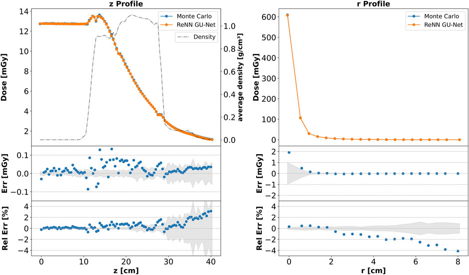
Figure 3. Integrated dose profiles. Top: comparison of dose profiles along the $z$ and $r$ axes of the cylinder, computed through MC simulation (blue) and our DL model (orange), showcasing an example from the high-statistics evaluation set. The average CT scan density, calculated from HU using a calibration curve, is indicated by a gray dashed line. Bottom: absolute error and percentage relative error between the dose profiles computed by MC and DL methods (blue dots) along with the MC standard deviation (gray band).

The agreement is not limited to the integrated profiles but also extends locally. In Figure 4, we present a plot similar to that in Figure 3, depicting the dose profiles along the $z$-axis. This computation is specifically for the central voxels, considering only one voxel along the $r$-axis and marginalizing over $\theta$. This accounts for the region in the highest proximity to the beam line with $r<4$ mm, where a large amount of dose is deposited—around $75$% of the total. Such a plot shows that the agreement between MC and DL dose profiles persists, also restricting our analysis in the core of the cylinder. Looking at the bottom plots, it is worth noting that the relative error is also clearly correlated in this case with the standard deviation of the MC simulation, and that DL and the MC curves are mostly consistent within a standard deviation.

Figure 4

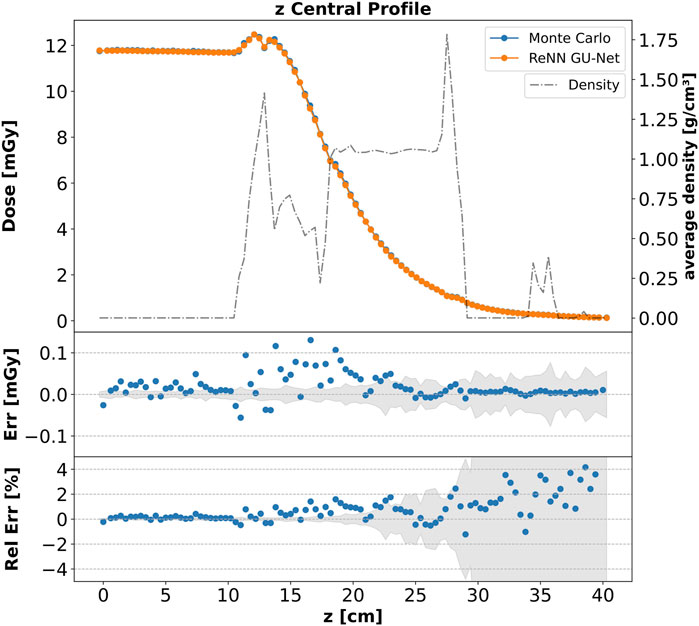
Figure 4. Core dose profile. Top: comparison of the dose $z$ profile computed for the core cylinder around the beam (with $r<4$ mm), using MC simulation (blue) and our DL model (orange), for an example from the high-statistics evaluation set. The average CT scan density, calculated from HU using a calibration curve, is indicated by a gray dashed line. Bottom: absolute error and percentage relative error between the dose profiles computed by MC and DL methods (blue dots) along with the MC standard deviation (gray band).

To show our model’s ability to generalize to different unseen beam energies and orientations, Figure 5 compares DL and MC computed core dose profiles for four additional examples from the evaluation set. Each panel’s title reports the two angles, $\theta$ and $\varphi$, that define the beam orientation, as well as the beam energy for the respective example. In all cases, discrepancies between DL and MC are mostly within the range of MC uncertainty.

Figure 5

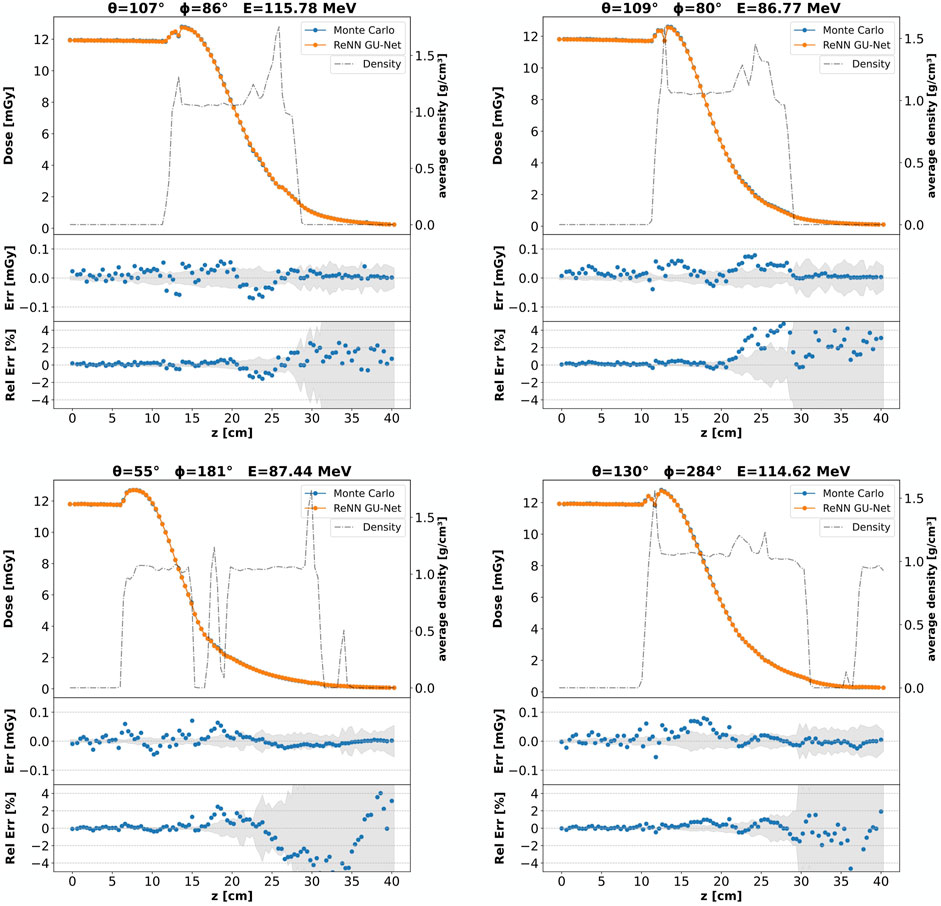
Figure 5. Core dose profiles: different beam configurations. Each panel corresponds to a different example from the evaluation set, featuring varying beam energies and orientations as indicated by the panel titles. For each panel, a comparison of the core dose $z$-profile computed using MC simulation (blue) and our DL model (orange) is shown, along with the average CT scan density represented by a gray dashed line. Below each profile: the absolute error and the percentage relative error between the dose profiles computed by the MC and DL methods (blue dots) are displayed, along with the MC standard deviation (gray band).

In Figure 6 we show a visual comparison between the CT scan (in the left panel), the MC simulated dose (central panel), and the DL emulated dose (right panel). These panels were extracted from our cylindrical structures considering two opposite sets of voxels in the $\theta$ dimension. In other words, these represent a horizontal slice taken from the cylinder, slicing it in one of the $z$-$r$ planes.

Figure 6

Figure 6. CT, Monte Carlo, and ReNN GU-Net. Image representation of a horizontal slice taken from the considered cylindrical volume around the beam. On the left panel is shown the CT scan, which is the input to our DL model. The MC simulated and DL predicted dose distributions are reported, respectively, on the central and right panels.

Moreover, we show in Figure 7 the $\delta$-index computed on the cylinder slice shown in Figure 6. $\delta$-index values are reported for all but the voxels which contain air. On a green-to-yellow scale, we report all the $\delta$-index values below 3%, while on a yellow-to-red scale the higher values (up to 3.8%) are drawn.

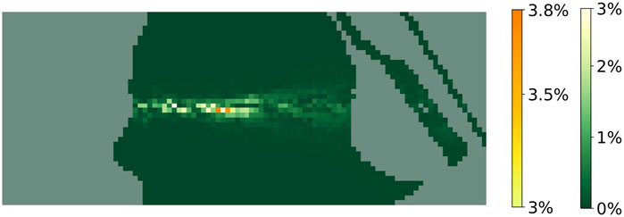
Figure 7

Figure 7. $\mathbf{\delta }$-index. Distribution of the $\delta$-index computed on the voxels of a slice of the cylinder around the beam. The green-to-yellow scale indicates values below 3%; yellow-to-red scale indicates higher values.

Finally, our DL model can significantly enhance speed in generating dose distributions. Currently, the available methods to compute VHEE dose maps are full MC simulations and fast MC codes such as FRED, which run on GPU. Our DL algorithm produces a dose map in approximately 0.02 s on a 16-core CPU (HP Z2 Tower G5 Workstation). A full MC simulation with Geant4 takes five orders of magnitude more time on the same machine. Moreover, running the DL model on GPU devices can further reduce the execution time. Generating a single example on a Nvidia Tesla V100 32G GPU takes approximately 7 milliseconds. If generating in batches, the execution time can be further reduced: generating a batch of 64 samples takes approximately 0.15 s, bringing the generation time of a single sample down to 2.3 milliseconds—roughly three orders of magnitude faster than FRED.

Although the DL dose engine presented shows promise in balancing accuracy and speed in dose computation, it is important to note some limitations. This study aims to demonstrate the feasibility and effectiveness of the cylindrical scoring method combined with an innovative GNN-based DL model for dose predictions. Although nearly 100% of the dose predictions achieve a $\delta$-index passing rate of 3% inspired by the clinical global $\gamma$-index, the current cylindrical voxel dimensions along $z$ and $r$ do not permit comparison at the required clinical spatial resolution. This comparison will be conducted in subsequent research, in which we plan to increase the cylinder’s resolution to meet, and even over-sample, in the core of the cylinder the clinically required spatial resolution. A larger cohort of patients will then be considered to test the model’s generalization ability. Given that the execution time of graph convolutional layers scales linearly with the number of nodes, reducing the resolution to 2 mm—increasing the nodes by a factor of 4—would still keep the total execution time below 10 ms.

4 Conclusion

The current study proposes a DL model to compute the dose distribution of a therapeutic VHEE beam in patient tissues. The model, based on graph convolutional networks, is trained to emulate the MC simulated dose inside a cylindrical volume around the beam. This approach allows us to compute the dose with high spatial resolution on the beamline, where most of the dose is deposited, while containing the model’s memory footprint. The model was trained on a set of examples comprising different beam orientations and energies, and it was tested on a different set. The test set has been realized using couples of beam orientation and energy not used to produce the train set to test model’s generalization capability. The model’s accuracy was measured using MAE and MRE on integrated dose profiles, and $\delta$-index. The results show that the model can generate dose distributions with a $\delta$-index 3% passing rate of 99.8%. Moreover, integrated dose profiles agree with MC simulations, with an average relative error less than 1%.

With respect to other current methods for calculating VHEE dose distributions—full MC simulations and FRED—our model provides an acceleration of several orders of magnitude. Indeed, it can generate dose distribution in milliseconds on a single GPU. The dose calculation is so fast that the DL model could be directly integrated into the merit function of an optimization algorithm for treatment planning. Moreover, taking advantage of the fact that the output of a DL model is differentiable with respect to the input, it would be possible to build a treatment planning optimization strategy based on exact gradient computation.

We plan to explore this possibility in future research aiming to build a treatment plan optimization algorithm which can fully exploit the benefits of DL dose generation.

Data availability statement

The raw data supporting the conclusions of this article will be made available by the authors, without undue reservation.

Ethics statement

Ethical approval was not required for the studies involving humans because this study uses the same patient data on a previously published paper in Frontiers in Physics: https://doi.org/10.3389/fphy.2023.1185598. As stated there: “Ethical review and approval was not required for the study on human participants, and written informed consent for participation was obtained.”

Author contributions

LA: conceptualization, data curation, formal analysis, investigation, methodology, resources, software, validation, visualization, writing–original draft, and writing–review and editing. BC: funding acquisition, supervision, writing–original draft, and writing–review and editing. AC: software, validation, writing–original draft, and writing–review and editing. AD: writing–original draft and writing–review and editing. GF: writing–original draft and writing–review and editing. StG: funding acquisition, resources, supervision, writing–original draft, and writing–review and editing. SuG: writing–review and editing, supervision, and writing–original draft. AM: data curation, writing–original draft, and writing–review and editing. FN: writing–original draft and writing–review and editing. JP: software, writing–original draft, and writing–review and editing. AS: funding acquisition, supervision, writing–original draft, and writing–review and editing. CM-T: conceptualization, formal analysis, funding acquisition, investigation, methodology, project administration, resources, software, supervision, validation, writing–original draft, and writing–review and editing.

Funding

The authors declare that financial support was received for the research, authorship, and/or publication of this article. This research was partially supported by PNRR MUR project PE0000013-FAIR. This research was partially funded by INFN National Scientific Committee 5 project FRIDA (Flash Radiotherapy with hIgh Dose-rate particle beAms).

Acknowledgments

The authors acknowledge the CINECA award under the ISCRA initiative for the availability of high-performance computing resources and support.

Conflict of interest

The authors declare that the research was conducted in the absence of any commercial or financial relationships that could be construed as a potential conflict of interest.

Publisher’s note

All claims expressed in this article are solely those of the authors and do not necessarily represent those of their affiliated organizations, or those of the publisher, the editors, and the reviewers. Any product that may be evaluated in this article, or claim that may be made by its manufacturer, is not guaranteed or endorsed by the publisher.

Supplementary material

The Supplementary Material for this article can be found online at: https://www.frontiersin.org/articles/10.3389/fphy.2024.1443306/full#supplementary-material

References

1. Delaney G, Jacob S, Featherstone C, Barton M. The role of radiotherapy in cancer treatment: estimating optimal utilization from a review of evidence-based clinical guidelines. Cancer (2005) 104:1129–37. doi:10.1002/cncr.21324

PubMed Abstract | CrossRef Full Text | Google Scholar

2. Schüler E, Eriksson K, Hynning E, Hancock SL, Hiniker SM, Bazalova-Carter M, et al. Very high-energy electron (VHEE) beams in radiation therapy; Treatment plan comparison between VHEE, VMAT, and PPBS. Med Phys (2017) 44:2544–55. doi:10.1002/mp.12233

PubMed Abstract | CrossRef Full Text | Google Scholar

3. Krim DE, Rrhioua A, Zerfaoui M, Bakari D. Monte Carlo modeling of focused very high energy electron beams as an innovative modality for radiotherapy application. Nucl Instrum Methods Phys Res A (2023) 1047:167785. doi:10.1016/j.nima.2022.167785

CrossRef Full Text | Google Scholar

4. Otto K. Volumetric modulated arc therapy: IMRT in a single gantry arc. Med Phys (2008) 35:310–7. doi:10.1118/1.2818738

PubMed Abstract | CrossRef Full Text | Google Scholar

5. Ronga MG, Cavallone M, Patriarca A, Leite AM, Loap P, Favaudon V, et al. Back to the future: very high-energy electrons (vhees) and their potential application in radiation therapy. Cancers (2021) 13:4942. doi:10.3390/cancers13194942

PubMed Abstract | CrossRef Full Text | Google Scholar

6. Maxim PG, Tantawi SG, Loo BW. PHASER: a platform for clinical translation of FLASH cancer radiotherapy. Radiother Oncol (2019) 139:28–33. doi:10.1016/j.radonc.2019.05.005

PubMed Abstract | CrossRef Full Text | Google Scholar

7. Giuliano L, Alesini D, Behtouei M, Bosco F, Carillo M, Cuttone G, et al. Preliminary studies of a compact VHEE linear accelerator system for FLASH radiotherapy. Geneva, Switzerland: JACOW Publishing (2021). 1229–32.

Google Scholar

8. Lin B, Gao F, Yang Y, Wu D, Zhang Y, Feng G, et al. FLASH radiotherapy: history and future. Front Oncol (2021) 11:644400. doi:10.3389/fonc.2021.644400

PubMed Abstract | CrossRef Full Text | Google Scholar

9. Favaudon V, Caplier L, Monceau V, Pouzoulet F, Sayarath M, Fouillade C, et al. Ultrahigh dose-rate FLASH irradiation increases the differential response between normal and tumor tissue in mice. Sci Transl Med (2014) 6:245ra93. doi:10.1126/scitranslmed.3008973

PubMed Abstract | CrossRef Full Text | Google Scholar

10. Vozenin MC, De Fornel P, Petersson K, Favaudon V, Jaccard M, Germond JF, et al. The advantage of FLASH radiotherapy confirmed in mini-pig and cat-cancer patients. Clin Cancer Res (2019) 25:35–42. doi:10.1158/1078-0432.ccr-17-3375

PubMed Abstract | CrossRef Full Text | Google Scholar

11. Bourhis J, Sozzi WJ, Jorge PG, Gaide O, Bailat C, Duclos F, et al. Treatment of a first patient with FLASH-radiotherapy. Radiother Oncol (2019) 139:18–22. doi:10.1016/j.radonc.2019.06.019

PubMed Abstract | CrossRef Full Text | Google Scholar

12. Sarti A, De Maria P, Battistoni G, De Simoni M, Di Felice C, Dong Y, et al. Deep seated tumour treatments with electrons of high energy delivered at FLASH rates: the example of prostate cancer. Front Oncol (2021) 11:777852. doi:10.3389/fonc.2021.777852

PubMed Abstract | CrossRef Full Text | Google Scholar

13. Schiavi A, Senzacqua M, Pioli S, Mairani A, Magro G, Molinelli S, et al. Fred: a GPU-accelerated fast-Monte Carlo code for rapid treatment plan recalculation in ion beam therapy. Phys Med Biol (2017) 62:7482–504. doi:10.1088/1361-6560/aa8134

PubMed Abstract | CrossRef Full Text | Google Scholar

14. Muscato A, Arsini L, Battistoni G, Campana L, Carlotti D, De Felice F, et al. Treatment planning of intracranial lesions with VHEE: comparing conventional and FLASH irradiation potential with state-of-the-art photon and proton radiotherapy. Front Phys (2023) 11. doi:10.3389/fphy.2023.1185598

CrossRef Full Text | Google Scholar

15. Wang M, Zhang Q, Lam S, Cai J, Yang R. A review on application of deep learning algorithms in external beam radiotherapy automated treatment planning. Front Oncol (2020) 10:580919. doi:10.3389/fonc.2020.580919

PubMed Abstract | CrossRef Full Text | Google Scholar

16. Zhang X, Hu Z, Zhang G, Zhuang Y, Wang Y, Peng H. Dose calculation in proton therapy using a discovery cross-domain generative adversarial network (DiscoGAN). Med Phys (2021) 48:2646–60. doi:10.1002/mp.14781

PubMed Abstract | CrossRef Full Text | Google Scholar

17. Kontaxis C, Bol GH, Lagendijk JJW, Raaymakers BW. DeepDose: towards a fast dose calculation engine for radiation therapy using deep learning. Phys Med Biol (2020) 65:075013. doi:10.1088/1361-6560/ab7630

PubMed Abstract | CrossRef Full Text | Google Scholar

18. Kearney V, Chan JW, Wang T, Perry A, Descovich M, Morin O, et al. DoseGAN: a generative adversarial network for synthetic dose prediction using attention-gated discrimination and generation. Sci Rep (2020) 10:11073. doi:10.1038/s41598-020-68062-7

PubMed Abstract | CrossRef Full Text | Google Scholar

19. Jensen PJ, Zhang J, Koontz BF, Wu QJ. A novel machine learning model for dose prediction in prostate volumetric modulated arc therapy using output initialization and optimization priorities. Front Artif Intell (2021) 4:624038. doi:10.3389/frai.2021.624038

PubMed Abstract | CrossRef Full Text | Google Scholar

20. Mentzel F, Kröninger K, Lerch M, Nackenhorst O, Paino J, Rosenfeld A, et al. Fast and accurate dose predictions for novel radiotherapy treatments in heterogeneous phantoms using conditional 3D-UNet generative adversarial networks. Med Phys (2022) 49:3389–404. doi:10.1002/mp.15555

PubMed Abstract | CrossRef Full Text | Google Scholar

21. Mentzel F, Paino J, Barnes M, Cameron M, Corde S, Engels E, et al. Accurate and fast deep learning dose prediction for a preclinical microbeam radiation therapy study using Low-Statistics Monte Carlo simulations. Cancers (2023) 15:2137. doi:10.3390/cancers15072137

PubMed Abstract | CrossRef Full Text | Google Scholar

22. Agostinelli S, Allison J, Amako K, Apostolakis J, Araujo H, Arce P, et al. Geant4—a simulation toolkit. Nucl Instrum Methods Phys Res A (2003) 506:250–303. doi:10.1016/s0168-9002(03)01368-8

CrossRef Full Text | Google Scholar

23. Allison J, Amako K, Apostolakis J, Araujo H, Arce Dubois P, Asai M, et al. Geant4 developments and applications. IEEE Trans Nucl Sci (2006) 53:270–8. doi:10.1109/tns.2006.869826

CrossRef Full Text | Google Scholar

24. Allison J, Amako K, Apostolakis J, Arce P, Asai M, Aso T, et al. Recent developments in geant4. Nucl Instrum Methods Phys Res A (2016) 835:186–225. doi:10.1016/j.nima.2016.06.125

CrossRef Full Text | Google Scholar

25. Arce P, Bolst D, Bordage MC, Brown JMC, Cirrone P, Cortés-Giraldo MA, et al. Report on G4-Med, a geant4 benchmarking system for medical physics applications developed by the geant4 medical simulation benchmarking group. Med Phys (2021) 48:19–56. doi:10.1002/mp.14226

PubMed Abstract | CrossRef Full Text | Google Scholar

26. Large MJ, Malaroda A, Petasecca M, Rosenfeld AB, Guatelli S. Modelling ICRP110 adult reference voxel phantoms for dosimetric applications: development of a new geant4 advanced example. J Phys Conf Ser (2020) 1662:012021. doi:10.1088/1742-6596/1662/1/012021

CrossRef Full Text | Google Scholar

27. Giacometti V, Guatelli S, Bazalova-Carter M, Rosenfeld AB, Schulte RW. Development of a high resolution voxelised head phantom for medical physics applications. Phys Med (2017) 33:182–8. doi:10.1016/j.ejmp.2017.01.007

PubMed Abstract | CrossRef Full Text | Google Scholar

28. Böhlen TT, Germond JF, Bourhis J, Vozenin MC, Ozsahin EM, Bochud F, et al. Normal tissue sparing by FLASH as a function of Single-Fraction dose: a quantitative analysis. Int J Radiat Oncol Biol Phys (2022) 114:1032–44. doi:10.1016/j.ijrobp.2022.05.038

PubMed Abstract | CrossRef Full Text | Google Scholar

29. Ronneberger O, Fischer P, Brox T. U-Net: convolutional networks for biomedical image segmentation, 234, 41. doi:10.1007/978-3-319-24574-4_282015).

CrossRef Full Text | Google Scholar

30. Arsini L, Caccia B, Ciardiello A, Giagu S, Mancini Terracciano C. Nearest neighbours graph variational AutoEncoder. Algorithms (2023) 16:143. doi:10.3390/a16030143

CrossRef Full Text | Google Scholar

31. Arsini L, Humphreys J, White C, Mentzel F, Paino J, Bolst D, et al. Comparison of deep learning models for fast and accurate dose map prediction in microbeam radiation therapy. Submitted Physica Med (2024).

Google Scholar

32. Low DA, Harms WB, Mutic S, Purdy JA. A technique for the quantitative evaluation of dose distributions. Med Phys (1998) 25:656–61. doi:10.1118/1.598248

PubMed Abstract | CrossRef Full Text | Google Scholar

33. Javaid U, Souris K, Dasnoy D, Huang S, Lee JA. Mitigating inherent noise in Monte Carlo dose distributions using dilated U-Net. Med Phys (2019) 46:5790–8. doi:10.1002/mp.13856

PubMed Abstract | CrossRef Full Text | Google Scholar