ORIGINAL RESEARCH article

Front. Phys., 21 August 2024
Sec. Interdisciplinary Physics
This article is part of the Research Topic Advances in Nonlinear Systems and Networks, Volume III View all articles

FSE-RBFNN-based LPF-AILC of finite time complete tracking for a class of time-varying NPNL systems with initial state errors

Chunli Zhang,Chunli Zhang1,2Lei Yan,&#x;Lei Yan1,2Yangjie Gao,&#x;Yangjie Gao1,2Junliang Yao,
&#x;Junliang Yao1,2*Fucai Qian,&#x;Fucai Qian1,2
  • 1School of Automation and Information Engineering, Xi’an University of Technology, Xi’an, China
  • 2Shaanxi Key Laboratory of Complex System Control and Intelligent Information Processing, Xi’an University of Technology, Xi’an, China

The paper proposes a low-pass filter adaptive iterative learning control (LPF-AILC) strategy for unmatched, uncertain, time-varying, non-parameterized nonlinear systems (NPNL systems). To address the difficulty of nonlinear parameterization terms in system models, a new function approximator (FSE-RBFNN), which combines the radial basis function neural network (RBFNN) and Fourier series expansion (FSE), is introduced to model each time-varying nonlinear parameterized function. The adaptive backstepping method is used to design control laws and parameter adaptive laws. In the process of controller design, we may encounter the problem of too many derivatives, which can cause parameter explosions after derivatives. Therefore, we introduce a first-order low-pass filter to solve this problem and simplify the structure of the controller. As the number of iterations increases, the maximum tracking error gradually decreases until it converges to the nearby region, approaching zero within the entire given interval [0,T], according to the Lyapunov-like synthesis. To mitigate the impact of initial state errors, a dynamically changing boundary layer is introduced, along with a series to deal with the unknown error upper bounds. Finally, two simulation examples prove the correctness of the proposed control method.

1 Introduction

Adaptive iterative learning control (AILC) is a useful control strategy for solving repetitive tracking control task problems for uncertain nonlinear systems. It continuously adjusts its control algorithm through iterative learning to gradually approach the ideal trajectory of the unknown system. AILC has extensive application value and promising development prospects for practical applications. Repeat systems include uncertain robotic manipulators and uncertain hard disk drivers. The task requirements specify that it can quickly achieve exact tracking as the number of iterations increases [14].

A non-parameterized nonlinear (NPNL) system refers to a dynamic characteristic that exhibits a complex nonlinear relationship and unknown parameters, making it difficult to design effective control strategies. It is particularly challenging to achieve high-precision tracking and control within a limited time frame. Traditional control methods often require the establishment of a mathematical model for the system, but for the NPNL system, this step is usually very difficult or even impossible to complete. AILC technology has become an important method for solving these problems [5, 6].

There are many challenging problems in the research of AILC. This paper considers three difficult problems of AILC. The first problem is the processing problem of uncertain nonlinear parameterization terms with time-varying parameters. In the field of control, the control problem of nonlinear systems with uncertain time-varying parameters is very challenging. Adaptive control and robust control are common methods to deal with uncertain problems [7, 8]. Through learning, adaptive control can mitigate the impact of uncertainties. In order to handle uncertain nonlinear terms, adaptive control is often combined with some approximation methods, such as neural networks (NNs) and Fuzzy Logic Systems (FLSs). However, these adaptive controls only solve the uncertain linearly parameterized disturbances and ensure the stability of the system [720]. For the uncertain system, a fuzzy AILC was presented [21]. The composite energy function–adaptive iterative learning control (CEF–AILC) is an effective scheme for systems with time-varying disturbances [2123]. Few AILC research results focus on uncertain, non-parameterized nonlinear systems [2426]. Specifically, for systems with non-separable time-varying parameters, the tracking control problem on finite time intervals is still an open problem.

The second problem of AILC is ensuring complete tracking over a finite time interval when the initial state has errors. In these studies [2731], the stability analysis section requires that initial state errors be strictly zero. Although the research on this problem is well done in traditional D-type or P-type ILC [3241], it has not been well solved based on Lyapunov analysis for AILC. Specifically, in the presence of an initial state error, ensuring the system’s completion of accurate tracking tasks within a specified time frame presents a complex challenge. [39] solved the tracking control problem of the unmatched uncertain NPNL systems. [41] solved the tracking problem of a class of high-order nonlinear systems with random initial state shifts, which relaxes the requirement of initial positioning in ILC. So far, no relevant research results have been found for AILC applied to NPNL systems with uncertain time-varying parameters and initial state errors.

The last problem is parameter explosions after the derivative of the virtual controller. When designing a controller, we may encounter the problem of too many derivatives, which can cause parameter explosions after derivatives. Addressing this issue and streamlining the controller’s structure to ensure the effective tracking of the non-parametric, nonlinear, time-varying system is a challenging and crucial problem. [4244] employed a first-order low-pass filter to address the challenge of parameter explosions and achieve satisfactory performance. Therefore, we introduce a first-order low-pass filter to solve this problem and simplify the structure of the controller.

Motivated by the above discussion, we will use a low-pass filter AILC (LPF-AILC) method for uncertain time-varying NPNL systems. The AILC is given by the adaptive backstepping technique and Lyapunov-like theorem. In response to the difficult issues discussed above, the main contributions of this article are as follows:

1) An LPF-AILC strategy is proposed for a class of strongly time-varying, non-parameterized, nonlinear systems combined with a new approximation method.

2) The processing problem of uncertain time-varying nonlinear parameterization terms was solved. This is a very important and difficult problem. Specifically, in the field of AILC, no relevant research results have been found.

3) The difficulty problem of AILC is ensuring complete tracking on a given interval when the initial state has errors.

4) The problem of parameter explosions was solved by applying a derivative to the virtual controller and simplifying its structure.

In this paper, a combination of Fourier series expansion and radial basis function neural network (RBFNN) (FSE-RBFNNs) is used to model the uncertain, time-varying nonlinear dynamics by using their uniform approximation [24, 38]. An updating time-varying boundary layer is used to design the error function to deal with the initial state error. A common convergence series sequence is employed to mitigate the impact of approximation errors on the control performance of the system. A low-pass filter was introduced to solve the problem of parameter explosions resulting from the derivative of the virtual controller and simplify the structure of the controller. Theoretical analysis can demonstrate the bounded nature of all signals within the closed-loop system. The maximum value of errors will gradually converge to a narrow range close to zero as the boundary layer width satisfies the convergence condition with the number of iterations. Finally, two simulation examples are given to prove the effectiveness and correctness of the control method.

2 Problem description and mathematical foundations

2.1 Problem description

Uncertain time-varying NPNL systems are considered:

ẋ1,k=x2,k+f1x̄1,k,θ1t+g1x̄1,kẋi,k=xi+1,k+fix̄i,k,θit+gix̄i,kẋn,k=uk+fnx̄m,k,θnt+gnx̄n,kyk=x1,k,(1)

where x̄i,k=[x1,k,,xi,k]TRi and x=x̄n represents measurable state vectors. ukR is the control input. ykR is the system output. fi(x̄i,k,θi(t)), gi(x̄i,k), and i=1,2,,n are uncertain time-varying functions, and θi(t) represents unknown time-varying parameters. k denotes the iteration time.

The design objective of this article is to find uk(t) for system (1) to ensure that yk(t) follows the ideal trajectory yd1(t) on [0,T].

2.2 Mathematical foundations

The mathematical knowledge used in this article is provided with relevant references, and the specific definitions and principles will not be elaborated. Here, we only provide the conclusions that need to be used in this article.

In system (1), the processing of unknown time-varying, nonlinear, parameterized function terms f(χk,θ(t)) is a challenge. Since the function θ(t) is not known, θ(t) is expanded using Fourier series as θ(t)=MTΦ(t)+δθ(t),δθ(t)δ̄θ; based on this, uncertain time-varying nonlinear functions f(χk,θ(t)) can be approximated as

fχk,θkt=WkTSχk,MkTΦt+δθ,k+δf,k.(2)

A new FSE-RBFNN approximator is built:

Gχk,t=WkTSχk,MkTΦt,(3)

representing f(χk,θk(t)) as

fχk,θkt=WkTSχk,MkTΦt+δkχk,t,(4)

where

δkχk,t=δf,k+WkTSχk,MkTΦt+δθ,kWkTSχk,MkTΦt.(5)

Assumption1: In the compact domain Ωk, the weights Wk and Mk are constrained, and Wkwm,k and Mkma,k with wm,k,ma,k being unknown positive numbers.

Lemma 1[38]: For (χk,θk(t))Ωk, δk(χk,t) in (5) is bound, and

|δkχk,t|δk̄,(6)

where δk̄ represents the supremum of δk(χk,t).

Because Wk and Mk are unknown, we estimate them with Ŵk and M̂k, respectively. W̃k=ŴkWk and M̃k=M̂kMk are estimation errors.

Lemma 2[38]: In the surrogate model (4), the following conclusion holds:

WkTSχk,MkTΦtŴkTSχk,M̂kTΦt=W̃kTSχk,M̂kTΦtŜkM̂kTΦt+ŴkTŜkM̃kTΦt+d,(7)

where Ŝk=[ŝ1,k,ŝ2,k,,ŝp,k]Rm×p with ŝi,k=(si(χk,ωk))/ωk|ωk=M̂kΦ(t) and i=1,,p, and the remainder dk is bounded by

|dk|MkFΦtŴkTŜkF+WkŜkM̂kTΦt+|Wk|1.(8)

For the processing of the supremum of each error term, this article introduces the following typical series sequence:

Lemma 2[39] For a sequence Δk={1kl}, where k=1,2, and l2, the following result exists:

limkΣi=1k1il2.(9)

Assumption 2: The initial error value at the beginning of each iteration should meet |zi,k(0)|=ϵi,k with ϵi,k being a convergence series sequence, where i=1,,n.

Considering the initial errors, a new function zϕ,k[34]is accepted:

zϕ,k=zkϕktsatzkϕktϕkt=ϵkeηt,(10)

where sat is the saturation function given as

satzkϕkt=1ifzk>ϕktzkϕktifzkϕkt1ifzk<ϕkt,

with ϕk(t) being an updating time-varying boundary layer. When limkzϕ,k=0 and considering assumption 2 again, we have limk|zk|=0.

In order to prevent the problem of gradient explosion, we introduce the first-order low-pass filter βk, which is given as follows:

β̇k=ξkβkαk,(11)

where βk results from filtering an instruction with αk as its input, with αk being the virtual controller, ξk>0, and βk(0)=αk(0). Because part of αkβkαk cannot pass through the filter, an error compensation mechanism ζk is introduced to overcome the influence of the instruction filter. Therefore, a new function Zk is introduced as follows:

Zk=zϕ,kζk.(12)

3 AILC design

Based on the above mathematical foundations, we present the specific controller design process.

3.1 Designing the AILC controller

Step 1: Denote N1=ωM12, which will be defined later. z1,k=x1,kyd1 and z2,k=x2,kα1,k, where α1,k is the virtual controller. Because the initial state values of the system have errors and gradient explosion, the new error functions Z1,k and Z2,k are given as

Z1,k=z1ϕ,kζ1,kz1ϕ,k=z1,kϕ1,ktsatz1,kϕ1,ktz1,k=x1,kyd1ϕ1,kt=ϵ1,keη1t,(13)
Z2,k=z2ϕ,kζ2,kz2ϕ,k=z2,kϕ2,ktsatz2,kϕ2,ktz2,k=x2,kβ1,kϕ2,kt=ϵ2,keη2t.(14)

We recall that

ẋ1,k=x2,k+f1x̄1,k,θ1t+g1x̄1,k.(15)

Given the derivative of z1ϕ,k,

ż1ϕ,k=ż1,kϕ̇1,kifz1,k>ϕ1,kt0ifz1,kϕ1,ktż1,k+ϕ̇1,kifz1,k<ϕ1,kt=ż1,ksgnz1ϕ,ktϕ̇1,k=z2,k+β1,k+f1x̄1,k,θ1t+g1x̄1,kẏd1sgnz1ϕ,kϕ̇1,k.(16)

Therefore, the derivative of Z1,k with respect to time is as follows:

Ż1,k=z2,k+β1,k+f1x̄1,k,θ1t+g1x̄1,kẏd1sgnz1ϕ,kϕ̇1,kζ̇1,k.(17)

The error compensation mechanism is considered as follows:

ζ̇1,k=β1,k+ζ2,kη1ζ1,kα1,k.(18)

Using Equation 18, we can find the time derivative of the error function as follows:

Ż1,k=z2,kζ2,k+η1,kζ1,k+α1,kẏd1+f1x̄1,k,θ1t+g1x̄1,ksgnz1ϕ,kϕ̇1,k.(19)

The unknown time-varying, nonlinear functions f1(x̄1,k,θ1(t)) and g1(x̄1,k) may be approximated by FSE-RBFNN and RBFNN, respectively.

f1x̄1,k,θ1t=Wf1TSf1x̄1,k,M1Tϕ1t+δf1g1x̄1,k=Wg1TSg1x̄1,k+δg1,(20)

where δf1 and δg1 are the truncation errors after approximation and Wf1 and Wg1 are weight vectors.

Consider Δk=akl, a>0, and l2. The virtual control law is designed as

α1,k=Ŵf1,kTSf1x̄1,k,M̂1,kTΦ1tŴg1,kTSg1x̄1,kN̂1,k1ΔkZ1,k+ẏd1η1z1,k.(21)

By substituting Equations 20, 21 into Equation 19, we obtain

Ż1,k=z2,kN̂1,k1ΔkZ1,kζ2,k+η1,kζ1,k+Wf1TSf1x̄1,k,M1TΦ1t+δf1Ŵf1,kTSf1x̄1,k,M̂1,kTΦ1t+Wg1TSg1x̄1,k+δg1Ŵg1,kTSg1x̄1,kη1z1,ksgnz1ϕ,kϕ̇1,kt=Z2,kN̂1,k1ΔkZ1,kζ2,k+η1,kζ1,k+Wf1TSf1x̄1,k,M1TΦ1tŴf1,kTSf1x̄1,k,M̂1,kTΦ1t+Wg1TSg1x̄1,kŴg1,kTSg1x̄1,k+δf1+δg1+ϕ2,ktsatz2,kϕ2,kt+ζ2,kη1z1,ksgnz1ϕ,kϕ̇1,kt=Z2,kN̂1,k1ΔkZ1,k+ϕ2,ktsatz2,kϕ2,kt+Wf1TSf1x̄1,k,M1TΦ1tŴf1,kTSf1x̄1,k,M̂1,kTΦ1t+Wg1TSg1x̄1,kŴg1,kTSg1x̄1,k+δf1+δg1η1z1,ksgnz1ϕ,kϕ̇1,kt+η1,kζ1,k,(22)

where Ŵf1,k, Ŵg1,k, M̂1,k, and N̂1,k are estimations of Wf1, Wg1, M1, and N1, respectively. W̃f1,k=Ŵf1,kWf1, W̃g1,k=Ŵg1,kWg1, M̃1,k=M̂1,kM1, and Ñ1,k=N̂1,kN1 are the estimation errors. It can be proved that the following result is correct.

η1z1,ksgnz1ϕ,kϕ̇1,kt+η1ζ1,k=η1z1ϕ,kη1ϕ1,ktsatz1,kϕ1,ktsgnz1ϕ,kϕ̇1,kt+η1ζ1,k=η1z1ϕ,k+η1ζ1,ksgnz1ϕ,kϕ̇1,kt+η1ϕ1,kt=η1z1ϕ,kζ1,k=η1Z1,k.(23)

Using Equations 7, 23, Equation 22 can be rewritten as

Ż1,k=Z2,kN̂1,k1ΔkZ1,kη1Z1,k+W̃f1TSf1x̄1,k,M̂1,kTΦ1tŜf1,kM̂1,kTΦ1t+Ŵf1,kTŜf1,kM̃1,kTΦ1tW̃g1TSg1x̄1,k+d1+δf1+δg1+ϕ2,ktsatz2,kϕ2,kt.(24)

Let ω1=d1+δf1+δg1+ϕ2,k(t)sat(z2,k(t)ϕ2,k(t)), where d1 is the remaining term of the estimation error after FSE-RBFNN expansion, and di is also the same; then, Equation 24 becomes

Ż1,k=Z2,kN̂1,k1ΔkZ1,kη1Z1,k+ω1+W̃f1TSf1x̄1,k,M̂1,kTΦ1tŜf1,kM̂1,kTΦ1t+Ŵf1,kTŜf1,kM̃1,kTΦ1tW̃g1TSg1x̄1,k.(25)

Assumption3 The remainder ωi=di+δfi+δgi+ϕi+1,k(t)sat(zi+1,k(t)ϕi+1,k(t))(i=1,2,,n1) is bounded with |ωi|ωMi and ωMi>0.

Remark 1: This assumption is easily satisfied because 1) di, δfi, and δgi are bounded and 2) when ηi is large enough, ϕi,k(t)sat(zi,k(t)ϕi,k(t)) is sufficiently small.

The Lyapunov-like function is chosen as follows:

V1,k=12Z1,k2+12W̃f1,kTΓf111W̃f1,k+12W̃g1,kTΓg111W̃g1,k+12M̃1,kTΓm111M̃1,k+12Γn111Ñ1,k2,(26)

where Γf11, Γg11, Γm11, and Γn11 are adjustable matrices, each being positive, definite, and symmetric. Consider the derivative of V1,k by system (25), we obtain

V̇1,k=Z1,kZ2,kη1Z1,k2+W̃f1,kTΓf111Γf11Sf1x̄1,k,M̂1,kTΦ1tŜf1,kM̂1,kTΦ1tZ1,k+Ŵ̇f1,kW̃g1,kTΓg111Γg11Sg1x̄1,kZ1,kŴ̇g1,k+M̃1,kTΓm111Γm11Φ1tŴf1,kTŜf1,kZ1,k+M̂̇1,kN̂1,k1ΔkZ1,k2+ω1,kZ1,k+Γn111Ñ1,kN̂̇1,kZ1,kZ2,kη1Z1,k2+W̃f1,kTΓf111Γf11Sf1x̄1,k,M̂1,kTΦ1tŜf1,kM̂1,kTΦ1tZ1,k+Ŵ̇f1,kW̃g1,kTΓg111Γg11Sg1x̄1,kZ1,kŴ̇g1,k+M̃1,kTΓm111Γm11Φ1tŴf1,kTŜf1,kZ1,k+M̂̇1,kN̂1,k1ΔkZ1,k2+1ΔkωM12Z1,k2+14Δk+Γn111Ñ1,kN̂̇1,k=Z1,kZ2,kη1Z1,k2+W̃f1,kTΓf111Γf11Sf1x̄1,k,M̂1,kTΦ1tŜf1,kM̂1,kTΦ1tZ1,k+Ŵ̇f1,kW̃g1,kTΓg111Γg11Sg1x̄1,kZ1,kŴ̇g1,k+M̃1,kTΓm111Γm11Φ1tŴf1,kTŜf1,kZ1,k+M̂̇1,kN̂1,k1ΔkZ1,k2+1ΔkN1,kZ1,k2+14Δk+Γn111Ñ1,kN̂̇1,k=Z1,kZ2,kη1Z1,k2+W̃f1,kTΓf111Γf11Sf1x̄1,k,M̂1,kTΦ1tŜf1,kM̂1,kTΦ1tZ1,k+Ŵ̇f1,kW̃g1,kTΓg111Γg11Sg1x̄1,kZ1,kŴ̇g1,k+M̃1,kTΓm111Γm11Φ1tŴf1,kTŜf1,kZ1,k+M̂̇1,kÑ1,kΓn111Γn111ΔkZ1,k2N̂̇1,k+14Δk,(27)

where for any r>0 and mn1rm2+14n2r, r=Δk.

We choose

Ŵ̇f1,k=Γf11Sf1x̄1,k,M̂1,kTΦ1tŜf1,kM̂1,kTΦ1tZ1,kŴ̇g1,k=Γg11Sg1x̄1,kZ1,kM̂̇1,k=Γm11Φ1tŴf1,kTŜf1,kZ1,kN̂̇1,k=Γn111ΔkZ1,k2,(28)

so Equation 27 becomes

V̇1,kZ1,kZ2,kη1Z1,k2+14Δk.(29)

Step 2: Denote N2=ωM22, which will be defined later. Due to initial state errors and gradient explosion, we introduce the following error function Z3,k as

Z3,k=z3ϕ,kζ3,kz3ϕ,k=z3,kϕ3,ktsatz3,kϕ3,ktz3,k=x3,kβ2,kϕ3,kt=ϵ3,keη3t.(30)

The derivative of Z2,k is shown as follows:

Ż2,k=ż2,ksgnz2ϕ,ktϕ̇2,kζ̇2,k=z3,k+β2,k+f2x̄2,k,θ2t+g2x̄2,kβ̇1,ksgnz2ϕ,kϕ̇2,kζ̇2,k.(31)

Let the error compensation mechanism be defined as follows:

ζ̇2,k=β2,k+ζ3,kη2ζ2,kζ1,kα2,k.(32)

Using Equation 32, we can find the time derivative of error function as

Ż2,k=z3,kζ3,k+η2,kζ2,k+ζ1,k+α2,kβ̇1,k+f2x̄2,k,θ2t+g2x̄2,ksgnz2ϕ,kϕ̇2,k.(33)

The uncertain time-varying, nonlinear functions f2(x̄2,k,θ2(t)) and G2(x̄2,k) are approximated by FSE-RBFNN and RBFNN, respectively.

f2x̄2,k,θ2t=Wf2TSf2x̄2,k,M2TΦ2t+δf2G2x̄2,k=Wg2TSg2x̄2,k+δg2,(34)

where δf2 and δg2 are reconstructed errors and Wf2 and Wg2 are optimal weight vectors.

Let the virtual control be defined as follows:

α2,k=Ŵf2,kTSf2x̄2,k,M̂2,kTΦ2tŴg2,kTSg2x̄2,kN̂2,k1ΔkZ2,k+β̇1,kη2z2,kz1ϕ,k.(35)

Substituting Equations 34, 35 into Equation 33, we obtain

Ż2,k=z1ϕ,k+ζ1,k+z3,kϕ3,ktsatz3,kϕ3,ktζ3,k+Wf2TSf2x̄2,k,M2TΦ2t+δf2Ŵf2,kTSf2x̄2,k,M̂2,kTΦ2t+Wg2TSg2x̄2,k+δg2Ŵg2,kTSg2x̄2,kN̂2,k1Δkz2ϕ,k+ϕ3,ktsatz3,kϕ3,ktη2z2,k+η2ζ2,ksgnz2ϕ,kϕ̇2,k=Z1,k+Z3,kN̂2,k1Δkz2ϕ,k+ϕ3,ktsatz3,kϕ3,kt+Wf2TSf2x̄2,k,M2TΦ2t+δf2Ŵf2,kTSf2x̄2,k,M̂2,kTΦ2t+Wg2TSg2x̄2,k+δg2Ŵg2,kTSg2x̄2,kη2z2,k+η2ζ2,ksgnz2ϕ,kϕ̇2,k,(36)

where Ŵf2,k, Ŵg2,k, M̂2,k, and N̂2,k are the estimators of Wf2, Wg2, M2, and N2, respectively. W̃f2,k=Ŵf2,kWf2, W̃g2,k=Ŵg2,kWg2, M̃2,k=M̂2,kM2, and Ñ2,k=N̂2,kN2 are estimation errors. It can be proved that the following results are correct.

η2z2,ksgnz2ϕ,kϕ̇2,kt+η2ζ2,k=η2z2ϕ,kη2ϕ2,ktsatz2,kϕ2,ktsgnz2ϕ,kϕ̇2,kt+η2ζ2,k=η2z2ϕ,k+η2ζ2,ksgnz2ϕ,kϕ̇2,kt+η2ϕ2,kt=η2z2ϕ,k+η2ζ2,k=η2z2ϕ,kζ2,k=η2Z2,k.(37)

Using Equations 7, 37, Equation 36 can be written as

Ż2,k=Z1,k+Z3,kN̂2,k1Δkz2ϕ,kη2Z2,k+W̃f2TSf2x̄2,k,M̂2,kTΦ2tŜf2,kM̂2,kTΦ2t+Ŵf2,kTŜf2,kM̃2,kTΦ2tW̃g2TSg2x̄2,k+d2+δf2+δg2+ϕ3,ktsatz3,kϕ3,kt.(38)

Let ω2=d2+δf2+δg2+ϕ3,k(t)sat(z3,k(t)ϕ3,k(t)), then Equation 38 becomes

Ż2,k=Z1,k+Z3,kN̂2,k1ΔkZ2,kη2Z2,k+ω2+W̃f2,kTSf2x̄2,k,M̂2,kTΦ2tŜf2,kM̂2,kTΦ2t+Ŵf2,kTŜf2,kM̃2,kTΦ2tW̃g2TSg2x̄2,k.(39)

The Lyapunov-like function was chosen as follows:

V2,k=V1,k+12Z2,k2+12W̃f2,kTΓf211W̃f2,k+12W̃g2,kTΓg211W̃g2,k+12M̃2,kTΓm211M̃2,k+12Γn211Ñ2,k2,(40)

where Γf21, Γg21, Γm21, and Γn21 are adjustable, positive, definite, and symmetric matrices. According to Equation 39, Assumption 3, and Remark 1, V2,k can be expressed as

V̇2,k=V̇1,k+Z2,kŻ2,k+W̃f2,kTΓf211Ŵ̇f2,k+W̃g2,kTΓg211Ŵ̇g2,k+M̃2,kTΓm211M̂̇2,k+Γn211Ñ2,kN̂̇2,kZ1,kZ2,kη1Z1,k2+14ΔkZ1,kZ2,k+Z2,kZ3,kη2Z2,k2+W̃f2,kTΓf211Γf21Sf2x̄2,k,M̂2,kTΦ2tŜf2,kM̂2,kTΦ2tZ2,k+Ŵ̇f2,kW̃g2,kTΓg211Γg21Sg2x̄2,kZ2,kŴ̇g2,k+M̃2,kTΓm211Γm21Φ2tŴf2,kTŜf2,kZ2,k+M̂̇2,kN̂2,k1ΔkZ2,k2+ω2Z2,k+Γn211Ñ2,kN̂̇2,kη1Z1,k2+14Δk+Z2,kZ3,kη2Z2,k2+W̃f2,kTΓf211Γf21Sf2x̄2,k,M̂2,kTΦ2tŜf2,kM̂2,kTΦ2tZ2,k+Ŵ̇f2,kW̃g2,kTΓg211Γg21Sg2x̄2,kZ2,kŴ̇g2,k+M̃2,kTΓm211Γm21Φ2tŴf2,kTŜf2,kZ2,k+M̂̇2,kN̂2,k1ΔkZ2,k2+1ΔkωM22Z2,k2+14Δk+Γn211Ñ2,kN̂̇2,k=Z2,kZ3,ki=12ηiZi,k2+14Δk+W̃f2,kTΓf211Γf21Sf2x̄2,k,M̂2,kTΦ2tŜf2,kM̂2,kTΦ2tZ2,k+Ŵ̇f2,kW̃g2,kTΓg211Γg21Sg2x̄2,kZ2,kŴ̇g2,k+M̃2,kTΓm211Γm21Φ2tŴf2,kTŜf2,kZ2,k+M̂̇2,kN̂2,k1ΔkZ2,k2+1ΔkN2,kZ2,k2+14Δk+Γn211Ñ2,kN̂̇2,k=Z2,kZ3,ki=12ηiZi,k2+24Δk+W̃f2,kTΓf211Γf21Sf2x̄2,k,M̂2,kTΦ2tŜf2,kM̂2,kTΦ2tZ2,k+Ŵ̇f2,kW̃g2,kTΓg211Γg21Sg2x̄2,kZ2,kŴ̇g2,k+M̃2,kTΓm211Γm21Φ2tŴf2,kTŜf2,kZ2,k+M̂̇2,kÑ2,kΓn211Γn211ΔkZ2,k2N̂̇2,k.(41)

We choose

Ŵ̇f2,k=Γf21Sf2x̄2,k,M̂2,kTΦ2tŜf2,kM̂2,kTΦ2tZ2,kŴ̇g2,k=Γg21Sg2x̄2,kZ2,kM̂̇2,k=Γm21Φ2tŴf2,kTŜf2,kZ2,kN̂̇2,k=Γn211ΔkZ2,k2.(42)

Then, Equation 41 can be changed as

V̇2,kZ2,kZ3,ki=12ηiZi,k2+24Δk.(43)

Step i: (3in1). Denote Ni=ωMi2, which will be defined later. Because there exist initial state errors and gradient explosion, the error functions Zi,k and Zi+1,k are defined as

Zi,k=ziϕ,kζi,kziϕ,k=zi,kϕi,ktsatzi,kϕi,ktzi,k=xi,kβi1,kϕi,kt=ϵi,keηit,(44)
Zi+1,k=zi+1ϕ,kζi+1,kzi+1ϕ,k=zi+1,kϕi+1,ktsatzi+1,kϕi+1,ktzi+1,k=xi+1,kβi,kϕi+1,kt=ϵi+1,keηi+1t.(45)

Therefore, Żi,k can be deduced as follows:

Żi,k=żi,ksgnziϕ,ktϕ̇i,kζ̇i,k=zi+1,k+βi,k+fix̄i,k,θit+gix̄i,kβ̇i1,ksgnziϕ,kϕ̇i,kζ̇i,k.(46)

Let the error compensation mechanism be defined as

ζ̇i,k=βi,k+ζi+1,kηiζi,kζi1,kαi,k.(47)

Using Equation 47, we can find the time derivative of the error function as

Żi,k=zi+1,kζi+1,k+ηi,kζi,k+ζi1,k+αi,kβ̇i1,k+fix̄i,k,θit+gix̄i,ksgnziϕ,kϕ̇i,k.(48)

The uncertain time-varying, nonlinear functions fi(x̄i,k,θi(t)) and Gi(x̄i,k) are approximated by FSE-RBFNN and RBFNN, respectively, and reconstruction errors δfi and δgi are as given follows:

fix̄i,k,θit=WfiTSfix̄i,k,MiTΦit+δfiGix̄i,k=WgiTSgix̄i,k+δgi,(49)

where δfi and δgi are the approximation errors and Wfi and Wgi are ideal weight vectors.

Define Δk=akl, where a is any arbitrary number with a>0; meanwhile, l2. Let the virtual control be defined as

αi,k=Ŵfi,kTSfix̄i,k,M̂i,kTΦitŴgi,kTSgix̄i,kN̂i,k1ΔkZi,k+β̇i1,kηizi,kzi1ϕ,k.(50)

By substituting Equations 49, 50 into Equation 48, we obtain

Żi,k=zi1ϕ,k+ζi1,k+zi+1,kϕi+1,ktsatzi+1,kϕi+1,ktζi+1,k+WfiTSfix̄i,k,MiTΦit+δfiŴfi,kTSfix̄i,k,M̂i,kTΦit+WgiTSgix̄i,k+δgiŴgi,kTSgix̄i,kN̂i,k1Δkziϕ,k+ϕi+1,ktsatzi+1,kϕi+1,ktηizi,k+ηiζi,ksgnziϕ,kϕ̇i,k=Zi1,k+Zi+1,kN̂i,k1Δkziϕ,k+ϕi+1,ktsatzi+1,kϕi+1,kt+WfiTSfix̄i,k,MiTΦit+δfiŴfi,kTSfix̄i,k,M̂i,kTΦit+WgiTSgix̄i,k+δgiŴgi,kTSgix̄i,kηizi,k+ηiζi,ksgnziϕ,kϕ̇i,k,(51)

where Ŵfi,k, Ŵgi,k, M̂i,k, and N̂i,k are the estimations of Wfi, Wgi, Mi, and Ni, respectively. W̃fi,k=Ŵfi,kWfi, W̃gi,k=Ŵgi,kWgi, M̃i,k=M̂i,kMi, and Ñi,k=N̂i,kNi are estimation errors. We can rephrase the final three components on the right side of Equation 51 as

ηizi,ksgnziϕ,kϕ̇i,kt+ηiζi,k=ηiziϕ,kηiϕi,ktsatzi,kϕi,ktsgnziϕ,kϕ̇i,kt+ηiζi,k=ηiziϕ,k+ηiζi,ksgnziϕ,kϕ̇i,kt+ηiϕi,kt=ηiziϕ,k+ηiζi,k=ηiziϕ,kζi,k=ηiZi,k,(52)

Using Equations 7, 52, Equation 51 can be reformulated as

Żi,k=Zi1,k+Zi+1,kN̂i,k1Δkziϕ,kηiZi,k+W̃fiTSfix̄i,k,M̂i,kTΦitŜfi,kM̂i,kTΦit+Ŵfi,kTŜfi,kM̃i,kTΦitW̃giTSgix̄i,k+di+δfi+δgi+ϕi+1,ktsatzi+1,kϕi+1,kt.(53)

Let ωi=di+δfi+δgi+ϕi+1,k(t)sat(zi+1,k(t)ϕi+1,k(t)), then Equation 53 becomes

Żi,k=Zi1,k+Zi+1,kN̂i,k1ΔkZi,kηiZi,k+ωi+W̃fi,kTSfix̄i,k,M̂i,kTΦitŜfi,kM̂i,kTΦit+Ŵfi,kTŜfi,kM̃i,kTΦitW̃giTSgix̄i,k.(54)

Consider the following nonnegative function:

Vi,k=Vi1,k+12Zi,k2+12W̃fi,kTΓfi11W̃fi,k+12W̃gi,kTΓgi11W̃gi,k+12M̃i,kTΓmi11M̃i,k+12Γni11Ñi,k2,(55)

where Γfi1, Γgi1, Γmi1, and Γni1 are adjustable, positive, definite, and symmetric matrices. According to Equation 54, Assumption 3, and Remark 1, Vi,k can be expressed as

V̇i,k=V̇i1,k+Zi,kŻi,k+W̃fi,kTΓfi11Ŵ̇fi,k+W̃gi,kTΓgi11Ŵ̇gi,k+M̃i,kTΓmi11M̂̇i,k+Γni11Ñi,kN̂̇i,kZi1,kZi,kj=1i1ηjZj,k2+i14ΔkZi1,kZi,k+Zi,kZi+1,kηiZi,k2+W̃fi,kTΓfi11Γfi1Sfix̄i,k,M̂i,kTΦitŜfi,kM̂i,kTΦitZi,k+Ŵ̇fi,kW̃gi,kTΓgi11Γgi1Sgix̄i,kZi,kŴ̇gi,k+M̃i,kTΓmi11Γmi1ΦitŴfi,kTŜfi,kZi,k+M̂̇i,kN̂i,k1ΔkZi,k2+ωiZi,k+Γni11Ñi,kN̂̇i,kj=1i1ηjZj,k2+i14Δk+Zi,kZi+1,kηiZi,k2+W̃fi,kTΓfi11Γfi1Sfix̄i,k,M̂i,kTΦitŜfi,kM̂i,kTΦitZi,k+Ŵ̇fi,kW̃gi,kTΓgi11Γgi1Sgix̄i,kZi,kŴ̇gi,k+M̃i,kTΓmi11Γmi1ΦitŴfi,kTŜfi,kZi,k+M̂̇i,kN̂i,k1ΔkZi,k2+1ΔkωMi2Zi,k2+14Δk+Γni11Ñi,kN̂̇i,k=j=1iηjZj,k2+i14Δk+Zi,kZi+1,k+W̃fi,kTΓfi11Γfi1Sfix̄i,k,M̂i,kTΦitŜfi,kM̂i,kTΦitZi,k+Ŵ̇fi,kW̃gi,kTΓgi11Γgi1Sgix̄i,kZi,kŴ̇gi,k+M̃i,kTΓmi11Γmi1ΦitŴfi,kTŜfi,kZi,k+M̂̇i,kN̂i,k1ΔkZi,k2+1ΔkNi,kZi,k2+14Δk+Γni11Ñi,kN̂̇i,k=j=1iηjZj,k2+i4Δk+Zi,kZi+1,k+W̃fi,kTΓfi11Γfi1Sfix̄i,k,M̂i,kTΦitŜfi,kM̂i,kTΦitZi,k+Ŵ̇fi,kW̃gi,kTΓgi11Γgi1Sgix̄i,kZi,kŴ̇gi,k+M̃i,kTΓmi11Γmi1ΦitŴfi,kTŜfi,kZi,k+M̂̇i,kÑi,kΓni11Γni11ΔkZi,k2N̂̇i,k.(56)

We choose

Ŵ̇fi,k=Γfi1Sfix̄i,k,M̂i,kTΦitŜfi,kM̂i,kTΦitZi,kŴ̇gi,k=Γgi1Sgix̄i,kZi,kM̂̇i,k=Γmi1ΦitŴfi,kTŜfi,kZi,kN̂̇i,k=Γni11ΔkZi,k2.(57)

Then, Equation 56 can be written as

V̇2,kj=1iηjZj,k2+i4Δk+Zi,kZi+1,k,(58)

Step n: Denote Nn=ωMn2, which will be defined later. Because there exist initial state errors and gradient explosion, the function Zn,k, denoting the error, is defined as

Zn,k=znϕ,kζn,kznϕ,k=zn,kϕn,ktsatzn,kϕn,ktzn,k=xn,kβn1,kϕn,kt=ϵn,keηnt.(59)

The derivative of Zi,k with respect to time is expressed as

Żn,k=żn,ksgnznϕ,ktϕ̇n,kζ̇n,k=uk+fnx̄n,k,θnt+gnx̄n,kβ̇n1,ksgnznϕ,kϕ̇n,kζ̇n,k.(60)

Let the error compensation mechanism be defined as

ζ̇n,k=ηnζn,kζn1,k.(61)

Using Equation 61, we can obtain the time derivative of the error function as

Żn,k=uk+ηn,kζn,k+ζn1,kβ̇n1,k+fnx̄n,k,θnt+gnx̄n,ksgnznϕ,kϕ̇n,k.(62)

The overall approximation capability of the RBFNN asserts that the unknown nonlinear functions fn(x̄n,k,θn(t)) and Gn(x̄n,k) are capable of approximation within a defined scope by FSE-RBFNN and RBFNN, respectively, and reconstruction errors δfn and δgn are as follows:

fnx̄n,k,θnt=WfnTSfnx̄n,k,MnTΦnt+δfnGnx̄n,k=WgnTSgnx̄n,k+δgn,(63)

where δfn and δgn are the approximation errors and Wfn and Wgn are ideal weight vectors.

Define Δk=akl,where a is any arbitrary number such that a>0; meanwhile, l2. Let the virtual control be defined as

uk=Ŵfn,kTSfnx̄n,k,M̂n,kTΦntŴgn,kTSgnx̄n,kN̂n,k1ΔkZn,k+β̇n1,kηnzn,kzn1ϕ,k.(64)

By substituting Equations 63, 64 into Equation 62, we can conclude that

Żn,k=zn1ϕ,k+ζn1,kηnzn,k+ηnζn,ksgnznϕ,kϕ̇n,k+WfnTSfnx̄n,k,MnTΦnt+δfnŴfn,kTSfnx̄n,k,M̂n,kTΦnt+WgnTSgnx̄n,k+δgnŴgn,kTSgnx̄n,kN̂n,k1Δkznϕ,k=WfnTSfnx̄n,k,MnTΦnt+δfnŴfn,kTSfnx̄n,k,M̂n,kTΦnt+WgnTSgnx̄n,k+δgnŴgn,kTSgnx̄n,kN̂n,k1Δkznϕ,kZn1,kηnzn,k+ηnζn,ksgnznϕ,kϕ̇n,k,(65)

where Ŵfn,k, Ŵgn,k, M̂n,k, and N̂n,k are the estimations of Wfn, Wgn, Mn, and Nn, respectively. W̃fn,k=Ŵfn,kWfn, W̃gn,k=Ŵgn,kWgn, M̃n,k=M̂n,kMn, and Ñn,k=N̂n,kNn are estimation errors. We can rephrase the final three components on the right side of Equation 65 as

ηnzn,ksgnznϕ,kϕ̇n,kt+ηnζn,k=ηnznϕ,kηnϕn,ktsatzn,kϕn,ktsgnznϕ,kϕ̇n,kt+ηnζn,k=ηnznϕ,k+ηnζn,ksgnznϕ,kϕ̇n,kt+ηnϕn,kt=ηnznϕ,k+ηnζn,k=ηnznϕ,kζn,k=ηnZn,k.(66)

Using Equations 7, 66, Equation 65 can be reformulated as

Żn,k=Zn1,kN̂n,k1Δkznϕ,kηnZn,k+W̃fnTSfnx̄n,k,M̂n,kTΦntŜfn,kM̂n,kTΦnt+Ŵfn,kTŜfn,kM̃n,kTΦntW̃gnTSgnx̄n,k+dn+δfn+δgn.(67)

Let ωn=dn+δfn+δgn, then Equation 67 becomes

Żn,k=Zn1,kN̂n,k1ΔkZn,kηnZn,k+ωn+W̃fn,kTSfnx̄n,k,M̂n,kTΦntŜfn,kM̂n,kTΦnt+Ŵfn,kTŜfn,kM̃n,kTΦntW̃gnTSgnx̄n,k.(68)

Assumption 4: The remainder ωn is bounded with |ωn|ωMn and ωMn>0.

Remark 2: This assumption is reasonable because 1) dn, δfn, and δgn are constrained within the specified area by Equations 6, 8.

Let the following non-negative function be defined as

Vn,k=Vn1,k+12Zn,k2+12W̃fn,kTΓfn11W̃fn,k+12W̃gn,kTΓgn11W̃gn,k+12M̃n,kTΓmn11M̃n,k+12ΓNn11Ñn,k2,(69)

where Γfn1, Γgn1, Γmn1, and ΓNn1 are adjustable, positive, definite, and symmetric matrices. The derivative of Vn,k is considered as follows (Equation 68):

V̇n,k=V̇n1,k+Zn,kŻn,k+W̃fn,kTΓfn11Ŵ̇fn,k+W̃gn,kTΓgn11Ŵ̇gn,k+M̃n,kTΓmn11M̂̇n,k+ΓNn11Ñn,kN̂̇n,kZn1,kZn,kj=1n1ηjZj,k2+n14ΔkZn1,kZn,kηiZi,k2+W̃fn,kTΓfn11Γfn1Sfnx̄n,k,M̂n,kTΦntŜfn,kM̂n,kTΦntZn,k+Ŵ̇fn,kW̃gn,kTΓgn11Γgn1Sgnx̄n,kZn,kŴ̇gn,k+M̃n,kTΓmn11Γmn1ΦntŴfn,kTŜfn,kZn,k+M̂̇n,kN̂n,k1ΔkZn,k2+ωnZn,k+ΓNn11Ñn,kN̂̇n,kj=1n1ηjZj,k2+n14ΔkηnZn,k2+W̃fn,kTΓfn11Γfn1Sfnx̄n,k,M̂n,kTΦntŜfn,kM̂n,kTΦntZn,k+Ŵ̇fn,kW̃gn,kTΓgn11Γgn1Sgnx̄n,kZn,kŴ̇gn,k+M̃n,kTΓmn11Γmn1ΦntŴfn,kTŜfn,kZn,k+M̂̇n,kN̂n,k1ΔkZn,k2+1ΔkωMn2Zn,k2+14Δk+ΓNn11Ñn,kN̂̇n,k=j=1nηjZj,k2+n14Δk+W̃fn,kTΓfn11Γfn1Sfnx̄n,k,M̂n,kTΦntŜfn,kM̂n,kTΦntZn,k+Ŵ̇fn,kW̃gn,kTΓgn11Γgn1Sgnx̄n,kZn,kŴ̇gn,k+M̃n,kTΓmn11Γmn1ΦntŴfn,kTŜfn,kZn,k+M̂̇n,kN̂n,k1ΔkZn,k2+1ΔkNn,kZn,k2+14Δk+ΓNn11Ñn,kN̂̇n,k=j=1nηjZj,k2+n4Δk+W̃fn,kTΓfn11Γfn1Sfnx̄n,k,M̂n,kTΦntŜfn,kM̂n,kTΦntZn,k+Ŵ̇fn,kW̃gn,kTΓgn11Γgn1Sgnx̄n,kZn,kŴ̇gn,k+M̃n,kTΓmn11Γmn1ΦntŴfn,kTŜfn,kZn,k+M̂̇n,kÑn,kΓNn11ΓNn11ΔkZn,k2N̂̇n,k.(70)

We choose

Ŵ̇fn,k=Γfn1Sfnx̄n,k,M̂n,kTΦntŜfn,kM̂n,kTΦntZn,kŴ̇gn,k=Γgn1Sgnx̄n,kZn,kM̂̇n,k=Γmn1ΦntŴfn,kTŜfn,kZn,kN̂̇n,k=ΓNn11ΔkZn,k2.(71)

Then, Equation 70 can be written as

V̇n,kj=1nηjZj,k2+n4Δk.(72)

For the initial state, we rely on the following set of assumed conditions:

Assumption 2: When t=0, Ŵfi,k(0)=Ŵfi,k1(T), Ŵgi,k(0)=Ŵgi,k1(T), N̂i,k(0)=N̂i,k1(T), and M̂i,k(0)=M̂i,k1(T)(i=1,,n) holds true for all values of k.

3.2 Stability and convergence analysis

Theorem 1: For nonlinear system (1) with assumptions 2, 3, and 4, if we design virtual controllers (21), (35), (50), controller (64), and parameter updating laws (28), (42), (57), (71),then all signals in the closed-loop system are bounded within the interval [0, T]. We obtain

limkZj,kt=0,j=1,2,,n.(73)

In other words, limk|z1ϕ,k(t)|=limkζ1,k(t)21η1(1eη1(tT)), and then limk|z1,k(t)|ϕ1,(t)+21η1(1eη1(tT)), where 1 is the boundary of the difference between β1 and α1. Let η1 be chosen sufficiently large, ensuring that ϕ1,(t) and 21η1(1eη1(tT)) can be minimized as much as possible throughout the entire time interval [0, T].

Proof: In accordance with Assumption 2, we find that Zk(0)2=0Zk(T)2. Consider that Vn,k=Vn,k(Zk(0),Ŵfk(T),Ŵgk(T),N̂k(T),M̂k(T)). Using Equation 69, we obtain Zk=[Z1,k,Z2,k,,Zn,k]T, Ŵfk=[Ŵf1,k,Ŵf2,k,,Ŵfn,k]T,Ŵgk=[Ŵg1,k,Ŵg2,k,,Ŵgn,k]T, M̂k=[M̂1,k,M̂2,k,,M̂n,k]T, andN̂k=[N̂1,k,N̂2,k,,N̂n,k]T. Using Equation 72,

Vn,kVn,kZ,k0,Ŵfk0,Ŵgk0,N̂k0,M̂k0Σi=1kΣj=1n0TηjZj,i2dt+n14TΣi=1kΔi.(74)

Let V0(k)=Vn,1(Z1(0),Ŵf1(0),Ŵg1(0),N̂1(0),M̂1(0))+n(14)T(Σi=1kΔi), then Equation 74 can be rewritten as

Σi=1kΣj=1n0TηjZj,i2dtV0kVn,k.(75)

Using Equation 9, we obtain limkV0(k)Vn,1+2an(14)T and V0(k) is bounded. Vn,k(Zk(0),Ŵfk(T),Ŵgk(T),N̂k(T),M̂k(T))0, so

limkΣj=1n0TηjZj,k2dt=0.(76)

Based on Equation 69, for any given value of k, Vn,k(t)=Vn,k(0)+0tV̇m,k(τ)dτ; substituting Equation 72 obtain

Vn,ktVn,k0Σj=1n0tηjZj,kτ2dτ+tn14Δk.(77)

Based on Equation 76, Σj=1n0tηj(Zj,k(τ))2dτ is bounded. According to definition 1, Δk is bounded and t[0,T], so tn(14)Δk is also bounded. In addition, Ŵfk(0)=Ŵf(k1)(T), Ŵgk(0)=Ŵg(k1)(T), M̂k(0)=M̂k1(T), and N̂k(0)=N̂k1(T); based on Equation 77, for any given value of k, Vn,k(Zk(0),Ŵfk(T),Ŵgk(T),N̂k(T),M̂k(T)) is bounded. So, Vn,k(0,Ŵfk(0),Ŵgk(0),N̂k(0),M̂k(0))=Vn,k1(0,Ŵf(k1)(T),Ŵg(k1)(T),N̂k1(T),M̂k1(T)) is also bounded; from above all, for any given value of k, if Vn,k(t) is bounded, then we can deduce that xi,k, Ŵfk(t), Ŵgk(t), N̂k(t), and M̂k(t) are bounded. According to Equation 64, uk is bounded. According to Equation 53, Żi,k is bounded, so Zi,k is continuous uniformly. Thus, we can deduce Equation 73.

Then, we need to prove that 1 will converge to a neighborhood that approaches 0. Initially, let αi,k(t) be a signal satisfying |αi,k(t)|<ᾱ and |α̇i,k(t)|< for all t0. The compensation error within the compensation system is defined as

ϱi,k=βi,kαi,k.(78)

With specified initial conditions, βi,0=αi,0, i.e., ϱi,0=0,i=1,2,,n1. From (11), we obtain

ϱ̇i,k=ξi,kβi,kαi,kαi,k=ξi,kϱi,kα̇i,kϱi,kt=0tα̇i,keξi,ktτdτ|ϱi,kt|=|0tα̇i,kτeξi,ktτdτ|=|α̇i,kτ|0teξi,ktτdτ|max|α̇i,kτ|0teξi,ktτdτ|ξi,k1eξi,ktξi,k=i.(79)

As shown in Equation 79, choosing an appropriate value for ξi,k confines the error ϱi,k within a narrow range, approximately equating αi,k to βi,k. In addition, based on the compensation system, the Lyapunov function is defined on the interval [0,T] as follows:

Vζ,k=i=1n12ζi,k2.(80)

The derivative of Vζ,k along systems (78) with respect to time is expressed as

V̇ζ,k=i=1nζi,kζ̇i,k=i=1nηiζi,k2+i=1n1ζi,kβi,kαi,ki=1nηiζi,k2+i=1n1|ζi,kβi,kαi,k|=i=1nηiζi,k2+i=1n1|ζi,kβi,kαi,k|+0|ζn,k|η0i=1nζi,k2+i=1n|ζi,k|η0ζi,k2+2ζi,k,(81)

where=maxi,η0=minηi. To ensure the stability of the compensation system, it is sufficient to satisfy

ζi,k2η01eη0tT.(82)
Equation 82 leads to the conclusion that ζi,k is bounded. Hence, ζi,k is also bounded. Moreover, we can choose a parameter ξi,k>0 to arbitrarily reduce i, thereby causing the compensation ζi,k of the system to approach 0. In this way, by ensuring that the error Zk approaches 0, zϕ,k will converge to the neighborhood approaching 0. Thus, we conclude Theorem 1.

4 Illustrative examples

4.1 Number simulation

This section includes an example illustrating the effectiveness of the proposed adaptive iterative learning controller.

The second-order pure-feedback nonlinear system described is considered as follows:

ẋ1,k=x2,k+r1x1,k+r12x1,k21+r12x1,k2ẋ2,k=uk+sinr2x1,kx2,ker22x1,k2x2,k2yk=x1,k,(83)

where t[0,5], x1,k, and x2,k are state variables and uk is the input variable. Utilizing the widely recognized van der Pol oscillator as the reference model, we obtain

ẋd1=xd2ẋd2=9xd16xd2+2yd1=xd1,(84)

where xd1 and xd2 are state variables. The primary control objective is to synchronize the output of systems (82) with the reference trajectory yd1 generated by system (84) over the interval [0,5] under the condition k.

In accordance with Theorem 1, the adaptive iterative learning controller is chosen as

α1,k=Ŵ1,kTS1x̄1,k,M̂1,kTΦ1tN̂1,k1Δkz1ϕ,k+ẏrη1z1,kuk=Ŵf2,kTSf2x̄2,k,M̂2,kTΦ2tN̂2,k1ΔkZ2,k+β̇1,kηnz2,kz1ϕ,k.(85)

The error compensation mechanism is

ζ̇1,k=β1,k+ζ2,kη1ζ1,kα1,kζ̇2,k=η2ζ2,kζ1,k,(86)

where β̇1,k=ξ(β1,kα1,k).

The parameter adaptive iterative learning laws are provided by (57):

Ŵ̇fi,k=Γfi1Sfix̄i,k,M̂i,kTΦitŜfi,kM̂i,kTΦitZi,kM̂̇i,k=Γmi1ΦitŴfi,kTŜfi,kZi,kN̂̇i,k=Γni11ΔkZi,k2,(87)

where i=1,2, c1=5, c2=10,Δk=a/k2, a=50000, Γ11=diag{1,1,1,1,1}, Γ21=10, Γ12=diag{1,1,1,1,1}, Γ22=1, and ξ=1.

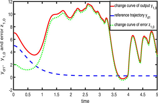
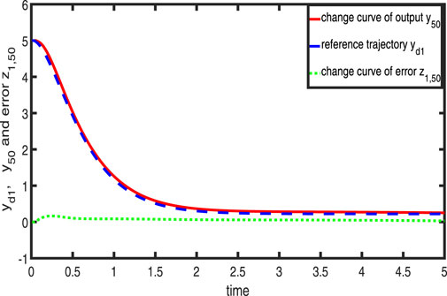
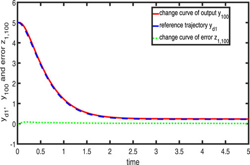
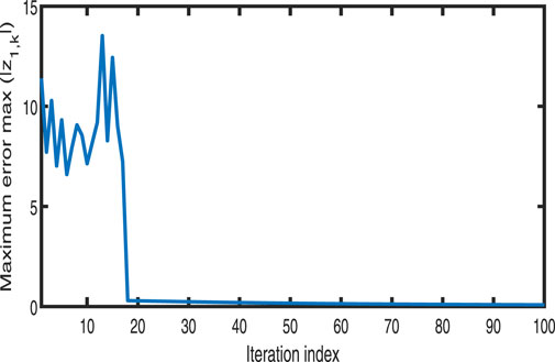
Figures 13 show the tracking performance of the system output and expected output without iteration and at 50th and 100th iterations, respectively. Figures 4, 5 show that as the number of iterations increases, the system error may converge to a small region near the zero point. Furthermore, observations shown in Figures 610 confirm that both control signals uk and αk and estimated parameters, Ŵ1,k, Ŵ2,k, M̂1,k, M̂2,k, N̂1,k,and N̂2,k, exhibit bounded behavior within the [0,5] range. The validity of the control strategy presented in this research is reaffirmed by the simulation results shown in Figures 1120 over the interval [0,T].

Figure 1
www.frontiersin.org

Figure 1. Variation in y0,yd1,z1,0 over time without iteration.

Figure 2
www.frontiersin.org

Figure 2. Variation in y50,yd1,z1,50 over time during the 50th iteration.

Figure 3
www.frontiersin.org

Figure 3. Variation in y100,yd1,z1,100 over time during the 100th iteration.

Figure 4
www.frontiersin.org

Figure 4. Variation in max(|z1,k|) according to the iteration index.

Figure 5
www.frontiersin.org

Figure 5. Variation in max(|z2,k|) according to the iteration index.

Figure 6
www.frontiersin.org

Figure 6. Variation in uk according to the iteration index.

Figure 7
www.frontiersin.org

Figure 7. Variation in αk according to the iteration index.

Figure 8
www.frontiersin.org

Figure 8. Variation in Ŵ1,k and Ŵ2,k according to the iteration index.

Figure 9
www.frontiersin.org

Figure 9. Variation in M̂1,k and M̂2,k according to the iteration index.

Figure 10
www.frontiersin.org

Figure 10. Variation in N̂1,k and N̂2,k according to the iteration index.

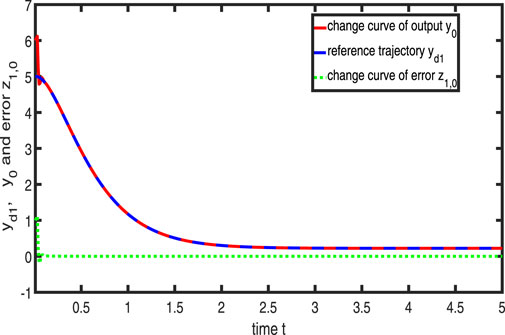
Figure 11
www.frontiersin.org

Figure 11. Variation in y0,yd1,z1,0 over time without iteration.

Figure 12
www.frontiersin.org

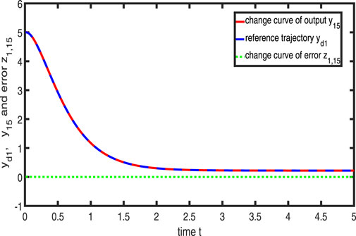
Figure 12. Variation in y15,yd1,z1,15 over time during the 15th iteration.

Figure 13
www.frontiersin.org

Figure 13. Variation in y30,yd1,z1,30 over time during the 30th iteration.

Figure 14
www.frontiersin.org

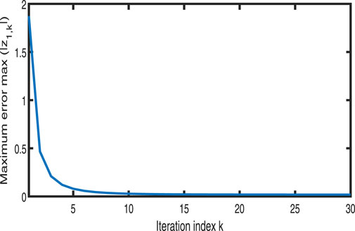
Figure 14. Variation in max(|z1,k|) according to the iteration index.

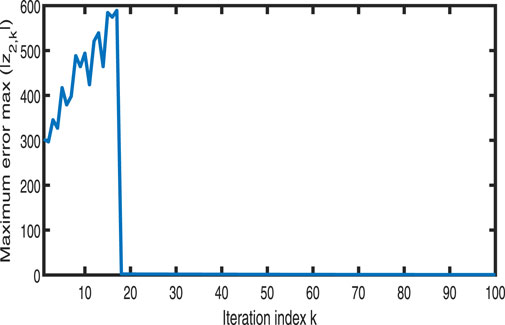
Figure 15
www.frontiersin.org

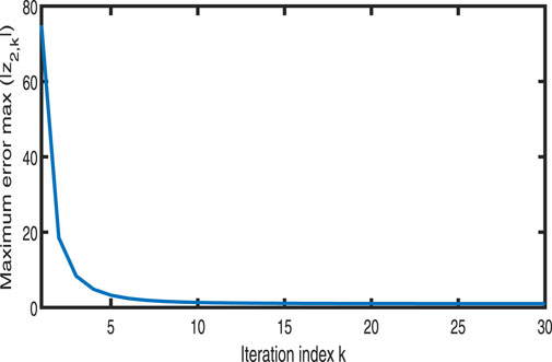
Figure 15. Variation in max(|z2,k|) according to the iteration index.

Figure 16
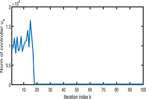
www.frontiersin.org

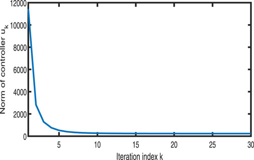
Figure 16. Variation in uk according to the iteration index.

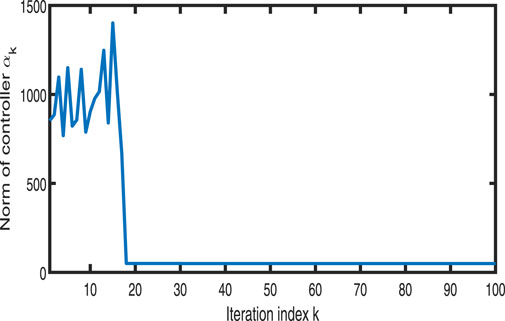
Figure 17
www.frontiersin.org

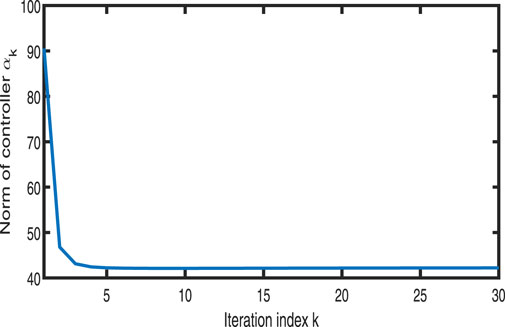
Figure 17. Variation in αk according to the iteration index.

Figure 18
www.frontiersin.org

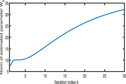
Figure 18. Variation of Ŵk according to the iteration index.

Figure 19
www.frontiersin.org

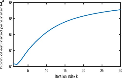
Figure 19. Variation in M̂k according to the iteration index.

Figure 20
www.frontiersin.org

Figure 20. Variation in N̂1,k and N̂2,k according to the iteration index.

4.2 Simulation of a single-joint robotic arm

In this section, we conducted simulation verification on a single degree-of-freedom robotic arm system to assess the performance of the proposed control method. The dynamic equation of a single degree-of-freedom robotic arm is

2θt2=10sinθ2θt+u,(88)

where θ is the angle between the robotic arm and the reference frame.u is the input of the DC motor.

2yd1t2=9yd16yd1t+2r,(89)

where yd1 is the output of the reference model. r is the reference input signal. According to Equations 88, 89, the state equation of the system is derived as

ẋ1,k=x2,kẋ2,k=10sinx1,k2x2,k+ukyk=x1,k,(90)

and its reference model is derived as

ẋd1=xd2ẋd2=9xd16xd2+2ryd1=xd1,(91)

where x1,k equals to θ can be defined as the angle between the robotic arm and the reference frame. x2,k is the time derivative of θ, i.e., θ̇. The primary control objective is to synchronize the output of systems (88) with the reference trajectory yd1 generated by system (89) over the interval [0,5] under the condition k.

In accordance with Theorem 1, the adaptive iterative learning controller is chosen as

α1,k=N̂1,k1Δkz1ϕ,k+ẏd1η1z1,kuk=z1ϕ,kc2z2,kŴ2,kTS2x̄2,k,M̂2,kTΦ2tN̂2,k1Δkz2ϕ,k+β̇1,k.(92)

The error compensation mechanism is

ζ̇1,k=β1,k+ζ2,kη1ζ1,kα1,kζ̇2,k=η2ζ2,kζ1,k,(93)

where β1,k=ξ(β1,kα1,k).

The parameter adaptive iterative learning laws are provided by (57).

Ŵ̇k=ΓfSx̄2,k,M̂kTΦtŜkM̂kTΦ2tz2ϕ,k,(94)
N̂̇i,k=ΓNi1Δkziϕ,k2,i=1,2,(95)
M̂̇k=ΓmΦtŴkTŜkz2ϕ,k,(96)

where c1=50, c2=150,Δk=a/k2, a=50000, Γ11=diag{1,1,1,1,1}, Γ21=10, Γ12=diag{1,1,1,1,1}, Γ22=1,andξ=10.

Figures 1113 show the tracking performance of the system output and expected output without iteration and at 15th and 30th iterations, respectively. Figures 14, 15 show that as the number of iterations increases, the system error may converge to a small region near the zero point. Furthermore, observations from Figures 1620 confirm that both control signals uk and αk and estimated parameters, Ŵk, M̂k, N̂1,k, and N̂2,k, exhibit bounded behavior within the [0,5] range. The validity of the control strategy presented in this research is reaffirmed by the simulation results shown in Figures 1120 over the interval [0,T].

5 Conclusion

This article presents a solution to the complete trajectory, following challenges within a finite time frame for a category of nonlinearly parameterized systems characterized by time-varying disturbed functions and initial state errors. A new FSE neural network is used to learn the time-varying, nonlinearly parameterized term. Based on this and Lyapunov theory, we proposed the new LPF-AILC method. A low-pass filter is used to solve the problem of parameter explosion after obtaining the derivative of the virtual controller. The unmatched uncertainties, nonlinear parameterization, and initial state errors are well considered. Two simulation examples have proven the feasibility of the control approach. This article does not mention time-delay issues, but they often exist in practical systems. Our future work should consider solving the complete tracking problem on a finite time interval for these complex systems with time delays. This is a more interesting issue. In addition, there are two deficiencies in the controller design process: the assumption of time-varying parameters being periodic and the jitter issues caused by the low-pass filter. These challenges will be carefully considered and addressed in our future work.

Data availability statement

The raw data supporting the conclusions of this article will be made available by the authors, without undue reservation.

Author contributions

CZ: conceptualization, funding acquisition, investigation, methodology, and writing–review and editing. LY: formal analysis, software, writing–original draft, and writing–review and editing. YG: investigation, validation, and writing–original draft. JY: funding acquisition, supervision, and writing–review and editing. FQ: funding acquisition, supervision, and writing–review and editing.

Funding

The authors declare that financial support was received for the research, authorship, and/or publication of this article. This work is supported by the National Natural Science Foundation (NNSF) of China (grants 62073259 and 61973094), the Natural Science Basis Research Plan in Shaanxi Province of China (2023-JC-QN-0752), the Science and Technology Plan Project of Xi’an City (No. 23GXFW0062), and the Shaanxi Provincial Key R& D Program General Project (No. 2024GX-YBXM-106).

Conflict of interest

The authors declare that the research was conducted in the absence of any commercial or financial relationships that could be construed as a potential conflict of interest.

Publisher’s note

All claims expressed in this article are solely those of the authors and do not necessarily represent those of their affiliated organizations, or those of the publisher, the editors, and the reviewers. Any product that may be evaluated in this article, or claim that may be made by its manufacturer, is not guaranteed or endorsed by the publisher.

References

1. Arimoto S, Kawamura S, Miyazaki F. Bettering operation of robots by learning. J Robot Syst (1984) 1(2):123–40. doi:10.1002/rob.4620010203

CrossRef Full Text | Google Scholar

2. Moore KL. Iterative learning control for Deterministic. London: Springer-Verlag (1993).

Google Scholar

3. Ahn HS, Chen YQ, Moore KL. Iterative learning control: brief survey and categorization. IEEE Trans Syst Man Cybernetics-C, Appl Rev (2007) 37(6):1099–121. doi:10.1109/tsmcc.2007.905759

CrossRef Full Text | Google Scholar

4. Xu J-X, Yan R, Chen Y-Q. “On initial conditions in iterative learning control,” in 2006 American Control Conference, Minneapolis, MN, United States (2006). doi:10.1109/ACC.2006.1655358

CrossRef Full Text | Google Scholar

5. Chen Y, Huang D, Xu C, Dong H. Iterative learning tracking control of high-speed trains with nonlinearly parameterized uncertainties and multiple time-varying delays. IEEE Trans Intell Transportation Syst (2022) 23(11):20476–88. doi:10.1109/tits.2022.3183608

CrossRef Full Text | Google Scholar

6. Zhang C, Yan L, Gao Y, Wang W, Li K, Wang D, et al. A new adaptive iterative learning control of finite-time hybrid function projective synchronization for unknown time-varying chaotic systems. Front Phys (2023) 11:1127884. doi:10.3389/fphy.2023.1127884

CrossRef Full Text | Google Scholar

7. Lu Y. Adaptive-Fuzzy control compensation design for direct adaptive fuzzy control. IEEE Trans Fuzzy Syst (2018) 26(6):3222–31. doi:10.1109/tfuzz.2018.2815552

CrossRef Full Text | Google Scholar

8. Yang Z, Wang S. Adaptive prescribed performance control for nonlinear robotic systems. J Franklin Inst (2023) 360(2):1378–94. doi:10.1016/j.jfranklin.2022.10.044

CrossRef Full Text | Google Scholar

9. Kong X, Yu F, Yao W, Cai S, Zhang J, Lin H. Memristor-induced hyperchaos, multiscroll and extreme multistability in fractional-order HNN: image encryption and FPGA implementation. Neural Networks (2024) 171:85–103. doi:10.1016/j.neunet.2023.12.008

PubMed Abstract | CrossRef Full Text | Google Scholar

10. Yu F, Kong X, Yao W, Zhang J, Cai S, Lin H, et al. Dynamics analysis, synchronization and FPGA implementation of multiscroll Hopfield neural networks with non-polynomial memristor. Chaos, Solitons & Fractals (2024) 179:114440. Article ID 114440. doi:10.1016/j.chaos.2023.114440

CrossRef Full Text | Google Scholar

11. Hu X, Xu B, Hu C. Robust adaptive fuzzy control for HFV with parameter uncertainty and unmodeled dynamics. IEEE Trans Ind Electronics (2018) 65(11):8851–60. doi:10.1109/tie.2018.2815951

CrossRef Full Text | Google Scholar

12. Liu Z, Shi J, Zhao X, Zhao Z, Li H -X. Adaptive fuzzy event-triggered control of aerial refueling hose system with actuator failures. IEEE Trans Fuzzy Syst (2022) 30(8):2981–92. doi:10.1109/tfuzz.2021.3098733

CrossRef Full Text | Google Scholar

13. Hu X, Li Y -X, Tong S, Hou Z. Event-triggered adaptive fuzzy asymptotic tracking control of nonlinear pure-feedback systems with prescribed performance. IEEE Trans Cybernetics (2023) 53(4):2380–90. doi:10.1109/tcyb.2021.3118835

CrossRef Full Text | Google Scholar

14. Zhang C, Tian X, Yan L. Adaptive iterative learning control method for finite-time tracking of an aircraft track angle system based on a neural network. Front Phys (2022) 10:1048942. doi:10.3389/fphy.2022.1048942

CrossRef Full Text | Google Scholar

15. Pang N, Wang X, Wang Z. Event-triggered adaptive control of nonlinear systems with dynamic uncertainties: the switching threshold case. IEEE Trans Circuits Syst Express Briefs (2022) 69(8):3540–4. doi:10.1109/tcsii.2022.3164572

CrossRef Full Text | Google Scholar

16. Liu X, Xu B, Cheng Y, Wang H, Chen W. Adaptive control of uncertain nonlinear systems via event-triggered communication and NN learning. IEEE Trans Cybernetics (2023) 53(4):2391–401. doi:10.1109/tcyb.2021.3119780

CrossRef Full Text | Google Scholar

17. Yang X, Zheng X. Gradient descent algorithm-based adaptive NN control design for an induction motor. IEEE Trans Syst Man, Cybernetics: Syst (2021) 51(2):1027–34. doi:10.1109/tsmc.2019.2894661

CrossRef Full Text | Google Scholar

18. Li K, Li Y. Adaptive neural network finite-time dynamic surface control for nonlinear systems. IEEE Trans Neural Networks Learn Syst (2021) 32(12):5688–97. doi:10.1109/tnnls.2020.3027335

CrossRef Full Text | Google Scholar

19. Lin H, Deng X, Yu F, Sun Y. Grid multi-butterfly memristive neural network with three memristive systems: modeling, dynamic analysis, and application in police IoT. IEEE Internet Things J (2024) 1. doi:10.1109/jiot.2024.3409373

CrossRef Full Text | Google Scholar

20. Li J, Wang C, Deng Q. Symmetric multi-double-scroll attractors in Hopfield neural network under pulse controlled memristor. Nonlinear Dyn (2024) 112:14463–77. doi:10.1007/s11071-024-09791-6

CrossRef Full Text | Google Scholar

21. Chien CJ. A combined adaptive law for fuzzy iterative learning control of nonlinear systems with varying control tasks. IEEE Trans Fuzzy Syst (2008) 16(1):40–51. doi:10.1109/tfuzz.2007.902021

CrossRef Full Text | Google Scholar

22. Xu JX, Yan R. Adaptive learning control for finite interval tracking based on constructive function approximation and wavelet. IEEE Trans Neural Networks (2011) 22(6):893–905. doi:10.1109/tnn.2011.2132143

PubMed Abstract | CrossRef Full Text | Google Scholar

23. Taybi A, Chien CJ. A unified adaptive iterative learning control framework for uncertain nonlinear systems. IEEE Trans Automatic Control (2007) 52(10):1907–13. doi:10.1109/TAC.2007.906215

CrossRef Full Text | Google Scholar

24. Ji H, Hou Z, Zhang R. Adaptive iterative learning control for high-speed trains with unknown speed delays and input saturations. IEEE Trans Automation Sci Eng (2016) 13(1):260–73. doi:10.1109/tase.2014.2371816

CrossRef Full Text | Google Scholar

25. Li JM, Wang YL, Li XM. Adaptive iterative learning control for nonlinear parameterized-systems with unknown time-varying delays. Control Theor Appl (2011) 28(6):861–8. doi:10.7641/j.issn.1000-8152.2011.6.ccta091224

CrossRef Full Text | Google Scholar

26. Zhang C-L, Li J-M. Adaptive iterative learning control for nonlinear time-delay systems with periodic disturbances using FSE-neural network. Int J Automation Comput (2011) 8(4):403–10. doi:10.1007/s11633-011-0597-x

CrossRef Full Text | Google Scholar

27. Park BH, Kuc TY, Lee JS. Adaptive learning of uncertain robotic systems. Int J Control (1996) 65(5):725–744. doi:10.1080/00207179608921719

CrossRef Full Text | Google Scholar

28. Choi JY, Lee JS. Adaptive iterative learning control of uncertain robotic systems. Proc Inst Elect Eng D (2000) 147(2):217–23. doi:10.1049/ip-cta:20000138

CrossRef Full Text | Google Scholar

29. Liu G, Hou Z. Adaptive iterative learning control for subway trains using multiple-point-mass dynamic model under speed constraint. IEEE Trans Intell Transportation Syst (2021) 22(3):1388–400. doi:10.1109/tits.2020.2970000

CrossRef Full Text | Google Scholar

30. Ji H, Hou Z, Zhang R. Adaptive iterative learning control for high-speed trains with unknown speed delays and input saturations. IEEE Trans Automation Sci Eng (2016) 13(1):260–73. doi:10.1109/tase.2014.2371816

CrossRef Full Text | Google Scholar

31. Geng Y, Ruan X, Xu J. Adaptive iterative learning control of switched nonlinear discrete-time systems with unmodeled dynamics. IEEE Access (2019) 7:118370–80. doi:10.1109/access.2019.2936763

CrossRef Full Text | Google Scholar

32. Heinzinger G, Fenwick D, Paden B, Miyazaki F. Stability of learning control with disturbances and uncertain initial conditions. IEEE Trans Automat Contr (1992) 37:110–4. doi:10.1109/9.109644

CrossRef Full Text | Google Scholar

33. Chien CJ, Liu JS. AP-type iterative learning controller for robust output tracking of nonlinear time-varying systems. Int J Control (1996) 64(2):319–34. doi:10.1080/00207179608921630

CrossRef Full Text | Google Scholar

34. Park KH, Bien Z, Hwang DH. A study on the robustness of a PID-type iterative learning controller against initial state error. Int J Syst Sci (1999) 30(1):49–59. doi:10.1080/002077299292669

CrossRef Full Text | Google Scholar

35. Sun M, Wang D. Iterative learning control with initial rectifying action. Automatica (2002) 38:1177–82. doi:10.1016/s0005-1098(02)00003-1

CrossRef Full Text | Google Scholar

36. Chien CJ, Hsu CT, Yao CY. Fuzzy system based adaptive iterative learning control for nonlinear plants with initial state errors. IEEE Trans Fuzzy Syst (2004) 12(5):724–32. doi:10.1109/tfuzz.2004.834806

CrossRef Full Text | Google Scholar

37. Wu XJ, Wu XL, Ran Zhen XY, Luo XJ, Zhu QM. Adaptive control for time-delay non-linear systems with non-symmetric input non-linearity. Int J Model Identification Control (2011) 13(3):152–60. doi:10.1504/ijmic.2011.041302

CrossRef Full Text | Google Scholar

38. Luo XY, Wu XJ, Guan XP. Adaptive backstepping fault-tolerant controlfor unmatched non-linear systems against actuator dead-zone. IET Control Theor Appl. (2010) 4(5):879–88. doi:10.1049/iet-cta.2009.0086

CrossRef Full Text | Google Scholar

39. Wu X, Wu X, Luo X, Zhu Q, Guan X. Neural network-based adaptive tracking control for nonlinearly parameterized systems with unknown input nonlinearities. Neurocomputing (2012) 82:127–42. doi:10.1016/j.neucom.2011.10.019

CrossRef Full Text | Google Scholar

40. Chen WS. Adaptive backstepping dynamic surface control for systems with periodic disturbances using neural networks. IET Control Theor Appl (2009) 3(10):1383–94. doi:10.1049/iet-cta.2008.0322

CrossRef Full Text | Google Scholar

41. Zhu S, Ming-Xuan SUN, Xiong-Xiong HE. Iterative learning control of strict-feedback nonlinear time-varying systems. ACTA AUTOMATICA SINICA (2010) 36(3):454–8. doi:10.3724/SP.J.1004.2010.00454

CrossRef Full Text | Google Scholar

42. Yu H, Li Y. Adaptive obstacle avoidance control based on first-order low-pass filter for cleaning robots. Marseille, France: OCEANS 2019 - Marseille (2019). p. 1–6.

Google Scholar

43. Zhang C, Tian X, Gao Y, Qian F. Command filter AILC for finite time accurate tracking of aircraft track angle system based on fuzzy logic. Adv Math Phys (2023) 2023:11. Article ID 4744873. doi:10.1155/2023/4744873

CrossRef Full Text | Google Scholar

44. Huang J -T, Pham T -P. Differentiation-free multiswitching neuroadaptive control of strict-feedback systems. IEEE Trans Neural Networks Learn Syst (2017) 29(4):1095–107. doi:10.1109/tnnls.2017.2651903

CrossRef Full Text | Google Scholar

Keywords: adaptive iterative learning control, time-varying non-parameterized nonlinear systems, backstepping method, Fourier series expansion-radial basis function neural network, initial state errors, low-pass filter

Citation: Zhang C, Yan L, Gao Y, Yao J and Qian F (2024) FSE-RBFNN-based LPF-AILC of finite time complete tracking for a class of time-varying NPNL systems with initial state errors. Front. Phys. 12:1442486. doi: 10.3389/fphy.2024.1442486

Received: 02 June 2024; Accepted: 02 August 2024;
Published: 21 August 2024.

Edited by:

Fei Yu, Changsha University of Science and Technology, China

Reviewed by:

Jinping Jia, Tianshui Normal University, China
Yichao Yan, University of Electronic Science and Technology of China, China
Njitacke Tabekoueng Zeric, University of Buea, Cameroon

Copyright © 2024 Zhang, Yan, Gao, Yao and Qian. This is an open-access article distributed under the terms of the Creative Commons Attribution License (CC BY). The use, distribution or reproduction in other forums is permitted, provided the original author(s) and the copyright owner(s) are credited and that the original publication in this journal is cited, in accordance with accepted academic practice. No use, distribution or reproduction is permitted which does not comply with these terms.

*Correspondence: Junliang Yao, yaojunliang@xaut.edu.cn

ORCID: Lei Yan, orcid.org/0000-0001-5894-7588; Yangjie Gao, orcid.org/0009-0009-9651-5757; Junliang Yao, orcid.org/0000-0001-6041-9813; Fucai Qian, orcid.org/0000-0001-8461-1420

Disclaimer: All claims expressed in this article are solely those of the authors and do not necessarily represent those of their affiliated organizations, or those of the publisher, the editors and the reviewers. Any product that may be evaluated in this article or claim that may be made by its manufacturer is not guaranteed or endorsed by the publisher.