A comparative analytical investigation for some linear and nonlinear time-fractional partial differential equations in the framework of the Aboodh transformation

This article discusses two simple, complication-free, and effective methods for solving fractional-order linear and nonlinear partial differential equations analytically: the Aboodh residual power series method (ARPSM) and the Aboodh transform iteration method (ATIM). The Caputo operator is utilized to define fractional order derivatives. In these methods, the analytical approximations are derived in series form. We calculate the first terms of the series and then estimate the absolute error resulting from leaving out the remaining terms to ensure the accuracy of the derived approximations and determine the accuracy and efficiency of the suggested methods. The derived approximations are discussed numerically using some values for the relevant parameters to the subject of the study. Useful examples are thought to illustrate the practical application of current approaches. We also examine the fractional order results that converge to the integer order solutions to ensure the accuracy of the derived approximations. Many researchers, particularly those in plasma physics, are anticipated to gain from modeling evolution equations describing nonlinear events in plasma systems.

1 Introduction

Noninteger calculus is a prominent branch of mathematics that employs fractional order operators to mimic and clarify physical processes. Another facet of this topic is the application of noninteger order derivatives to both integration and differentiation difficulties. For zero-order the ordinary derivative is recovered. A fractional derivative has a noninteger order and meets specific conditions [1]. A few of the benefits of fractional derivatives include the memory effect and preserved demonstrative physical qualities. Using these operators, more recent and accurate research has been discovered. Thus, the theory and practice of fractional calculus are seeing a surge in popularity. The memory effect allows fractional order models to absorb all prior information, which improves their ability to anticipate and evaluate dynamical models. The efficient characteristics of fractional order calculus make it applicable to numerous fields, including biology and physics [2–6] economics and finance [7, 8], mechanical modeling and mathematical modeling, and [9–11] science and engineering. The singularity of the kernel in Caputo and Riemann derivatives presents a challenge for the authors. Given that the kernel is employed to elucidate the memory impact of the physical system, it is evident that this constraint prevents both derivatives from precisely interpreting the memory’s complete effect [12–14]. In an endeavor to develop a novel fractional operator featuring an exponential kernel, Caputo and Fabrizio (CF) [15] proposed one in the mid-nineties. The nonsingular kernel of this derivative yields more rational results than the classical approach. A selection of CF operator applications is detailed in [16–18].

There are two categories of partial differential equations: linear and nonlinear. Solving a fractional-order partial differential equation accurately is a difficult task. However, developing numerical and exact solutions to these equations is crucial in applied mathematics and theoretical physics [19–21]. Consequently, innovative methods have been developed for analytical solutions that closely approximate the exact solutions [22, 23]. Differential equations were often solved using integral transforms. Integral transformations are helpful in solving initial value problems (IVPs) and boundary value problems (BVPs) in differential and integral equations. A wide range of authors investigated the effects of diverse types of integral transforms implemented on various categories of differential equations. The most frequently employed integral transform is the Laplace transform [24]. Watugala [25] introduced the Sumudu transform in 1998 as a powerful technique for solving differential equations and addressing engineering problems. T. Elzaki and S. Elzaki [26] introduced the “Elzaki Transform” as a new integral transform in 2011, which is extensively used in solving partial differential equations. Aboodh introduced the “Aboodh Transform” in 2013 and applied it to address partial differential equations (27). Numerous transformations are present in the literature.

In 2013, Omar Abu Arqub developed the RPSM [28]. The RPSM is a semi-analytical approach that combines Taylor’s series with the residual error function. Convergence series for nonlinear and linear DEs are both solved using it. In 2013, RPSM was first used to resolve fuzzy differential equations. To quickly get power series solutions for common DEs, Arqub et al. [29] created a novel RPSM method. Arqub et al. [30] developed a unique and appealing RPSM technique for fractional DEs issues. El-Ajou et al. [31] proposed a special iterative technique using RPSM to estimate fractional KdV-burger equations. Xu et al. [32] introduced a novel approach for solving Boussinesq DEs using fractional power series. Zhang et al. devised a robust numerical approach [33]. For further information on RPSM, see [34–36].

Differential equations have been crucial in several aspects of applied mathematics and theoretical physics for an extended period, and their importance has increased with the advent of computers [37, 38]. Examining and analyzing differential equations used in applications reveal numerous intricate mathematical challenges, resulting in various methods for solving them. Various integral transforms, such as Laplace, Fourier, Mellin, Hankel, and Sumudu, were commonly used for solving differential equations. Khalid Aboodh introduced a new integral transform called the Aboodh transform and applied it to solve both ordinary and partial differential equations (39)–(41).

The Aboodh residual power series method (ARPSM) [42, 43] and the Aboodh transform iteration method (ATIM) [39–41] are regarded as the most straightforward methods to solve fractional differential equations. These approaches give numeric results for partial differential equations that do not need discretization or linearization and make the symbol elements of analytic solutions more visible and accessible. The fundamental goal of this research is to contrast and evaluate the efficacy of ARPSM and ATIM in solving linear and nonlinear PDE problems. It is worth noting that many linear and nonlinear fractional differential equations have been solved using these two approaches.

2 Elementary concepts

Definition 2.1. [44] The function ϕ(α, β) is assumed to be piecewise continuous and of exponential order.

For ϕ(α, β) and τ ≥ 0 Aboodh transform (AT) is given as:

$A\left[\varphi \left(\alpha ,\beta \right)\right]=\mathrm{\Psi }\left(\alpha ,\xi \right)=\frac{1}{\xi }{\int }_0^{\infty }\varphi \left(\alpha ,\beta \right)e^{-\beta \xi }d\beta ,r_1\le \xi \le r_2.$

The Aboodh inverse transform (AIT) is described as:

$A^{-1}\left[\mathrm{\Psi }\left(\alpha ,\xi \right)\right]=\varphi \left(\alpha ,\beta \right)=\frac{1}{2\pi i}{\int }_{u-i\infty }^{u+i\infty }\mathrm{\Psi }\left(\alpha ,\beta \right)\xi e^{\beta \xi }d\beta$

Where $\alpha =({\alpha }_1,{\alpha }_2,\dots ,{\alpha }_p)\in \mathbb{R}$ and $p\in \mathbb{N}$

Lemma 2.1. [45, 46] Define two functions ϕ₁(α, ϕ₂β) that are piecewise continuous on [0, ∞[ and of exponential order. Suppose that A[ϕ₁(α, β)] = Ψ₁(α, β), A[ϕ₂(α, β)] = Ψ₂(α, β) and λ₁, λ₂ are constants. Consequently, the following characteristics hold:

1. A [λ₁ϕ₁ (α, β) + λ₂ϕ₂ (α, β)] = λ₁Ψ₁ (α, ξ) + λ₂Ψ₂ (α, β),

2. A⁻¹ [λ₁Ψ₁ (α, β) + λ₂Ψ₂ (α, β)] = λ₁ϕ₁ (α, ξ) + λ₂ϕ₂ (α, β),

3. $A[J_{\beta }^p\varphi (\alpha ,\beta )]=\frac{\mathrm{\Psi }(\alpha ,\xi )}{{\xi }^p}$,

4. $A[D_{\beta }^p\varphi (\alpha ,\beta )]={\xi }^p\mathrm{\Psi }(\alpha ,\xi )-{\displaystyle {\sum }_{K=0}^{r-1}}\frac{{\varphi }^K(\alpha ,0)}{{\xi }^{K-p+2}},r-1<p\le r,r\in \mathbb{N}$.

Definition 2.2. [47] The fractional derivative of the function ϕ(α, β) is defined in terms of order p according to the Caputo.

$D_{\beta }^p\varphi \left(\alpha ,\beta \right)=J_{\beta }^{m-p}{\varphi }^{\left(m\right)}\left(\alpha ,\beta \right),r\ge 0,m-1<p\le m,$

where $\alpha =({\alpha }_1,{\alpha }_2,\dots ,{\alpha }_p)\in {\mathbb{R}}^p$ and $m,p\in R,J_{\beta }^{m-p}$ is the R-L integral of ϕ(α, β).

Definition 2.3. [48] The following is the form of the power series representation.

${\displaystyle \sum _{r=0}^{\infty }}{\hslash }_r\left(\alpha \right){\left(\beta -{\beta }_0\right)}^{rp}={\hslash }_0{\left(\beta -{\beta }_0\right)}^0+{\hslash }_1{\left(\beta -{\beta }_0\right)}^p+{\hslash }_2{\left(\beta -{\beta }_0\right)}^{2p}+\cdots ,$

where $\alpha =({\alpha }_1,{\alpha }_2,\dots ,{\alpha }_p)\in {\mathbb{R}}^p$ and $p\in \mathbb{N}$. This series is called multiple fractional power series (MFPS) about β₀, where the series coefficients are ℏ_r(α)′s and β is variable.

Lemma 2.2. Let us suppose that the exponential order function is ϕ(α, β). In such case, the AT is defined as A[ϕ(α, β)] = Ψ(α, ξ). Hence,

$A\left[D_{\beta }^{rp}\varphi \left(\alpha ,\beta \right)\right]={\xi }^{rp}\mathrm{\Psi }\left(\alpha ,\xi \right)-{\displaystyle \sum _{j=0}^{r-1}}{\xi }^{p\left(r-j\right)-2}{D}_{\beta }^{jp}\varphi \left(\alpha ,0\right),0<p\le 1,(1)$

where $\alpha =({\alpha }_1,{\alpha }_2,\dots ,{\alpha }_p)\in {\mathbb{R}}^p$ and $p\in \mathbb{N}$ and $D_{\beta }^{rp}=D_{\beta }^p.D_{\beta }^p.\cdots .D_{\beta }^p(r-times)$

Proof. Using induction, we can prove Eq. 2. Choosing r = 1 in Eq. 2 leads to the following results:

$A\left[D_{\beta }^{2p}\varphi \left(\alpha ,\beta \right)\right]={\xi }^{2p}\mathrm{\Psi }\left(\alpha ,\xi \right)-{\xi }^{2p-2}\varphi \left(\alpha ,0\right)-{\xi }^{p-2}{D}_{\beta }^p\varphi \left(\alpha ,0\right)$

Lemma 2.1, part (4), states that Eq. 2 is true for r = 1. By substituting r = 2 into Eq. 2, we have

$A\left[D_r^{2p}\varphi \left(\alpha ,\beta \right)\right]={\xi }^{2p}\mathrm{\Psi }\left(\alpha ,\xi \right)-{\xi }^{2p-2}\varphi \left(\alpha ,0\right)-{\xi }^{p-2}{D}_{\beta }^p\varphi \left(\alpha ,0\right).(2)$

Based on Eq. 2 L.H.S, we may deduce

$L.H.S=A\left[D_{\beta }^{2p}\varphi \left(\alpha ,\beta \right)\right].(3)$

One possible way to express Eq. 3 is as:

$L.H.S=A\left[D_{\beta }^p\varphi \left(\alpha ,\beta \right)\right].(4)$

Suppose

$z\left(\alpha ,\beta \right)=D_{\beta }^p\varphi \left(\alpha ,\beta \right).(5)$

Equation 4 therefore becomes as

$L.H.S=A\left[D_{\beta }^{p}z\left(\alpha ,\beta \right)\right].(6)$

Due to the utilization of the derivative of Caputo, Eq. 6 modified as.

$L.H.S=A\left[J^{1-p}{z}^{\prime }\left(\alpha ,\beta \right)\right].(7)$

Equation 7 contains the R-L integral for AT, which enables the following to be obtained:

$L.H.S=\frac{A\left[z^{\prime }\left(\alpha ,\beta \right)\right]}{{\xi }^{1-p}}.(8)$

Using the differential property of the AT, Eq. 8 is converted to the following form:

$L.H.S={\xi }^{p}Z\left(\alpha ,\xi \right)-\frac{z\left(\alpha ,0\right)}{{\xi }^{2-p}},(9)$

Eq. 5 gives us the following:

$Z\left(\alpha ,\xi \right)={\xi }^p\mathrm{\Psi }\left(\alpha ,\xi \right)-\frac{\varphi \left(\alpha ,0\right)}{{\xi }^{2-p}},$

where A [z (α, β)] = Z (α, ξ). Therefore, Eq. 9 is converted to

$L.H.S={\xi }^{2p}\mathrm{\Psi }\left(\alpha ,\xi \right)-\frac{\varphi \left(\alpha ,0\right)}{{\xi }^{2-2p}}-\frac{D_{\beta }^p\varphi \left(\alpha ,0\right)}{{\xi }^{2-p}},(10)$

when r = K. Eq. 10 is compatible with Eq. 2. Suppose that for r = K, Eq. 2 holds true. As a result, we may substitute r = K into Eq. 2:

$A\left[D_{\beta }^{Kp}\varphi \left(\alpha ,\beta \right)\right]={\xi }^{Kp}\mathrm{\Psi }\left(\alpha ,\xi \right)-{\displaystyle \sum _{j=0}^{K-1}}{\xi }^{p\left(K-j\right)-2}{D}_{\beta }^{jp}{D}_{\beta }^{jp}\varphi \left(\alpha ,0\right),0<p\le 1.(11)$

The next step is to illustrate Eq. 2 for the value of r = K + 1. Using Eq. 2, we can write

$A\left[D_{\beta }^{\left(K+1\right)p}\varphi \left(\alpha ,\beta \right)\right]={\xi }^{\left(K+1\right)p}\mathrm{\Psi }\left(\alpha ,\xi \right)-{\displaystyle \sum _{j=0}^K}{\xi }^{p\left(\left(K+1\right)-j\right)-2}{D}_{\beta }^{jp}\varphi \left(\alpha ,0\right).(12)$

When the LHS of Eq. 12 is taken into consideration, we get

$L.H.S=A\left[D_{\beta }^{Kp}\left(D_{\beta }^{Kp}\right)\right].(13)$

Let

$D_{\beta }^{Kp}=g\left(\alpha ,\beta \right).$

By Eq. 13, we get

$L.H.S=A\left[D_{\beta }^{p}g\left(\alpha ,\beta \right)\right].(14)$

Equation 14 is transformed into the following using the R-L integral and derivative of Caputo.

$L.H.S={\xi }^{p}A\left[D_{\beta }^{Kp}\varphi \left(\alpha ,\beta \right)\right]-\frac{g\left(\alpha ,0\right)}{{\xi }^{2-p}}.(15)$

By ulatizing Eq. 11 and Eq. 15 becomes

$L.H.S={\xi }^{rp}\mathrm{\Psi }\left(\alpha ,\xi \right)-{\displaystyle \sum _{j=0}^{r-1}}{\xi }^{p\left(r-j\right)-2}{D}_{\beta }^{jp}\varphi \left(\alpha ,0\right),(16)$

further, the following result is derived from Eq. 16.

$L.H.S=A\left[D_{\beta }^{rp}\varphi \left(\alpha ,0\right)\right].$

Consequently, for r = K + 1, Eq. 2 is true. In light of this, we showed that Eq. 2 holds for every positive integer by applying the mathematical induction method.

A novel version of multiple fractional Taylor’s series (MFTS) is shown in the following lemma. This formula will be helpful for the ARPSM, which will be discussed further below.

Lemma 2.3. Let’s assume ϕ(α, β) be the exponential order function. The AT of ϕ(α, β), which is represented by the expression A[ϕ(α, β)] = Ψ(α, ξ), is characterized by a MFTS notation as:

$\mathrm{\Psi }\left(\alpha ,\xi \right)={\displaystyle \sum _{r=0}^{\infty }}\frac{{\hslash }_r\left(\alpha \right)}{{\xi }^{rp+2}},\xi >0,(17)$

where, $\alpha =(s_1,{\alpha }_2,\dots ,{\alpha }_p)\in {\mathbb{R}}^p,p\in \mathbb{N}$.

Proof. Let us analyze Taylor’s series expressed in fractional order as

$\varphi \left(\alpha ,\beta \right)={\hslash }_0\left(\alpha \right)+{\hslash }_1\left(\alpha \right)\frac{{\beta }^p}{\mathrm{\Gamma }\left[p+1\right]}++{\hslash }_2\left(\alpha \right)\frac{{\beta }^{2p}}{\mathrm{\Gamma }\left[2p+1\right]}+\cdots .(18)$

Applying the AT to Eq. 18 yields the subsequent equality:

$A\left[\varphi \left(\alpha ,\beta \right)\right]=A\left[{\hslash }_0\left(\alpha \right)\right]+A\left[{\hslash }_1\left(\alpha \right)\frac{{\beta }^p}{\mathrm{\Gamma }\left[p+1\right]}\right]+A\left[{\hslash }_1\left(\alpha \right)\frac{{\beta }^{2p}}{\mathrm{\Gamma }\left[2p+1\right]}\right]+\cdots$

This is achieved by employing the properties of the AT.

$A\left[\varphi \left(\alpha ,\beta \right)\right]={\hslash }_0\left(\alpha \right)\frac{1}{{\xi }^2}+{\hslash }_1\left(\alpha \right)\frac{\mathrm{\Gamma }\left[p+1\right]}{\mathrm{\Gamma }\left[p+1\right]}\frac{1}{{\xi }^{p+2}}+{\hslash }_2\left(\alpha \right)\frac{\mathrm{\Gamma }\left[2p+1\right]}{\mathrm{\Gamma }\left[2p+1\right]}\frac{1}{{\xi }^{2p+2}}\cdots$

As a result, 17, which is a novel variant of Taylor’s series in the AT, is acquired.

Lemma 2.4. Let A[ϕ(α, β)] = Ψ(α, ξ) be the MFPS stated in the new form of Taylor’s series 17. Then we have

${\hslash }_0\left(\alpha \right)=\underset{\xi \to \infty }{\lim }{\xi }^2\mathrm{\Psi }\left(\alpha ,\xi \right)=\varphi \left(\alpha ,0\right).(19)$

Proof. From the Taylor’s series new form, the preceding is derived:

${\hslash }_0\left(\alpha \right)={\xi }^2\mathrm{\Psi }\left(\alpha ,\xi \right)-\frac{{\hslash }_1\left(\alpha \right)}{{\xi }^p}-\frac{{\hslash }_2\left(\alpha \right)}{{\xi }^{2p}}-\cdots (20)$

After applying lim_ξ→∞ to Eq. 19 and doing a short computation, we get the necessary result, which is shown by 20.

Theorem 2.5. Let the MFPS notation of the function A[ϕ(α, β)] = Ψ(α, ξ) is provided by

$\mathrm{\Psi }\left(\alpha ,\xi \right)={\displaystyle \sum _0^{\infty }}\frac{{\hslash }_r\left(\alpha \right)}{{\xi }^{rp+2}},\xi >0,$

where $\alpha =({\alpha }_1,{\alpha }_2,\dots ,{\alpha }_p)\in {\mathbb{R}}^p$ and $p\in \mathbb{N}$. Then we have

${\hslash }_r\left(\alpha \right)=D_r^{rp}\varphi \left(\alpha ,0\right),$

where, $D_{\beta }^{rp}=D_{\beta }^p.D_{\beta }^p.\cdots .D_{\beta }^p(r-times)$.

Proof. We have the Taylor’s series in its new form

${\hslash }_1\left(\alpha \right)={\xi }^{p+2}\mathrm{\Psi }\left(\alpha ,\xi \right)-{\xi }^p{\hslash }_0\left(\alpha \right)-\frac{{\hslash }_2\left(\alpha \right)}{{\xi }^p}-\frac{{\hslash }_3\left(\alpha \right)}{{\xi }^{2p}}-\cdots (21)$

Using Eq. 21 and lim_ξ→∞, we get

${\hslash }_1\left(\alpha \right)=\underset{\xi \to \infty }{\lim }\left({\xi }^{p+2}\mathrm{\Psi }\left(\alpha ,\xi \right)-{\xi }^p{\hslash }_0\left(\alpha \right)\right)-\underset{\xi \to \infty }{\lim }\frac{{\hslash }_2\left(\alpha \right)}{{\xi }^p}-\underset{\xi \to \infty }{\lim }\frac{{\hslash }_3\left(\alpha \right)}{{\xi }^{2p}}-\cdots$

Taking the linit, we arrive to the following equality:

${\hslash }_1\left(\alpha \right)=\underset{\xi \to \infty }{\lim }\left({\xi }^{p+2}\mathrm{\Psi }\left(\alpha ,\xi \right)-{\xi }^p{\hslash }_0\left(\alpha \right)\right).(22)$

The application of Lemma 2.2 to Eq. 22 results in the following:

${\hslash }_1\left(\alpha \right)=\underset{\xi \to \infty }{\lim }\left({\xi }^{2}A\left[D_{\beta }^p\varphi \left(\alpha ,\beta \right)\right]\left(\xi \right)\right).(23)$

Moreover, by using Lemma 2.3 to Eq. 23, it is transformed into

${\hslash }_1\left(\alpha \right)=D_{\beta }^p\varphi \left(\alpha ,0\right).$

Once more, by taking into account the new form of Taylor’s series and taking limit ξ → ∞, we conclude that

${\hslash }_2\left(\alpha \right)={\xi }^{2p+2}\mathrm{\Psi }\left(\alpha ,\xi \right)-{\xi }^{2p}{\hslash }_0\left(\alpha \right)-{\xi }^p{\hslash }_1\left(\alpha \right)-\frac{{\hslash }_3\left(\alpha \right)}{{\xi }^p}-\cdots$

As a result of Lemma 2.3, we get

${\hslash }_2\left(\alpha \right)=\underset{\xi \to \infty }{\lim }{\xi }^2\left({\xi }^{2p}\mathrm{\Psi }\left(\alpha ,\xi \right)-{\xi }^{2p-2}{\hslash }_0\left(\alpha \right)-{\xi }^{p-2}{\hslash }_1\left(\alpha \right)\right).(24)$

Using Lemmas 2.2 and 2.4, Eq. 24 becomes

${\hslash }_2\left(\alpha \right)=D_{\beta }^{2p}\varphi \left(\alpha ,0\right).$

Applying the same process to the new Taylor’s series yields the following results:

${\hslash }_3\left(\alpha \right)=\underset{\xi \to \infty }{\lim }{\xi }^2\left(A\left[D_{\beta }^{2p}\varphi \left(\alpha ,p\right)\right]\left(\xi \right)\right).$

Following the use of Lemma 2.4, the final equation is found.

${\hslash }_3\left(\alpha \right)=D_{\beta }^{3p}\varphi \left(\alpha ,0\right).$

In general

${\hslash }_r\left(\alpha \right)=D_{\beta }^{rp}\varphi \left(\alpha ,0\right).$

Thus, the proof concludes.

The subsequent theorem details and establishes the conditions that govern the convergence of the new form of Taylor’s series.

Theorem 2.6. The expression A[ϕ(α, β)] = Ψ(α, ξ) represents the new form of the formula for multiple fractional Taylor’s, which is presented in Lemma 2.3. If $|{\xi }^{a}A[D_{\beta }^{(K+1)p}\varphi (\alpha ,\beta )]|\le T$, on 0 < ξ ≤ s with 0 < p ≤ 1, then the following inequality is satisfied by the residual R_K(α, ξ) of the new version of MFTS:

$|R_K\left(\alpha ,\xi \right)|\le \frac{T}{{\xi }^{\left(K=1\right)p+2}},0<\xi \le s.$

Proof. Let $A[D_{\beta }^{rp}\varphi (\alpha ,\beta )](\xi )$ for r = 0, 1, 2, … , K + 1, is defined on 0 < ξ ≤ s. Assume, as given, that $|{\xi }^{2}A[D_{{\beta }^{K+1}}\varphi (\alpha ,tau)]|\le T,on0<\xi \le s$. Determine the following relationship based on the revised version of Taylor’s series:

$R_K\left(\alpha ,\xi \right)=\mathrm{\Psi }\left(\alpha ,\xi \right)-{\displaystyle \sum _{r=0}^K}\frac{{\hslash }_r\left(\alpha \right)}{{\xi }^{rp+2}}.(25)$

Equation 25 is transformed by using Theorem 2.5.

$R_K\left(\alpha ,\xi \right)=\mathrm{\Psi }\left(\alpha ,\xi \right)-{\displaystyle \sum _{r=0}^K}\frac{D_{\beta }^{rp}\varphi \left(\alpha ,0\right)}{{\xi }^{rp+2}}.(26)$

On both sides of Eq. 26, multiply ξ^(K+1)a+2.

${\xi }^{\left(K+1\right)p+2}{R}_K\left(\alpha ,\xi \right)={\xi }^2\left({\xi }^{\left(K+1\right)p}\mathrm{\Psi }\left(\alpha ,\xi \right)-{\displaystyle \sum _{r=0}^K}{\xi }^{\left(K+1-r\right)p-2}{D}_{\beta }^{rp}\varphi \left(\alpha ,0\right)\right).(27)$

Lemma 2.2 applied to Eq. 27 gives

${\xi }^{\left(K+1\right)p+2}{R}_K\left(\alpha ,\xi \right)={\xi }^{2}A\left[D_{\beta }^{\left(K+1\right)p}\varphi \left(\alpha ,\beta \right)\right].(28)$

Taking absolute of Eq. 28, we obtain

$|{\xi }^{\left(K+1\right)p+2}{R}_K\left(\alpha ,\xi \right)|=|{\xi }^{2}A\left[D_{\beta }^{\left(K+1\right)p}\varphi \left(\alpha ,\beta \right)\right]|.(29)$

After applying the specified condition in Eq. 29, we arrive to the following result.

$\frac{-T}{{\xi }^{\left(K+1\right)p+2}}\le R_K\left(\alpha ,\xi \right)\le \frac{T}{{\xi }^{\left(K+1\right)p+2}}.(30)$

Equation 30 provides the necessary outcome.

$|R_K\left(\alpha ,\xi \right)|\le \frac{T}{{\xi }^{\left(K+1\right)p+2}}.$

In consequence, the new condition for series convergence is developed.

3 A roadmap outlining the suggested techniques

3.1 Time-fractional PDEs solution using the ARPSM method

We describe the ARPSM set used to solve our general model.

Step 1: Simplify the general equation, we have

$D_{\beta }^{qp}\varphi \left(\alpha ,\beta \right)+\vartheta \left(\alpha \right)N\left(\varphi \right)-\zeta \left(\alpha ,\varphi \right)=0,(31)$

Step 2: The AT is applied to both sides of Eq. (31) in order to get

$A\left[D_{\beta }^{qp}\varphi \left(\alpha ,\beta \right)+\vartheta \left(\alpha \right)N\left(\varphi \right)-\zeta \left(\alpha ,\varphi \right)\right]=0,(32)$

Equation 32 is transformed into by using Lemma 2.2.

$\mathrm{\Psi }\left(\alpha ,s\right)={\displaystyle \sum _{j=0}^{q-1}}\frac{D_{\beta }^j\varphi \left(\alpha ,0\right)}{s^{qp+2}}-\frac{\vartheta \left(\alpha \right)Y\left(s\right)}{s^{qp}}+\frac{F\left(\alpha ,s\right)}{s^{qp}},(33)$

where, A [ζ(α, ϕ)] = F (α, s), A [N(ϕ)] = Y(s).

Step 3: Take into account the form that the solution of Eq. 33 takes:

$\mathrm{\Psi }\left(\alpha ,s\right)={\displaystyle \sum _{r=0}^{\infty }}\frac{{\hslash }_r\left(\alpha \right)}{s^{rp+2}},s>0,$

Step 4: To proceed, follow these steps:

${\hslash }_0\left(\alpha \right)=\underset{s\to \infty }{\lim }{s}^2\mathrm{\Psi }\left(\alpha ,s\right)=\varphi \left(\alpha ,0\right),$

and the following is obtained by using Theorem 2.6.

${\hslash }_1\left(\alpha \right)=D_{\beta }^p\varphi \left(\alpha ,0\right),$

${\hslash }_2\left(\alpha \right)=D_{\beta }^{2p}\varphi \left(\alpha ,0\right),$

$⋮$

${\hslash }_w\left(\alpha \right)=D_{\beta }^{wp}\varphi \left(\alpha ,0\right),$

Step 5: Find the Ψ(α, s) series that has been Kth truncated as follows:

${\mathrm{\Psi }}_K\left(\alpha ,s\right)={\displaystyle \sum _{r=0}^K}\frac{{\hslash }_r\left(\alpha \right)}{s^{rp+2}},s>0,$

${\mathrm{\Psi }}_K\left(\alpha ,s\right)=\frac{{\hslash }_0\left(\alpha \right)}{s^2}+\frac{{\hslash }_1\left(\alpha \right)}{s^{p+2}}+\cdots +\frac{{\hslash }_w\left(\alpha \right)}{s^{wp+2}}+{\displaystyle \sum _{r=w+1}^K}\frac{{\hslash }_r\left(\alpha \right)}{s^{rp+2}},$

Step 6: Take into account the Aboodh residual function (ARF) from Eq. 33 and the K^th-truncated ARF independently, in order to get

$ARes\left(\alpha ,s\right)=\mathrm{\Psi }\left(\alpha ,s\right)-{\displaystyle \sum _{j=0}^{q-1}}\frac{D_{\beta }^j\varphi \left(\alpha ,0\right)}{s^{jp+2}}+\frac{\vartheta \left(\alpha \right)Y\left(s\right)}{s^{jp}}-\frac{F\left(\alpha ,s\right)}{s^{jp}},$

and

$ARe{s}_K\left(\alpha ,s\right)={\mathrm{\Psi }}_K\left(\alpha ,s\right)-{\displaystyle \sum _{j=0}^{q-1}}\frac{D_{\beta }^j\varphi \left(\alpha ,0\right)}{s^{jp+2}}+\frac{\vartheta \left(\alpha \right)Y\left(s\right)}{s^{jp}}-\frac{F\left(\alpha ,s\right)}{s^{jp}}.(34)$

Step 7: Put Ψ_K (α, s) into Eq. 34 instead of its expansion form.

$\begin{array}{cc}\hfill & ARe{s}_K\left(\alpha ,s\right)=\left(\frac{{\hslash }_0\left(\alpha \right)}{s^2}+\frac{{\hslash }_1\left(\alpha \right)}{s^{p+2}}+\cdots +\frac{{\hslash }_w\left(\alpha \right)}{s^{wp+2}}+{\displaystyle \sum _{r=w+1}^K}\frac{{\hslash }_r\left(\alpha \right)}{s^{rp+2}}\right)\hfill \\ \hfill & -{\displaystyle \sum _{j=0}^{q-1}}\frac{D_{\beta }^j\varphi \left(\alpha ,0\right)}{s^{jp+2}}+\frac{\vartheta \left(\alpha \right)Y\left(s\right)}{s^{jp}}-\frac{F\left(\alpha ,s\right)}{s^{jp}}.\hfill \end{array}(35)$

Step 8: Eq. 35 requires multiplication by s^Kp+2 on both sides.

$\begin{array}{cc}\hfill & s^{Kp+2}ARe{s}_K\left(\alpha ,s\right)=s^{Kp+2}\left(\frac{{\hslash }_0\left(\alpha \right)}{s^2}+\frac{{\hslash }_1\left(\alpha \right)}{s^{p+2}}+\cdots +\frac{{\hslash }_w\left(\alpha \right)}{s^{wp+2}}+{\displaystyle \sum _{r=w+1}^K}\frac{{\hslash }_r\left(\alpha \right)}{s^{rp+2}}\right.\hfill \\ \hfill & \left.-{\displaystyle \sum _{j=0}^{q-1}}\frac{D_{\beta }^j\varphi \left(\alpha ,0\right)}{s^{jp+2}}+\frac{\vartheta \left(\alpha \right)Y\left(s\right)}{s^{jp}}-\frac{F\left(\alpha ,s\right)}{s^{jp}}\right).\hfill \end{array}(36)$

Step 9: Evaluating Eq. 36 by taking lim_s→∞.

$\begin{array}{cc}\hfill & \underset{s\to \infty }{\lim }{s}^{Kp+2}ARe{s}_K\left(\alpha ,s\right)=\underset{s\to \infty }{\lim }{s}^{Kp+2}\left(\frac{{\hslash }_0\left(\alpha \right)}{s^2}+\frac{{\hslash }_1\left(\alpha \right)}{s^{p+2}}+\cdots +\frac{{\hslash }_w\left(\alpha \right)}{s^{wp+2}}+{\displaystyle \sum _{r=w+1}^K}\frac{{\hslash }_r\left(\alpha \right)}{s^{rp+2}}\right.\hfill \\ \hfill & \left.-{\displaystyle \sum _{j=0}^{q-1}}\frac{D_{\beta }^j\varphi \left(\alpha ,0\right)}{s^{jp+2}}+\frac{\vartheta \left(\alpha \right)Y\left(s\right)}{s^{jp}}-\frac{F\left(\alpha ,s\right)}{s^{jp}}\right).\hfill \end{array}$

Step 10: Find the value of ℏ_K(α) by solving the given equation.

$\underset{s\to \infty }{\lim }\left(s^{Kp+2}ARe{s}_K\left(\alpha ,s\right)\right)=0,$

where K = w + 1, w + 2, ⋯.

Step 11: To get the K-approximate solution of Eq. 33, substitute the values of ℏ_K(α) with a K-truncated series of Ψ(α, s).

Step 12: Solve Ψ_K (α, s) using the AIT to get the K-approximate solution ϕ_K (α, β).

3.1.1 Anatomy Problem 1 using ARPSM

Consider the following time-fractional Burger’s equation:

$\begin{array}{cc}\hfill & D_{\beta }^p\varphi \left(\alpha ,\beta \right)-\frac{{\partial }^2\varphi \left(\alpha ,\beta \right)}{\partial {\beta }^2}-\varphi \left(\alpha ,\beta \right)=0,\text{\hspace{0.17em}where\hspace{0.17em}}0<p\le 1\hfill \end{array}(37)$

having the following IC’s:

$\begin{array}{c}\hfill \varphi \left(\alpha ,0\right)=\cos \left(\pi \alpha \right).\end{array}(38)$

and exact solution

$\begin{array}{c}\hfill \varphi \left(\alpha ,\beta \right)=e^{-\left({\pi }^2-1\right)\beta }\cos \left(\pi \alpha \right).\end{array}(39)$

Using Eq. 38 and applying AT to Eq. 37, we get

$\begin{array}{c}\hfill \varphi \left(\alpha ,s\right)-\frac{\cos \left(\pi \alpha \right)}{s^2}-\frac{1}{s^p}\left[\frac{{\partial }^2\varphi \left(\alpha ,\beta \right)}{\partial {\beta }^2}\right]-\frac{1}{s^p}\left[\varphi \left(\alpha ,\beta \right)\right]=0,\end{array}(40)$

Consequently, the term series kth-truncated are

$\begin{array}{c}\hfill \varphi \left(\alpha s\right)=\frac{\cos \left(\pi \alpha \right)}{s^2}+{\displaystyle \sum _{r=1}^k}\frac{f_r\left(\alpha ,s\right)}{s^{rp+1}},r=\mathrm{1,2,3,4}\cdots \end{array}(41)$

Aboodh residual functions (ARFs) are

$\begin{array}{c}\hfill A_{\beta }Res\left(\alpha ,s\right)=\varphi \left(\alpha ,s\right)-\frac{\cos \left(\pi \alpha \right)}{s^2}-\frac{1}{s^p}\left[\frac{{\partial }^2\varphi \left(\alpha ,\beta \right)}{\partial {\beta }^2}\right]-\frac{1}{s^p}\left[\varphi \left(\alpha ,\beta \right)\right]=0,\end{array}(42)$

and the kth-LRFs as:

$\begin{array}{c}\hfill A_{\beta }Re{s}_k\left(\alpha ,s\right)={\varphi }_k\left(\alpha ,s\right)-\frac{\cos \left(\pi \alpha \right)}{s^2}-\frac{1}{s^p}\left[\frac{{\partial }^2{\varphi }_k\left(\alpha ,\beta \right)}{\partial {\beta }^2}\right]-\frac{1}{s^p}\left[{\varphi }_k\left(\alpha ,\beta \right)\right]=0,\end{array}(43)$

To find f_r (α, s) now r = 1, 2, 3, …. We multiply the resultant equation by s^rp+1, replace the rth-truncated series Eq. 41 into the rth-ARF Eq. 43, and solve the relation lim_s→∞(s^rp+1) iteratively. r = 1, 2, 3, ⋯, and A_βRes_ϕ,r (α, s)) = 0. Here are the first few of terms:

$\begin{array}{c}\hfill f_1\left(\alpha ,s\right)=-\left(\left({\pi }^2-1\right)\cos \left(\pi \alpha \right)\right),\end{array}(44)$

$\begin{array}{c}\hfill f_2\left(\alpha ,s\right)=\left({\left({\pi }^2-1\right)}^2\cos \left(\pi \alpha \right)\right),\end{array}(45)$

$\begin{array}{c}\hfill f_3\left(\alpha ,s\right)=-\left({\left({\pi }^2-1\right)}^3\cos \left(\pi \alpha \right)\right),\end{array}(46)$

and so on.

Inserting the values of f_r (α, s), r = 1, 2, 3, … , in Eq. 41, we get

$\begin{array}{c}\hfill \varphi \left(\alpha ,s\right)=-\frac{{\left({\pi }^2-1\right)}^3\cos \left(\pi x\right)}{s^{3p+1}}+\frac{{\left({\pi }^2-1\right)}^2\cos \left(\pi x\right)}{s^{2p+1}}-\frac{\left({\pi }^2-1\right)\cos \left(\pi x\right)}{s^{p+1}}+\frac{\cos \left(\pi x\right)}{s^2}+\cdots .\end{array}(47)$

Applying the AIT to Eq. 47 yields

$\begin{array}{c}\hfill \varphi \left(\alpha ,\beta \right)=\cos \left(\pi \alpha \right)\left(-\frac{\left({\pi }^2-1\right){\beta }^p}{\mathrm{\Gamma }\left(p+1\right)}+{\left({\pi }^2-1\right)}^2{\beta }^{2p}\left(\frac{1}{\mathrm{\Gamma }\left(2p+1\right)}-\frac{\left({\pi }^2-1\right){\beta }^p}{\mathrm{\Gamma }\left(3p+1\right)}\right)+1\right)+\cdots \end{array}(48)$

The approximation (48) using ARPSM for the problem (37) is numerically analyzed as illustrated in Figure 1. This figure demonstrates the impact of the fractional parameter of the profile of the periodic wave solution (48). It can be seen from this figure that the fractional parameter strongly affects the profile of these waves; the wave amplitude decreases with increasing it. We estimated the absolute error compared to the exact solution (39) for the integer case, as shown in Table 1. It is clear from the comparison results that the error is minimal, and this enhances the high accuracy and stability of the inferred approximations.

Figure 1

Figure 1. The approximation (48) using ARPSM for the problem (37) is numerically analyzed against the fractional parameter p for β =0.01: (A) p =0.4, (B) p =0.6, (C) p =0.8, and (D) p =1.

Table 1

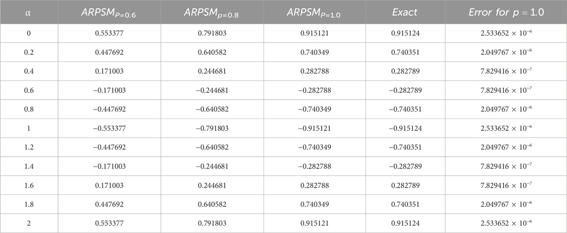
Table 1. ARPSM solution of problem 1 for different values of fractional order p for β = 0.01.

3.1.2 Anatomy Problem 2 using ARPSM

Consider the following time-fractional KdV equation:

$\begin{array}{cc}\hfill & D_{\beta }^p\varphi \left(\alpha ,\beta \right)+\varphi \left(\alpha ,\beta \right)\frac{\partial \varphi \left(\alpha ,\beta \right)}{\partial \alpha }-\frac{{\partial }^3\varphi \left(\alpha ,\beta \right)}{\partial {\alpha }^3}=0,\text{\hspace{0.17em}where\hspace{0.17em}}0<p\le 1\hfill \end{array}(49)$

having the following IC’s:

$\begin{array}{c}\hfill \varphi \left(\alpha ,0\right)=2\alpha .\end{array}(50)$

and exact solution

$\begin{array}{c}\hfill \varphi \left(\alpha ,\beta \right)=\frac{2\alpha }{2\beta +1}.\end{array}(51)$

Equation 50 is used in conjunction with AT applied to Eq. 49 to get:

$\begin{array}{c}\hfill \varphi \left(\alpha ,s\right)-\frac{2\alpha }{s^2}+\frac{1}{s^p}{A}_{\beta }\left[A_{\beta }^{-1}\varphi \left(\alpha ,\beta \right)\times \frac{\partial A_{\beta }^{-1}\varphi \left(\alpha ,\beta \right)}{\partial \alpha }\right]-\frac{1}{s^p}\left[\frac{{\partial }^3\varphi \left(\alpha ,\beta \right)}{\partial {\alpha }^3}\right]=0,\end{array}(52)$

Accordingly, the terms of the series that have been kth truncated are

$\begin{array}{c}\hfill \varphi \left(\alpha ,s\right)=\frac{2\alpha }{s^2}+{\displaystyle \sum _{r=1}^k}\frac{f_r\left(\alpha ,s\right)}{s^{rp+1}},r=\mathrm{1,2,3,4}\cdots .\end{array}(53)$

Aboodh residual functions (ARFs) are

$\begin{array}{c}\hfill A_{\beta }Res\left(\alpha ,s\right)=\varphi \left(\alpha ,s\right)-\frac{2\alpha }{s^2}+\frac{1}{s^p}{A}_{\beta }\left[A_{\beta }^{-1}\varphi \left(\alpha ,\beta \right)\times \frac{\partial A_{\beta }^{-1}\varphi \left(\alpha ,\beta \right)}{\partial \alpha }\right]-\frac{1}{s^p}\left[\frac{{\partial }^3\varphi \left(\alpha ,\beta \right)}{\partial {\alpha }^3}\right]=0,\end{array}(54)$

and the kth-LRFs as:

$\begin{array}{c}\hfill A_{\beta }Re{s}_k\left(\alpha ,\eta ,s\right)={\varphi }_k\left(\alpha ,s\right)-\frac{2\alpha }{s^2}+\frac{1}{s^p}{A}_{\beta }\left[A_{\beta }^{-1}{\varphi }_k\left(\alpha ,\beta \right)\times \frac{\partial A_{\beta }^{-1}{\varphi }_k\left(\alpha ,\beta \right)}{\partial \alpha }\right]-\frac{1}{s^p}\left[\frac{{\partial }^3{\varphi }_k\left(\alpha ,\beta \right)}{\partial {\alpha }^3}\right]=0,\end{array}(55)$

To find f_r (α, s) now r = 1, 2, 3, …. We multiply the resultant equation by s^rp+1, replace the rth-truncated series Eq. 53 into the rth-ARF Eq. 55, and solve the relation lim_s→∞(s^rp+1) iteratively. r = 1, 2, 3, ⋯, and A_βRes_ϕ,r (α, s)) = 0. Here are the first few of terms:

$\begin{array}{c}\hfill f_1\left(\alpha ,\eta ,s\right)=-4\alpha ,\end{array}(56)$

$\begin{array}{cc}\hfill & f_2\left(\alpha ,\eta ,s\right)=16\alpha ,\hfill \end{array}(57)$

$\begin{array}{cc}\hfill & f_3\left(\alpha ,\eta ,s\right)=-\frac{16\alpha \mathrm{\Gamma }\left(2p+1\right)}{\mathrm{\Gamma }{\left(p+1\right)}^2}-64\alpha ,\hfill \end{array}(58)$

and so on.

Equation 53 is used to get the values of f_r (α, s) for r = 1, 2, 3, … ,.

$\begin{array}{c}\hfill \varphi \left(\alpha ,s\right)=-\frac{4\alpha }{s^{p+1}}+\frac{16\alpha }{s^{2p+1}}+\frac{-\frac{16\alpha \mathrm{\Gamma }\left(2p+1\right)}{\mathrm{\Gamma }{\left(p+1\right)}^2}-64\alpha }{s^{3p+1}}+\frac{2\alpha }{s^2}+\cdots .\end{array}(59)$

When we use Aboodh’s inverse transform, we get

$\begin{array}{c}\hfill \varphi \left(\alpha ,\beta \right)=\frac{16\alpha {\beta }^{2p}}{\mathrm{\Gamma }\left(2p+1\right)}-\frac{64\alpha {\beta }^{3p}}{\mathrm{\Gamma }\left(3p+1\right)}-\frac{16\alpha {\beta }^{3p}\mathrm{\Gamma }\left(2p+1\right)}{\mathrm{\Gamma }{\left(p+1\right)}^2\mathrm{\Gamma }\left(3p+1\right)}-\frac{4\alpha {\beta }^p}{\mathrm{\Gamma }\left(p+1\right)}+2\alpha +\cdots .\end{array}(60)$

For the problem (49), the approximation (60) using ARPSM is compared with the exact solution (51) for the integer case, i.e., for p = 1 as illustrated in Figure 2. It can be seen from this figure how consistent the two solutions are with each other, which confirms the accuracy of the approximate solution (60). The approximation (60) is numerically examined against the fractional parameter p as shown in Figure 3. It is observed that the fractional parameter p strongly affects the profile of these waves; the wave amplitude decays with growing pit. Moreover, we estimated the absolute error compared to the exact solution for the integer case, as seen in Table 2. One can see from the comparison results that the error is minimal, and this enhances the high accuracy and stability of the inferred approximations.

Figure 2

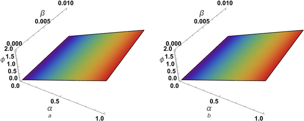
Figure 2. This figure shows: (A) approximate solution (60) via ARPSM at p =1 (B) the exact solution (51) of problem 2 for β =0.01.

Figure 3

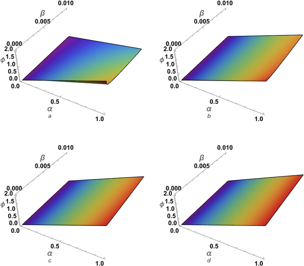
Figure 3. The approximation (60) using ARPSM for the problem (49) is numerically analyzed against the fractional parameter p for β =0.01: (A) p =0.3, (B) p =0.5, (C) p =0.7, and (D) p =1.

Table 2

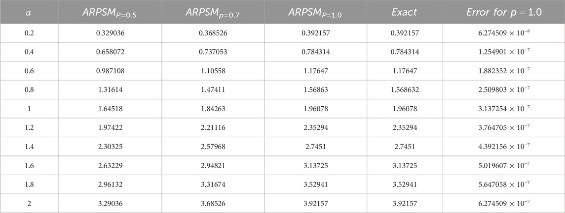
Table 2. ARPSM solution of problem 2 for different values of fractional order p for β = 0.01.

3.2 An overview of the aboodh iterative transform technique

Consider the general PDE of space-time fractional order.

$D_{\beta }^p\varphi \left(\alpha ,\beta \right)=\mathrm{\Phi }\left(\varphi \left(\alpha ,\beta \right),D_{\alpha }^{\beta }\varphi \left(\alpha ,\beta \right),D_{\alpha }^{2\beta }\varphi \left(\alpha ,\beta \right),D_{\alpha }^{3\beta }\varphi \left(\alpha ,\beta \right)\right),0<p,\beta \le 1,(61)$

Having the following IC’s.

${\varphi }^{\left(k\right)}\left(\alpha ,0\right)=h_k,k=\mathrm{0,1,2},\dots ,m-1,(62)$

Determine the unknown function denoted as ϕ(α, β), while $\mathrm{\Phi }\left(\varphi (\alpha ,\beta ),D_{\alpha }^{\beta }\varphi (\alpha ,\beta ),D_{\alpha }^{2\beta }\varphi (\alpha ,\beta ),D_{\alpha }^{3\beta }\varphi (\alpha ,\beta )\right)$ may be a nonlinear operator or linear of $\varphi (\alpha ,\beta ),D_{\alpha }^{\beta }\varphi (\alpha ,\beta ),D_{\alpha }^{2\beta }\varphi (\alpha ,\beta )$ and$D_{\alpha }^{3\beta }\varphi (\alpha ,\beta )$. Using the AT on both sides of Eq. (61), gives the following equation; for convenience, we represent ϕ(α, β) with ϕ.

$A\left[\varphi \left(\alpha ,\beta \right)\right]=\frac{1}{s^p}\left({\displaystyle \sum _{k=0}^{m-1}}\frac{{\varphi }^{\left(k\right)}\left(\alpha ,0\right)}{s^{2-p+k}}+A\left[\mathrm{\Phi }\left(\varphi \left(\alpha ,\beta \right),D_{\alpha }^{\beta }\varphi \left(\alpha ,\beta \right),D_{\alpha }^{2\beta }\varphi \left(\alpha ,\beta \right),D_{\alpha }^{3\beta }\varphi \left(\alpha ,\beta \right)\right)\right]\right),(63)$

Solving this problem using the AIT yields:

$\varphi \left(\alpha ,\beta \right)=A^{-1}\left[\frac{1}{s^p}\left({\displaystyle \sum _{k=0}^{m-1}}\frac{{\varphi }^{\left(k\right)}\left(\alpha ,0\right)}{s^{2-p+k}}+A\left[\mathrm{\Phi }\left(\varphi \left(\alpha ,\beta \right),D_{\alpha }^{\beta }\varphi \left(\alpha ,\beta \right),D_{\alpha }^{2\beta }\varphi \left(\alpha ,\beta \right),D_{\alpha }^{3\beta }\varphi \left(\alpha ,\beta \right)\right)\right]\right)\right].(64)$

The solution obtained through the iterative Aboodh transform method is denoted by an infinite series.

$\varphi \left(\alpha ,\beta \right)={\displaystyle \sum _{i=0}^{\infty }}{\varphi }_i.(65)$

Since $\mathrm{\Phi }\left(\varphi ,D_{\alpha }^{\beta }\varphi ,D_{\alpha }^{2\beta }\varphi ,D_{\alpha }^{3\beta }\varphi \right)$ is either a nonlinear or linear operator which can be decomposed as follows:

$\begin{array}{cc}\hfill & \mathrm{\Phi }\left(\varphi ,D_{\alpha }^{\beta }\varphi ,D_{\alpha }^{2\beta }\varphi ,D_{\alpha }^{3\beta }\varphi \right)=\mathrm{\Phi }\left({\varphi }_0,D_{\alpha }^{\beta }{\varphi }_0,D_{\alpha }^{2\beta }{\varphi }_0,D_{\alpha }^{3\beta }{\varphi }_0\right)\hfill \\ \hfill & +{\displaystyle \sum _{i=0}^{\infty }}(\mathrm{\Phi }\left({\displaystyle \sum _{k=0}^i}\left({\varphi }_k,D_{\alpha }^{\beta }{\varphi }_k,D_{\alpha }^{2\beta }{\varphi }_k,D_{\alpha }^{3\beta }{\varphi }_k\right)\right)-\mathrm{\Phi }\left({\displaystyle \sum _{k=1}^{i-1}}\left({\varphi }_k,D_{\alpha }^{\beta }{\varphi }_k,D_{\alpha }^{2\beta }{\varphi }_k,D_{\alpha }^{3\beta }{\varphi }_k\right)\right)).\hfill \end{array}(66)$

By substituting Eqs 65, 66 into Eq. 64, the subsequent equation is obtained.

$\begin{array}{cc}\hfill & {\displaystyle \sum _{i=0}^{\infty }}{\varphi }_i\left(\alpha ,\beta \right)=A^{-1}\left[\frac{1}{s^p}\left({\displaystyle \sum _{k=0}^{m-1}}\frac{{\varphi }^{\left(k\right)}\left(\alpha ,0\right)}{s^{2-p+k}}+A\left[\mathrm{\Phi }\left({\varphi }_0,D_{\alpha }^{\beta }{\varphi }_0,D_{\alpha }^{2\beta }{\varphi }_0,D_{\alpha }^{3\beta }{\varphi }_0\right)\right]\right)\right]\hfill \\ \hfill & +A^{-1}\left[\frac{1}{s^p}\left(A\left[{\displaystyle \sum _{i=0}^{\infty }}\left(\mathrm{\Phi }{\displaystyle \sum _{k=0}^i}\left({\varphi }_k,D_{\alpha }^{\beta }{\varphi }_k,D_{\alpha }^{2\beta }{\varphi }_k,D_{\alpha }^{3\beta }{\varphi }_k\right)\right)\right]\right)\right]\hfill \\ \hfill & -A^{-1}\left[\frac{1}{s^p}\left(A\left[\left(\mathrm{\Phi }{\displaystyle \sum _{k=1}^{i-1}}\left({\varphi }_k,D_{\alpha }^{\beta }{\varphi }_k,D_{\alpha }^{2\beta }{\varphi }_k,D_{\alpha }^{3\beta }{\varphi }_k\right)\right)\right]\right)\right]\hfill \end{array}(67)$

$\begin{array}{cc}\hfill & {\varphi }_0\left(\alpha ,\beta \right)=A^{-1}\left[\frac{1}{s^p}\left({\displaystyle \sum _{k=0}^{m-1}}\frac{{\varphi }^{\left(k\right)}\left(\alpha ,0\right)}{s^{2-p+k}}\right)\right],\hfill \\ \hfill & {\varphi }_1\left(\alpha ,\beta \right)=A^{-1}\left[\frac{1}{s^p}\left(A\left[\mathrm{\Phi }\left({\varphi }_0,D_{\alpha }^{\beta }{\varphi }_0,D_{\alpha }^{2\beta }{\varphi }_0,D_{\alpha }^{3\beta }{\varphi }_0\right)\right]\right)\right],\hfill \\ \hfill ⋮\\ \hfill & {\varphi }_{m+1}\left(\alpha ,\beta \right)=A^{-1}\left[\frac{1}{s^p}\left(A\left[{\displaystyle \sum _{i=0}^{\infty }}\left(\mathrm{\Phi }{\displaystyle \sum _{k=0}^i}\left({\varphi }_k,D_{\alpha }^{\beta }{\varphi }_k,D_{\alpha }^{2\beta }{\varphi }_k,D_{\alpha }^{3\beta }{\varphi }_k\right)\right)\right]\right)\right]\hfill \\ \hfill & -A^{-1}\left[\frac{1}{s^p}\left(A\left[\left(\mathrm{\Phi }{\displaystyle \sum _{k=1}^{i-1}}\left({\varphi }_k,D_{\alpha }^{\beta }{\varphi }_k,D_{\alpha }^{2\beta }{\varphi }_k,D_{\alpha }^{3\beta }{\varphi }_k\right)\right)\right]\right)\right],m=\mathrm{1,2},\cdots .\hfill \end{array}(68)$

Eq. 61 may be expressed as follows, which gives the m-term analytically approximate solution:

$\varphi \left(\alpha ,\beta \right)={\displaystyle \sum _{i=0}^{m-1}}{\varphi }_i.(69)$

3.2.1 Anatomy problem 1 using ATIM

Consider the following time-fractional Burger’s equation:

$\begin{array}{cc}\hfill & D_{\beta }^p\varphi \left(\alpha ,\beta \right)=\frac{{\partial }^2\varphi \left(\alpha ,\beta \right)}{\partial {\beta }^2}+\varphi \left(\alpha ,\beta \right),\text{\hspace{0.17em}where\hspace{0.17em}}0<p\le 1\hfill \end{array}(70)$

having the following IC’s:

$\begin{array}{c}\hfill \varphi \left(\alpha ,0\right)=\cos \left(\pi \alpha \right),\end{array}(71)$

and exact solution

$\begin{array}{c}\hfill \varphi \left(\alpha ,\beta \right)=e^{-\left({\pi }^2-1\right)\beta }\cos \left(\pi \alpha \right).\end{array}(72)$

By applying the AT on each side of Eq. 70, we arrive at the following result:

$A\left[D_{\beta }^p\varphi \left(\alpha ,\beta \right)\right]=\frac{1}{s^p}\left({\displaystyle \sum _{k=0}^{m-1}}\frac{{\varphi }^{\left(k\right)}\left(\alpha ,\eta ,0\right)}{s^{2-p+k}}+A\left[\frac{{\partial }^2\varphi \left(\alpha ,\beta \right)}{\partial {\beta }^2}+\varphi \left(\alpha ,\beta \right)\right]\right),(73)$

When we apply the AIT to both sides of Eq. 73, we get:

$\varphi \left(\alpha ,\beta \right)=A^{-1}\left[\frac{1}{s^p}\left({\displaystyle \sum _{k=0}^{m-1}}\frac{{\varphi }^{\left(k\right)}\left(\alpha ,\eta ,0\right)}{s^{2-p+k}}+A\left[\frac{{\partial }^2\varphi \left(\alpha ,\beta \right)}{\partial {\beta }^2}+\varphi \left(\alpha ,\beta \right)\right]\right)\right].(74)$

The equation that we get by iteratively applying the AT is given as:

$\begin{array}{cc}\hfill {\varphi }_0\left(\alpha ,\beta \right)=& A^{-1}\left[\frac{1}{s^p}\left({\displaystyle \sum _{k=0}^{m-1}}\frac{{\varphi }^{\left(k\right)}\left(\alpha ,\eta ,0\right)}{s^{2-p+k}}\right)\right]\hfill \\ \hfill & =A^{-1}\left[\frac{\varphi \left(\alpha ,\eta ,0\right)}{s^2}\right]\hfill \\ \hfill & =\cos \left(\pi \alpha \right),\hfill \end{array}$

By substituting the RL integral into Eq. 70, we obtained the equivalent form.

$\begin{array}{c}\hfill \varphi \left(\alpha ,\beta \right)=\cos \left(\pi \alpha \right)-A\left[\frac{{\partial }^2\varphi \left(\alpha ,\beta \right)}{\partial {\beta }^2}+\varphi \left(\alpha ,\beta \right)\right].\end{array}(75)$

Here are a few terms that are obtained using the ATIM procedure:

$\begin{array}{cc}\hfill & {\varphi }_0\left(\alpha ,\beta \right)=\cos \left(\pi \alpha \right),\hfill \\ \hfill & {\varphi }_1\left(\alpha ,\beta \right)=-\frac{\left({\pi }^2-1\right){\beta }^p\cos \left(\pi \alpha \right)}{\mathrm{\Gamma }\left(p+1\right)},\hfill \\ \hfill & {\varphi }_2\left(\alpha ,\beta \right)=\frac{{\left({\pi }^2-1\right)}^2{\beta }^{2p}\cos \left(\pi \alpha \right)}{\mathrm{\Gamma }\left(2p+1\right)},\hfill \\ \hfill & {\varphi }_3\left(\alpha ,\beta \right)=-\frac{{\left({\pi }^2-1\right)}^3{\beta }^{3p}\cos \left(\pi \alpha \right)}{\mathrm{\Gamma }\left(3p+1\right)},\hfill \end{array}(76)$

The ultimate ATIM solution is given as:

$\begin{array}{c}\hfill \varphi \left(\alpha ,\beta \right)={\varphi }_0\left(\alpha ,\beta \right)+{\varphi }_1\left(\alpha ,\beta \right)+{\varphi }_2\left(\alpha ,\beta \right)+{\varphi }_3\left(\alpha ,\beta \right)+\cdots .\end{array}(77)$

$\begin{array}{c}\hfill \varphi \left(\alpha ,\beta \right)=\frac{{\left({\pi }^2-1\right)}^2{\beta }^{2p}\cos \left(\pi \alpha \right)}{\mathrm{\Gamma }\left(2p+1\right)}-\frac{{\left({\pi }^2-1\right)}^3{\beta }^{3p}\cos \left(\pi \alpha \right)}{\mathrm{\Gamma }\left(3p+1\right)}-\frac{\left({\pi }^2-1\right){\beta }^p\cos \left(\pi \alpha \right)}{\mathrm{\Gamma }\left(p+1\right)}+\cos \left(\pi \alpha \right)+\cdots .\end{array}(78)$

The approximation (78) using ATIM for the problem (70) is numerically investigated as demonstrated in Figure 4. It is shown that the fractional parameter p has a strong affect on the profile solution. Moreover, we estimated the absolute error compared to the exact solution (72) for the integer case, as shown in Table 3. It is observed from the comparison results that the error is minimal, and this enhances the high accuracy and stability of the inferred approximations.

Figure 4

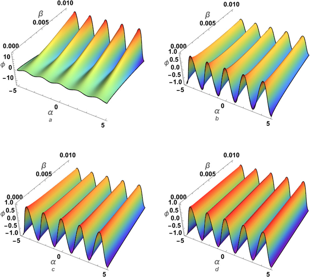
Figure 4. The approximation (78) using ATIM for the problem (70) is numerically analyzed against the fractional parameter p for β =0.01: (A) p =0.3, (B) p =0.5, (C) p =0.7, and (D) p =1.

Table 3

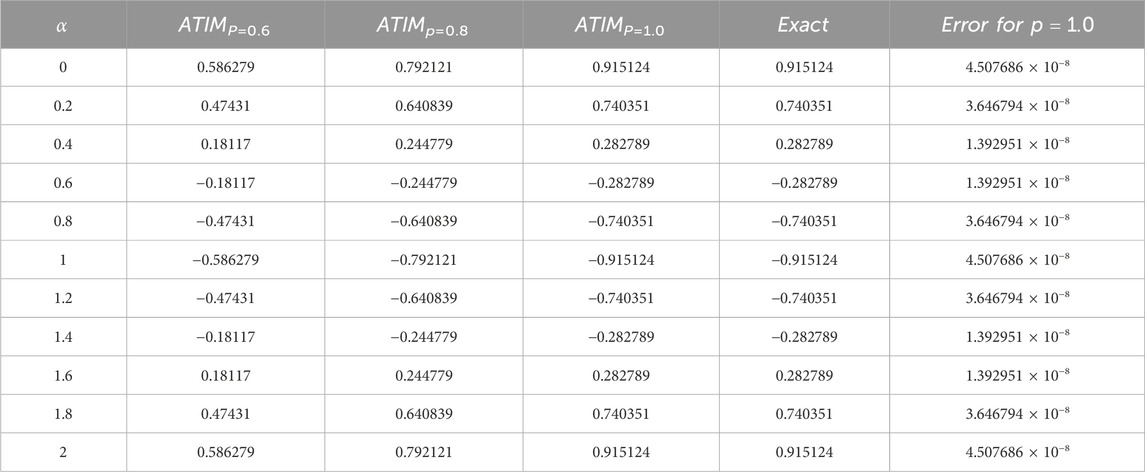
Table 3. ATIM solution of problem 1 for different values of fractional order p for β = 0.01.

3.2.2 Anatomy problem 2 using ATIM

Consider the following time-fractional KdV equation:

$\begin{array}{cc}\hfill & D_{\beta }^p\varphi \left(\alpha ,\beta \right)=-\varphi \left(\alpha ,\beta \right)\frac{\partial \varphi \left(\alpha ,\beta \right)}{\partial \alpha }+\frac{{\partial }^3\varphi \left(\alpha ,\beta \right)}{\partial {\alpha }^3},\text{\hspace{0.17em}where\hspace{0.17em}}0<p\le 1\hfill \end{array}(79)$

having the following IC’s:

$\begin{array}{c}\hfill \varphi \left(\alpha ,0\right)=2\alpha ,\end{array}(80)$

and the exact solution

$\begin{array}{c}\hfill \varphi \left(\alpha ,\beta \right)=\frac{2\alpha }{2\beta +1}.\end{array}(81)$

After executing the AT on each side of Eq. 79, we obtain:

$\begin{array}{c}\hfill A\left[D_{\beta }^p\varphi \left(\alpha ,\beta \right)\right]=\frac{1}{s^p}\left({\displaystyle \sum _{k=0}^{m-1}}\frac{{\varphi }^{\left(k\right)}\left(\alpha ,\eta ,0\right)}{s^{2-p+k}}+A\left[-\varphi \left(\alpha ,\beta \right)\frac{\partial \varphi \left(\alpha ,\beta \right)}{\partial \alpha }+\frac{{\partial }^3\varphi \left(\alpha ,\beta \right)}{\partial {\alpha }^3}\right]\right),\end{array}(82)$

Equation that results from applying the AIT to Eq. 82 is:

$\begin{array}{c}\hfill \varphi \left(\alpha ,\eta ,\beta \right)=A^{-1}\left[\frac{1}{s^p}\left({\displaystyle \sum _{k=0}^{m-1}}\frac{{\varphi }^{\left(k\right)}\left(\alpha ,\eta ,0\right)}{s^{2-p+k}}+A\left[-\varphi \left(\alpha ,\beta \right)\frac{\partial \varphi \left(\alpha ,\beta \right)}{\partial \alpha }+\frac{{\partial }^3\varphi \left(\alpha ,\beta \right)}{\partial {\alpha }^3}\right]\right)\right].\end{array}(83)$

This equation is obtained by using the iterative process of the AT:

$\begin{array}{cc}\hfill {\varphi }_0\left(\alpha ,\eta ,\beta \right)=& A^{-1}\left[\frac{1}{s^p}\left({\displaystyle \sum _{k=0}^{m-1}}\frac{{\varphi }^{\left(k\right)}\left(\alpha ,0\right)}{s^{2-p+k}}\right)\right]\hfill \\ \hfill & =A^{-1}\left[\frac{\varphi \left(\alpha ,0\right)}{s^2}\right]\hfill \\ \hfill & =2\alpha ,\hfill \end{array}$

Equation 49 yields the equivalent form when the RL integral is applied.

$\begin{array}{c}\hfill \varphi \left(\alpha ,\beta \right)=2\alpha -A\left[-\varphi \left(\alpha ,\beta \right)\frac{\partial \varphi \left(\alpha ,\beta \right)}{\partial \alpha }+\frac{{\partial }^3\varphi \left(\alpha ,\beta \right)}{\partial {\alpha }^3}\right].\end{array}(84)$

We get these terms from the ATIM procedure.

$\begin{array}{cc}\hfill & {\varphi }_0\left(\alpha ,\beta \right)=2\alpha ,\hfill \\ \hfill & {\varphi }_1\left(\alpha ,\beta \right)=-\frac{4\alpha {\beta }^p}{\mathrm{\Gamma }\left(p+1\right)},\hfill \\ \hfill & {\varphi }_2\left(\alpha ,\beta \right)=16\alpha {\beta }^{2p}\left(\frac{1}{\mathrm{\Gamma }\left(2p+1\right)}-\frac{4^p{\beta }^p\mathrm{\Gamma }\left(p+\frac{1}{2}\right)}{\sqrt{\pi }\mathrm{\Gamma }\left(p+1\right)\mathrm{\Gamma }\left(3p+1\right)}\right),\hfill \\ \hfill & {\varphi }_3\left(\alpha \beta \right)=\left(128\alpha {\beta }^{4p}\left(\sqrt{\pi }\mathrm{\Gamma }{\left(3p+1\right)}^2\mathrm{\Gamma }\left(5p+1\right)(\mathrm{\Gamma }\left(p\right)\mathrm{\Gamma }\left(p+1\right)\mathrm{\Gamma }\left(3p+1\right)-2{\beta }^p\mathrm{\Gamma }\left(2p\right)\mathrm{\Gamma }\left(2p+1\right))\right.\right.\hfill \\ \hfill & -8{\beta }^p\mathrm{\Gamma }\left(4p\right)\left(4^p{\beta }^{2p}\mathrm{\Gamma }\left(p+\frac{1}{2}\right)\mathrm{\Gamma }{\left(2p+1\right)}^2\mathrm{\Gamma }\left(4p+1\right)-2\sqrt{\pi }{\beta }^p\mathrm{\Gamma }\left(p+1\right)\mathrm{\Gamma }\left(2p+1\right)\mathrm{\Gamma }\left(3p+1\right)\mathrm{\Gamma }\left(4p+1\right)\right.\hfill \\ \hfill & \left.\left.\left.+16^p\mathrm{\Gamma }{\left(p+1\right)}^3\mathrm{\Gamma }\left(2p+\frac{1}{2}\right)\mathrm{\Gamma }{\left(3p+1\right)}^2\right)\right)\right)/\left(\sqrt{\pi }\mathrm{\Gamma }\left(p\right)\mathrm{\Gamma }{\left(p+1\right)}^2\mathrm{\Gamma }\left(2p+1\right)\mathrm{\Gamma }{\left(3p+1\right)}^2\mathrm{\Gamma }\left(4p+1\right)\mathrm{\Gamma }\left(5p+1\right)\right),\hfill \end{array}(85)$

The ultimate result of the ATIM algorithm is given as:

$\begin{array}{c}\hfill \varphi \left(\alpha ,\beta \right)={\varphi }_0\left(\alpha ,\beta \right)+{\varphi }_1\left(\alpha ,\beta \right)+{\varphi }_2\left(\alpha ,\beta \right)+{\varphi }_3\left(\alpha ,\beta \right)+\cdots \end{array}(86)$

$\begin{array}{cc}\hfill & \varphi \left(\alpha ,\beta \right)=2\alpha -\frac{4\alpha {\beta }^p}{\mathrm{\Gamma }\left(p+1\right)}+16\alpha {\beta }^{2p}\left(\frac{1}{\mathrm{\Gamma }\left(2p+1\right)}-\frac{4^p{\beta }^p\mathrm{\Gamma }\left(p+\frac{1}{2}\right)}{\sqrt{\pi }\mathrm{\Gamma }\left(p+1\right)\mathrm{\Gamma }\left(3p+1\right)}\right)\hfill \\ \hfill & +\left(128\alpha {\beta }^{4p}\left(\sqrt{\pi }\mathrm{\Gamma }{\left(3p+1\right)}^2\mathrm{\Gamma }\left(5p+1\right)\left(\mathrm{\Gamma }\left(p\right)\mathrm{\Gamma }\left(p+1\right)\mathrm{\Gamma }\left(3p+1\right)-2{\beta }^p\mathrm{\Gamma }\left(2p\right)\mathrm{\Gamma }\left(2p+1\right)\right)\right.\right.\hfill \\ \hfill & -8{\beta }^p\mathrm{\Gamma }\left(4p\right)\left(4^p{\beta }^{2p}\mathrm{\Gamma }\left(p+\frac{1}{2}\right)\mathrm{\Gamma }{\left(2p+1\right)}^2\mathrm{\Gamma }\left(4p+1\right)-2\sqrt{\pi }{\beta }^p\mathrm{\Gamma }\left(p+1\right)\mathrm{\Gamma }\times \left(2p+1\right)\mathrm{\Gamma }\left(3p+1\right)\mathrm{\Gamma }\left(4p+1\right)\right.\hfill \\ \hfill & \left.\left.\left.+16^p\mathrm{\Gamma }{\left(p+1\right)}^3\mathrm{\Gamma }\left(2p+\frac{1}{2}\right)\mathrm{\Gamma }{\left(3p+1\right)}^2\right)\right)\right)/\left(\sqrt{\pi }\mathrm{\Gamma }\left(p\right)\mathrm{\Gamma }{\left(p+1\right)}^2\mathrm{\Gamma }\left(2p+1\right)\mathrm{\Gamma }{\left(3p+1\right)}^2\mathrm{\Gamma }\left(4p+1\right)\mathrm{\Gamma }\left(5p+1\right)\right).\hfill \end{array}(87)$

The approximation (87) using ATIM for the problem (79) is compared with the exact solution (81) for the integer case, i.e., for p = 1 as demonstrated in Figure 5. The obtained results demonstrate a good matching between the two solutions, which confirms the accuracy of the approximate solution (87). Additionally, the approximation (87) is numerically examined against the fractional parameter p, as shown in Figure 6. It is found that the fractional parameter p has a substantial impact on the wave profile. Moreover, we estimated the absolute error compared to the exact solution for the integer case, as seen in Table 4. One can see from the comparison results that the error is minimal, and this enhances the high accuracy and stability of the inferred approximations. Furthermore, we made a numerical comparison between the approximate solutions deduced using ATIM and APRSM, for example, 1 and 2, as shown in Tables 5 and Table 6. It is clear from the comparison results that the approximate solutions are more accurate. Also, it is observed that ATIM is more accurate than APRSM. However, in general, both approaches are characterized by high accuracy and stability throughout the field of study.

Figure 5

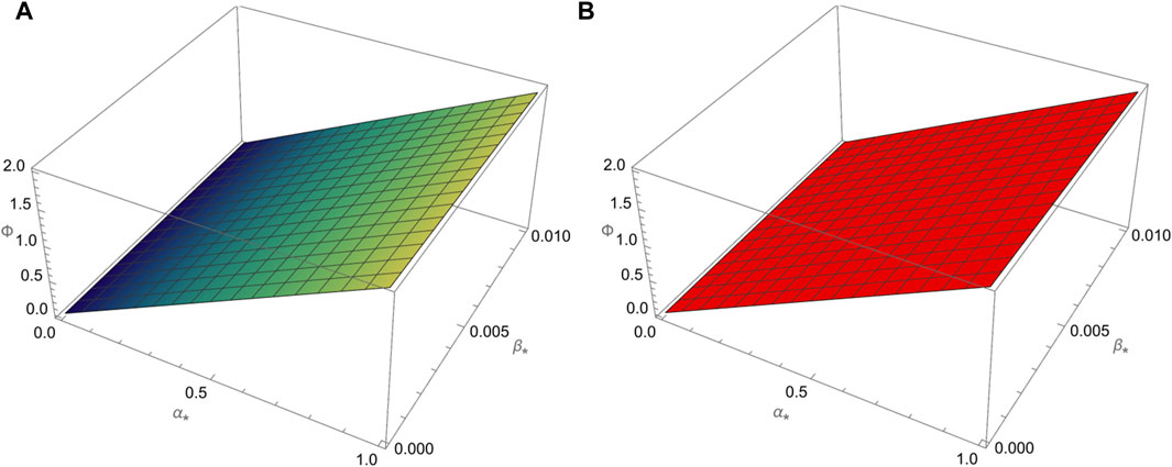
Figure 5. Here, we considered the comparison between (A) the approximate solution (87) via ATIM and (B) exact solution (81) of problem 2 for β =0.01.

Figure 6

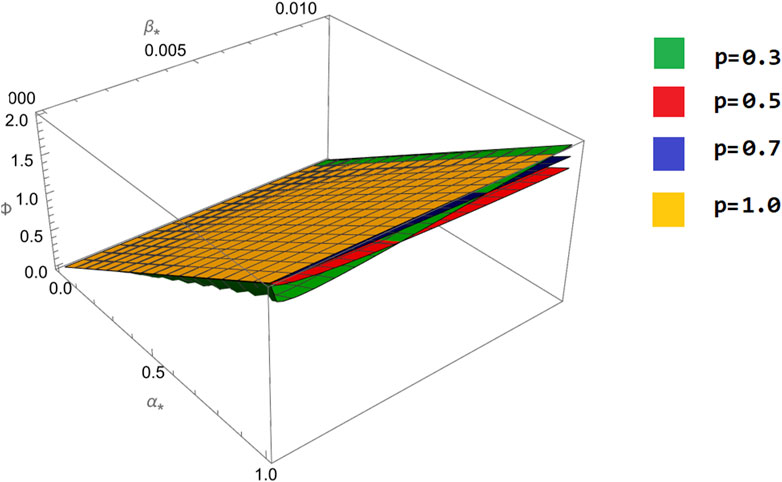
Figure 6. The approximation (87) using ATIM for the problem (79) is numerically analyzed against the fractional parameter p for β =0.01.

Table 4

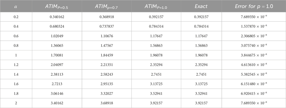
Table 4. ATIM solution of problem 2 for different values of fractional order p for β = 0.01.

Table 5

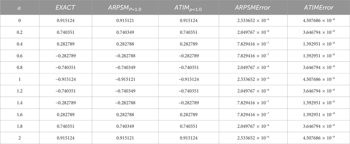
Table 5. An analysis of the absolute error between the ATIM and APRSM, for example, 1 at β = 0.01.

Table 6

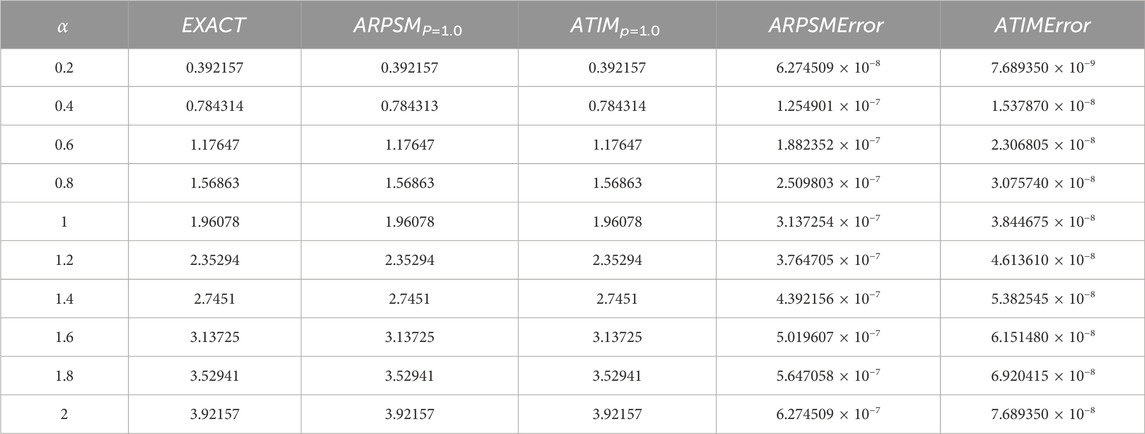
Table 6. An analysis of the absolute error between the ATIM and APRSM, for example, 2 at β = 0.01.

4 Conclusion

This paper has thoroughly examined the dynamics of fractional linear and nonlinear partial differential equations using advanced mathematical methods for solving them. The Aboodh Residual Power Series Method (ARPSM) and the Aboodh Transform Iteration Method (ATIM) are particularly effective in solving difficult equations accurately and insightfully. Including the Caputo operator, a key component of fractional calculus, has improved the accuracy and usefulness of the suggested techniques. This research has substantially contributed to the knowledge of fractional calculus applications in mathematical physics by comprehensively analyzing linear and nonlinear scenarios. These methods were applied to solve different examples of fractional differential equations, and some approximate solutions were derived and analyzed numerically to verify their accuracy and stability throughout the study domain. Moreover, the absolute error of these approximations compared to the exact solutions for the integer case was also estimated. The numerical results have proven the high accuracy and stability of the deduced approximations, which enhances the ability and efficiency of the used methods. The proven effectiveness of the ARPSM and ATIM indicates their ability to solve many issues across different scientific fields. This study enhances the approaches for solving fractional partial differential equations and paves the way for further inquiry and application in scientific and technical fields.

4.1 Future work

These methods are suitable for modeling many evolution equations in their fractional form that govern many nonlinear phenomena in different plasma systems. For example, these methods can analyze the KdV family [49–54] and the family of Kawahara-type equations (55)–(59), which describes solitary and periodic waves propagating with phase speed in a plasma. Moreover, these methods can be applied to analyze the family of nonlinear Schrödinger-type equations in their fractional form, which governs the propagation of nonlinear waves at group speed in a plasma [60–65].

Data availability statement

The original contributions presented in the study are included in the article/supplementary material, further inquiries can be directed to the corresponding authors.

Author contributions

SN: Funding acquisition, Investigation, Supervision, Writing–review and editing. WA: Data curation, Formal Analysis, Investigation, Visualization, Writing–review and editing. RS: Investigation, Methodology, Resources, Validation, Supervision, Writing–review and editing. AS: Software, Validation, Visualization, Writing–review and editing. SI: Investigation, Methodology, Project administration, Visualization, Writing–review and editing. SE-T: Formal Analysis, Investigation, Methodology, Resources, Software, Supervision, Validation, Writing–review and editing.

Funding

The author(s) declare financial support was received for the research, authorship, and/or publication of this article. The authors express their gratitude to Princess Nourah bint Abdulrahman University Researchers Supporting Project Number(PNURSP2024R157), Princess Nourah bint AbdulrahmanUniversity, Riyadh, Saudi Arabia. This work was supported by the Deanship of Scientific Research, Vice Presidency for Graduate Studies and Scientific Research, King Faisal University, Saudi Arabia (Grant No. 5903).

Acknowledgments

The authors express their gratitude to Princess Nourah bintAbdulrahman University Researchers Supporting Project Number(PNURSP2024R157), Princess Nourah bint AbdulrahmanUniversity, Riyadh, Saudi Arabia. This work was supported by the Deanship of Scientific Research, Vice Presidency for Graduate Studies and Scientific Research, King Faisal University, Saudi Arabia (Grant No. 5903).

Conflict of interest

The authors declare that the research was conducted in the absence of any commercial or financial relationships that could be construed as a potential conflict of interest.

Publisher’s note

All claims expressed in this article are solely those of the authors and do not necessarily represent those of their affiliated organizations, or those of the publisher, the editors and the reviewers. Any product that may be evaluated in this article, or claim that may be made by its manufacturer, is not guaranteed or endorsed by the publisher.

References

1. Podlubny I. Mathematics in science and engineering fractional differential equations: an introduction to fractional derivatives, fractional differential equations, to methods of their solution and some of their applications. Amsterdam, Netherlands: Elsevier (1999).

Google Scholar

2. Wang KL. New analysis methods for the coupled fractional nonlinear Hirota equation. Fractals (fractals) (2023) 31(09):1–14. doi:10.1142/s0218348x23501190

CrossRef Full Text | Google Scholar

3. Ozarslan R, Bas E, Baleanu D, Acay B. Fractional physical problems including wind-influenced projectile motion with Mittag-Leffler kernel. AIMS Math (2020) 5:467–81. doi:10.3934/math.2020031

CrossRef Full Text | Google Scholar

4. Wang KL. Investigation of the fractional kdv–zakharov–kuznetsov equation arising in plasma physics. Fractals (fractals) (2023) 31(7):1–15. doi:10.1142/s0218348x23500652

CrossRef Full Text | Google Scholar

5. Yavuz M, Ozdemir N. A different approach to the European option pricing model with new fractional operator. Math Model Nat Phenomena (2018) 13(1):12. doi:10.1051/mmnp/2018009

CrossRef Full Text | Google Scholar

6. Mukhtar S, Shah R, Noor S. The numerical investigation of a fractional-order multi-dimensional Model of Navier-Stokes equation via novel techniques. Symmetry (2022) 14(6):1102. doi:10.3390/sym14061102

CrossRef Full Text | Google Scholar

7. Wang KL. New solitary wave solutions and dynamical behaviors of the nonlinear fractional zakharov system. Qual Theor Dynamical Syst (2024) 23(3):98–20. doi:10.1007/s12346-024-00955-8

CrossRef Full Text | Google Scholar

8. Saad Alshehry A, Imran M, Khan A, Weera W. Fractional view analysis of kuramoto-sivashinsky equations with non-singular kernel operators. Symmetry (2022) 14(7):1463. doi:10.3390/sym14071463

CrossRef Full Text | Google Scholar

9. Wang KL. Novel approaches to fractional Klein-Gordon-Zakharov equation. Fractals (2023) 31(7):2350095. doi:10.1142/s0218348x23500950

CrossRef Full Text | Google Scholar

10. Wang KL. New promising and challenges of the fractional calogero-bogoyavlenskii-schiff equation. FRACTALS (fractals) (2023) 31(09):1–11. doi:10.1142/s0218348x23501104

CrossRef Full Text | Google Scholar

11. Srivastava HM, Khan H, Arif M. Some analytical and numerical investigation of a family of fractional-order Helmholtz equations in two space dimensions. Math Methods Appl Sci (2020) 43(1):199–212. doi:10.1002/mma.5846

CrossRef Full Text | Google Scholar

12. He HM, Peng JG, Li HY. Iterative approximation of fixed point problems and variational inequality problems on Hadamard manifolds. UPB Bull Ser A (2022) 84(1):25–36.

Google Scholar

13. Kai Y, Yin Z. On the Gaussian traveling wave solution to a special kind of Schrodinger equation with logarithmic nonlinearity. Mod Phys Lett B (2021) 36(02):2150543. doi:10.1142/S0217984921505436

CrossRef Full Text | Google Scholar

14. Kai Y, Chen S, Zhang K, Yin Z. Exact solutions and dynamic properties of a nonlinear fourth-order time-fractional partial differential equation. Waves in Random and Complex Media (2022) 1–12. doi:10.1080/17455030.2022.2044541

CrossRef Full Text | Google Scholar

15. Caputo M, Fabrizio M. A new definition of fractional derivative without singular kernel. Prog Fractional Differ Appl (2015) 1(2):73–85.

Google Scholar

16. Dokuyucu MA. A fractional order alcoholism model via Caputo-Fabrizio derivative. Aims Math (2020) 5(2):781–97. doi:10.3934/math.2020053

CrossRef Full Text | Google Scholar

17. Al-Sawalha MM, Khan A, Ababneh OY, Botmart T. Fractional view analysis of Kersten-Krasil,shchik coupled KdV-mKdV systems with non-singular kernel derivatives. AIMS Math (2022) 7:18334–59. doi:10.3934/math.20221010

CrossRef Full Text | Google Scholar

18. Higazy M, Alyami MA. New Caputo-Fabrizio fractional order SEIASqEqHR model for COVID-19 epidemic transmission with genetic algorithm based control strategy. Alexandria Eng J (2020) 59(6):4719–36. doi:10.1016/j.aej.2020.08.034

CrossRef Full Text | Google Scholar

19. Cai X, Tang R, Zhou H, Li Q, Ma S, Wang D, et al. Dynamically controlling terahertz wavefronts with cascaded metasurfaces. Adv Photon (2021) 3(3):036003. doi:10.1117/1.AP.3.3.036003

CrossRef Full Text | Google Scholar

20. Bai X, He Y, Xu M. Low-thrust reconfiguration strategy and optimization for formation flying using Jordan normal form. IEEE Trans Aerospace Electron Syst (2021) 57(5):3279–95. doi:10.1109/TAES.2021.3074204

CrossRef Full Text | Google Scholar

21. Zhou X, Liu X, Zhang G, Jia L, Wang X, Zhao Z. An iterative threshold algorithm of log-sum regularization for sparse problem. IEEE Trans Circuits Syst Video Tech (2023) 33(9):4728–40. doi:10.1109/TCSVT.2023.3247944

CrossRef Full Text | Google Scholar

22. Wang R, Feng Q, Ji J. The discrete convolution for fractional cosine-sine series and its application in convolution equations. AIMS Math (2024) 9(2):2641–56. doi:10.3934/math.2024130

CrossRef Full Text | Google Scholar

23. Guo C, Hu J, Hao J, Celikovsky S, Hu X. Fixed-time safe tracking control of uncertain high-order nonlinear pure-feedback systems via unified transformation functions. Kybernetika (2023) 59(3):342–64. doi:10.14736/kyb-2023-3-0342

CrossRef Full Text | Google Scholar

24. Schiff JL. The Laplace transform: theory and applications. Berlin, Germany: Springer Science and Business Media (1999).

Google Scholar

25. Watugala GK. Sumudu transform-a new integral transform to solve differential equations and control engineering problems. In: Control 92: enhancing Australia’s productivity through automation, control and instrumentation; preprints of papers. Australia: Barton, ACT: Institution of Engineers (1992). p. 245–59.

Google Scholar

26. Elzaki TM, Ezaki SM. Application of new transform “Elzaki transform” to partial differential equations. Glob J Pure Appl Math (2011) 7(1):65–70.

Google Scholar

27. Aboodh KS. Application of new transform “Aboodh Transform” to partial differential equations. Glob J Pure Appl Math (2014) 10(2):249–54.

Google Scholar

28. Arqub OA. Series solution of fuzzy differential equations under strongly generalized differentiability. J Adv Res Appl Math (2013) 5(1):31–52. doi:10.5373/jaram.1447.051912

CrossRef Full Text | Google Scholar

29. Abu Arqub O, Abo-Hammour Z, Al-Badarneh R, Momani S. A reliable analytical method for solving higher-order initial value problems. Discrete Dyn Nat Soc (2013) 2013:1–12. doi:10.1155/2013/673829

CrossRef Full Text | Google Scholar

30. Arqub OA, El-Ajou A, Zhour ZA, Momani S. Multiple solutions of nonlinear boundary value problems of fractional order: a new analytic iterative technique. Entropy (2014) 16(1):471–93. doi:10.3390/e16010471

CrossRef Full Text | Google Scholar

31. El-Ajou A, Arqub OA, Momani S. Approximate analytical solution of the nonlinear fractional KdV-Burgers equation: a new iterative algorithm. J Comput Phys (2015) 293:81–95. doi:10.1016/j.jcp.2014.08.004

CrossRef Full Text | Google Scholar

32. Xu F, Gao Y, Yang X, Zhang H. Construction of fractional power series solutions to fractional Boussinesq equations using residual power series method. Math Probl Eng (2016) 2016:1–15. doi:10.1155/2016/5492535

CrossRef Full Text | Google Scholar

33. Zhang J, Wei Z, Li L, Zhou C. Least-squares residual power series method for the time-fractional differential equations. Complexity (2019) 2019:1–15. doi:10.1155/2019/6159024

CrossRef Full Text | Google Scholar

34. Alderremy AA, Iqbal N, Aly S, Nonlaopon K. Fractional series solution construction for nonlinear fractional reaction-diffusion brusselator model utilizing Laplace residual power series. Symmetry (2022) 14(9):1944. doi:10.3390/sym14091944

CrossRef Full Text | Google Scholar

35. Jaradat I, Alquran M, Al-Khaled K. An analytical study of physical models with inherited temporal and spatial memory. The Eur Phys J Plus (2018) 133:162–11. doi:10.1140/epjp/i2018-12007-1

CrossRef Full Text | Google Scholar

36. Alquran M, Al-Khaled K, Sivasundaram S, Jaradat HM. Mathematical and numerical study of existence of bifurcations of the generalized fractional Burgers-Huxley equation. Nonlinear Stud (2017) 24(1):235–44.

Google Scholar

37. Guo C, Hu J, Wu Y, Celikovsky S. Non-Singular fixed-time tracking control of uncertain nonlinear pure-feedback systems with practical state constraints. IEEE Trans Circuits Syst Regular Pap (2023) 70(9):3746–58. doi:10.1109/TCSI.2023.3291700

CrossRef Full Text | Google Scholar

38. Yasmin H, Aljahdaly NH, Saeed AM, Shah R. Investigating symmetric soliton solutions for the fractional coupled konno-onno system using improved versions of a novel analytical technique. Mathematics (2023) 11(12):2686. doi:10.3390/math11122686

CrossRef Full Text | Google Scholar

39. Ojo GO, Mahmudov NI. Aboodh transform iterative method for spatial diffusion of a biological population with fractional-order. Mathematics (2021) 9(2):155. doi:10.3390/math9020155

CrossRef Full Text | Google Scholar

40. Awuya MA, Ojo GO, Mahmudov NI. Solution of space-time fractional differential equations using Aboodh transform iterative method. J Math (2022) 2022:1–14. doi:10.1155/2022/4861588

CrossRef Full Text | Google Scholar

41. Awuya MA, Subasi D. Aboodh transform iterative method for solving fractional partial differential equation with Mittag-Leffler Kernel. Symmetry (2021) 13(11):2055. doi:10.3390/sym13112055

CrossRef Full Text | Google Scholar

42. Liaqat MI, Etemad S, Rezapour S, Park C. A novel analytical Aboodh residual power series method for solving linear and nonlinear time-fractional partial differential equations with variable coefficients. AIMS Math (2022) 7(9):16917–48. doi:10.3934/math.2022929

CrossRef Full Text | Google Scholar

43. Alshammari S, Al-Sawalha MM, Shah R. Approximate analytical methods for a fractional-order nonlinear system of Jaulent-Miodek equation with energy-dependent Schrodinger potential. Fractal and Fractional (2023) 7(2):140. doi:10.3390/fractalfract7020140

CrossRef Full Text | Google Scholar

44. Aboodh KS. The new integral Transform’Aboodh transform. Glob J Pure Appl Math (2013) 9(1):35–43.

Google Scholar

45. Aggarwal S, Chauhan R. A comparative study of Mohand and Aboodh transforms. Int J Res advent Tech (2019) 7(1):520–9. doi:10.32622/ijrat.712019107

CrossRef Full Text | Google Scholar

46. Benattia ME, Belghaba K. Application of the Aboodh transform for solving fractional delay differential equations. Universal J Math Appl (2020) 3(3):93–101. doi:10.32323/ujma.702033

CrossRef Full Text | Google Scholar

47. Alshammari S, Moaddy K, Alshammari M, Alsheekhhussain Z, Al-Sawalha MM, Yar M, et al. Analysis of solitary wave solutions in the fractional-order Kundu-Eckhaus system. Scientific Rep (2024) 14(1):3688. doi:10.1038/s41598-024-53330-7

CrossRef Full Text | Google Scholar

48. Alshammari S, Al-Smadi M, Hashim I, Alias MA. Residual power series technique for simulating fractional bagley-torvik problems emerging in applied physics. Appl Sci (2019) 9(23):5029. doi:10.3390/app9235029

CrossRef Full Text | Google Scholar

49. Almutlak SA, Parveen S, Mahmood S, Qamar A, Alotaibi BM, El-Tantawy SA. On the propagation of cnoidal wave and overtaking collision of slow shear Alfvén solitons in low β − magnetized plasmas. Phys Fluids (2023) 35:075130. doi:10.1063/5.0158292

CrossRef Full Text | Google Scholar

50. Albalawi W, El-Tantawy SA, Salas AH. On the rogue wave solution in the framework of a Korteweg–de Vries equation. Results Phys (2021) 30:104847. doi:10.1016/j.rinp.2021.104847

CrossRef Full Text | Google Scholar

51. Hashmi T, Jahangir R, Masood W, Alotaibi BM, Ismaeel SME, El-Tantawy SA. Head-on collision of ion-acoustic (modified) Korteweg–de Vries solitons in Saturn’s magnetosphere plasmas with two temperature superthermal electrons. Phys Fluids (2023) 35:103104. doi:10.1063/5.0171220

CrossRef Full Text | Google Scholar

52. Shan Tariq M, Masood W, Siddiq M, Asghar S, Alotaibi BM, Sherif ME, et al. Bäcklund transformation for analyzing a cylindrical Korteweg–de Vries equation and investigating multiple soliton solutions in a plasma. Phys Fluids (2023) 35:103105. doi:10.1063/5.0166075

CrossRef Full Text | Google Scholar

53. Wazwaz A-M, Alhejaili W, El-Tantawy SA. Study on extensions of (modified) Korteweg–de Vries equations: painlevé integrability and multiple soliton solutions in fluid mediums. Phys Fluids (2023) 35:093110. doi:10.1063/5.0169733

CrossRef Full Text | Google Scholar

54. Arif K, Ehsan T, Masood W, Asghar S, Alyousef HA, Tag-Eldin E, et al. Quantitative and qualitative analyses of the mKdV equation and modeling nonlinear waves in plasma. Front Phys (2023) 11:194. doi:10.3389/fphy.2023.1118786

CrossRef Full Text | Google Scholar

55. Alharthi MR, Alharbey RA, El-Tantawy SA. Novel analytical approximations to the nonplanar Kawahara equation and its plasma applications. Eur Phys J Plus (2022) 137:1172. doi:10.1140/epjp/s13360-022-03355-6

CrossRef Full Text | Google Scholar

56. El-Tantawy SA, El-Sherif LS, Bakry AM, Alhejaili W, Wazwaz A-M. On the analytical approximations to the nonplanar damped Kawahara equation: cnoidal and solitary waves and their energy. Phys Fluids (2022) 34:113103. doi:10.1063/5.0119630

CrossRef Full Text | Google Scholar

57. El-Tantawy SA, Salas AH, Alharthi MR. Novel analytical cnoidal and solitary wave solutions of the Extended Kawahara equation. Chaos Solitons Fractals (2021) 147:110965. doi:10.1016/j.chaos.2021.110965

CrossRef Full Text | Google Scholar

58. Alyousef HA, Salas AH, Matoog RT, El-Tantawy SA. On the analytical and numerical approximations to the forced damped Gardner Kawahara equation and modeling the nonlinear structures in a collisional plasma. Phys Fluids (2022) 34:103105. doi:10.1063/5.0109427

CrossRef Full Text | Google Scholar

59. El-Tantawy SA, Salas AH, Alyousef HA, Alharthi MR. Novel exact and approximate solutions to the family of the forced damped Kawahara equation and modeling strong nonlinear waves in a plasma. Chin J Phys (2022) 77:2454–71. doi:10.1016/j.cjph.2022.04.009

CrossRef Full Text | Google Scholar

60. Irshad M, Ata-ur R., Khalid M, Khan S, Alotaibi BM, El-Sherif LS, et al. Effect of deformed Kaniadakis distribution on the modulational instability of electron-acoustic waves in a non-Maxwellian plasma. Phys Fluids (2023) 35:105116. doi:10.1063/5.0171327

CrossRef Full Text | Google Scholar

61. Aljahdaly H, El-Tantawy SA, Wazwaz A-M, Ashi HA. Adomian decomposition method for modelling the dissipative higher-order rogue waves in a superthermal collisional plasma. J Taibah Univ Sci (2021) 15:971–83. doi:10.1080/16583655.2021.2012373

CrossRef Full Text | Google Scholar

62. El-Tantawy SA, H Salas A, Alharthi MR. On the analytical and numerical solutions of the linear damped NLSE for modeling dissipative freak waves and breathers in nonlinear and dispersive mediums: an application to a pair-ion plasma. Front Phys (2021) 9:580224. doi:10.3389/fphy.2021.580224

CrossRef Full Text | Google Scholar

63. El-Tantawy SA, Alharbey RA, H Salas A. Novel approximate analytical and numerical cylindrical rogue wave and breathers solutions: an application to electronegative plasma. Chaos, Solitons and Fractals (2022) 155:111776. doi:10.1016/j.chaos.2021.111776

CrossRef Full Text | Google Scholar

64. El-Tantawy SA, H Salas A, Alyousef HA, Alharthi MR. Novel approximations to a nonplanar nonlinear Schrödinger equation and modeling nonplanar rogue waves/breathers in a complex plasma. Chaos, Solitons and Fractals (2022) 1635:112612. doi:10.1016/j.chaos.2022.112612

CrossRef Full Text | Google Scholar

65. Alhejaili W, Mouhammadoul BB, Alim A, Tiofack CGL, Mohamadou A, El-Tantawy SA. Tripolar vortices in inhomogeneous magnetoplasmas in the presence of non-Maxwellian electron distributions. Phys Fluids (2023) 35:103101. doi:10.1063/5.0159678

CrossRef Full Text | Google Scholar