Forecasting infections with spatio-temporal graph neural networks: a case study of the Dutch SARS-CoV-2 spread

The spread of an epidemic over a population is influenced by a multitude of factors having both spatial and temporal nature, which are hard to completely capture using first principle methods. This paper concerns regional forecasting of SARS-Cov-2 infections 1 week ahead using machine learning. We especially focus on the Dutch case study for which we develop a municipality-level COVID-19 dataset. We propose to use a novel spatiotemporal graph neural network architecture to perform the predictions. The developed model captures the spread of infectious diseases within municipalities over time using Gated Recurrent Units and the spatial interactions between municipalities using GATv2 layers. To the best of our knowledge, this model is the first to incorporate sewage data, the stringency index, and commuting information into GNN-based infection prediction. In experiments on the developed real-world dataset, we demonstrate that the model outperforms simple baselines and purely spatial or temporal models for the COVID-19 wild type, alpha, and delta variants. More specifically, we obtain an average R² of 0.795 for forecasting infections and of 0.899 for predicting the associated trend of these variants.

1 Introduction

Epidemics of infectious diseases are occurring more frequently, and are spreading faster and further than ever before [1]. This has become abundantly clear between late 2019 and early 2020, when COVID-19 quickly progressed from a local outbreak to a global pandemic. The SARS-Cov-2 virus has infected more than 600 million individuals, resulting in over 6 million deaths worldwide [2], and causing significant economic damage due to large-scale quarantining and country-wide lockdowns [3].

Prevention, containment, and mitigation of the spread of infectious diseases is therefore key to humanity [4]. To ensure that policymakers can impose measures and manage the allocation of scarce medical resources to combat the spread of the virus, the ability to accurately forecast epidemics is of paramount importance [3]. On a regional scale, forecasts can be used to justify local measures tailored to particular regions when there are large differences in infection prevalence [5]. Schools in affected regions could, for instance, encourage parents and children to pay extra attention to disease symptoms and to test preventively. In addition, regional epidemic forecasts can be beneficial for capacity planning within a country. Hospitals could prepare for the potential need to relocate patients to regions with fewer infections.

Extensive research has been devoted to developing a wide range of effective epidemic forecasting models which can be mechanistic [6, 7], based on statistics or machine learning [8, 9], or both [10–12]. Mechanistic models are grounded on theoretical principles of disease spread, whereas statistical and machine learning approaches are heavily data-driven [13].

Because of the enormous global impact of COVID-19 and the technologies we have today, this is the first time that epidemic data is available on such a large scale. Therefore, COVID-19 offers more opportunities for epidemic research and data-driven modelling than ever before. As a result of the lessons learned during this period, it is likely that for more and more epidemics and future pandemics, necessary data will be available. Deep learning methods in particular have an outstanding ability to discover complex patterns from large amounts of data [14, 15]. Lastly, they can be easily extended to various temporal and geographical scales, and other diseases, in the presence of collected data. For these reasons, we decided to focus on this machine learning technique.

Current deep learning approaches mainly consider epidemic forecasting as a time-series problem. They usually assume that forecasts for a given location are dependent only on information from that location, without incorporating interregional movements and interactions. This is despite the fact that research has indicated that human movement between regions contributes significantly to the transmission and spread of infectious diseases [5]. Because of this, we believe that data on these interregional interactions could be leveraged to increase the prediction performance of (purely temporal) epidemic forecasting models. This warrants a natural graph-based representation of the problem, allowing the application of a subcategory of deep learning called graph neural networks (GNNs).

GNNs are capable of dealing with the irregular nature of graphs and the complex relationships and interdependencies between their objects [15]. The core idea of GNNs is that the representation of each graph’s node is updated based on an aggregation of messages received from its connected neighbors [16]. Spatio-temporal GNNs can additionally handle data in the temporal dimension. GNNs have successfully been applied to a wide variety of domains and tasks where interaction between different components is important, reaching state-of-the-art performance [15, 17–19]. For example, Derrow-Pinion et al. [20] developed a GNN that predicts the estimated time of arrival of traffic in Google Maps, and Ying et al. [21] introduced the large-scale GNN recommender system PinSage that is developed and deployed at Pinterest. Due to their proven effectiveness, we would like to examine the use of GNNs for region-based forecasting of epidemic infections.

This work focuses on regional SARS-Cov-2 infections in the Netherlands, relying on data gathered by the Authors of this paper working at the Dutch National Institute for Public Health and the Environment (RIVM). While earlier work on the regional prediction of disease infections using GNNs exists [3, 10, 12, 16, 22, 23], GNNs for SARS-Cov-2 infection prediction have never been applied in the Netherlands and worldwide not at a small municipality-level scale. We will clarify our contributions with respect to the mentioned related works in detail in Section 2. In light of the current research gap, the objective of this research is to develop a model for 1 week ahead forecasting reported SARS-Cov-2 infections within municipalities of the Netherlands using GNNs.

Research has shown that for spatiotemporal GNN forecasting, the performance decreases as the prediction horizon increases [12, 16, 22]. Predicting 1 week ahead gives local governments time to anticipate and take required action without adding unnecessary uncertainty to the model’s predictions. Since no information on the actual number of infections is available, we assume that a region’s number of officially confirmed reported cases represents this.

This work’s main contributions are.

• Developing a COVID-19 dataset containing municipality-level information of the Netherlands, including COVID-19 statistics, demographics, and information on interactions of municipalities.

• Creating a novel spatiotemporal GNN model that is able to capture relationships over time and between municipalities for predicting the number of SARS-Cov-2 infections per municipality 1 week ahead using the developed COVID-19 dataset.

• Evaluating the proposed approach on the developed COVID-19 dataset. We observe that on average, the spatio-temporal GNN outperforms the baselines.

The remaining part of this paper is organized as follows: Section 2 reviews the related work on the use of GNNs for epidemic forecasting. Section 3 describes the proposed methodology used for forecasting the number of SARS-Cov-2 infections. Section 4 explains the performed experiments, and Section 5 presents the obtained results. These results are further discussed in Section 6. Finally, Section 7 concludes this paper.

2 Related work

Numerous studies on the application of GNNs in the field of epidemiology have been performed. These studies are focused either on forecasting epidemic spreading [3, 10, 12, 16, 22–26], extracting the full state of a spreading epidemic [27], reconstructing their evolution [28, 29], generating mobility-control policies [30], or prioritizing vaccine or test receivers [4, 31]. Below, the existing methods on location-based spatio-temporal forecasting of the number of infections are discussed.

2.1 Spatio-temporal graph neural networks for epidemic forecasting

Deng et al. [22] developed a graph neural network called Cola-GNN to predict weekly influenza-like illness cases in the United States and Japan, without the use of an underlying graph. Their framework combines learned temporal feature embeddings with a cross-location attention matrix that captures how locations influence each other.

La Gatta et al. [10] take a different approach. Their proposed hybrid model consists of a GNN framework that estimates the contact rate parameter used to predict infections with the epidemiological SIR and SIRD models. The authors evaluate their approach using COVID-19 data from the regions and provinces of Italy.

Kapoor et al. [3] propose another spatio-temporal GNN method for next-day COVID-19 case prediction. Their model learns from a single spatio-temporal graph, where the spatial edges capture United States county-to-county movement, and a county is connected to a number of past instances of itself with temporal edges. This is the first paper that uses a graph based on data from GPS-enabled mobile devices to model how regions affect each other based on interregional mobility.

Furthermore, Murphy et al. [23] propose a GNN architecture that can learn contagion dynamics on a network from time series data. The approach is demonstrated to be accurate for different contagion dynamics of increasing complexity and can be used to simulate dynamics on arbitrary network structures. The applicability of the approach is demonstrated using real data for predicting infections during the COVID-19 outbreak in Spain.

Most similar to our method are the works of Gao et al. [12] and Panagopoulos et al. [16]. The hybrid spatio-temporal attention network (STAN) of Gao et al. [12] uses real-world COVID-19 data of US counties, and information on demographic similarity and geographical proximity between different forecasting locations as input. Different to our work, the network integrates pandemic transmission dynamics into a deep learning model for enhancing long-term predictions.

More recently, Panagopoulos et al. [16] employed a GNN to predict the number of future COVID-19 cases in the regions of four European countries. To account for the low quantity of available training data, their method utilizes transfer learning to shift disease-spreading models from countries where the epidemic has been stabilized to other countries where the virus is in its early stages.Table 1

TABLE 1

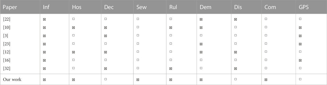
TABLE 1. Features in related works.

Additionally, Pu et al. [32] propose a dynamic adaptive spatio-temporal graph network (DASTGN) based on attention mechanisms, which they test on three COVID-19 datasets from China, Austria, and Brazil.

In addition to being the first epidemic prediction GNN applied to the Netherlands at the fine-grained municipality scale, we show in Table 1 that we also introduce new dataset features to improve predictions. In the Table, the infections (Inf) category includes various measures of infection status, such as the number of reported infections, active infections, incidence rate or recovered infections. Other categories include hospitalizations (Hos), deceased patients (Dec), virus loads in sewage water (Sew), and features related to the strictness of the COVID-19 rules (Rul). Demographic (Dem) features such as the population size and density are also included. Finally, either the distance (Dis) between municipalities, commuting information (Com), or GPS-based mobility data (GPS) are used to connect regions. In this work, we are the first to incorporate virus loads in sewage water and commuter information into our analysis. Additionally, our approach to incorporating the strictness of COVID-19 rules more accurately reflects real-world conditions. Further details about feature selection can be found in Section 3.1. Furthermore, our study distinguishes itself by the fact that we have collected data over a period of almost 2 years, allowing us to compare the results of different COVID-19 variants.

In Table 2, we compare the temporal and spatial layers of the models used in previous works with our own approach. All the spatio-temporal GNN methods discussed consist of temporal layers that model the evolution of the epidemic over time and spatial layers that capture the interactions between different locations. In addition to these core components, these models may also incorporate additional deep learning components such as fully connected layers, dropout layers, and skip connections to improve performance. Our approach is the first to use GATv2 [33] as a spatial component, and we propose a unique and optimized combination of deep learning components, which will be further described in Section 3.2.

TABLE 2

TABLE 2. Models in related works.

3 Methodology

In this section, we present the methods used for developing the COVID-19 dataset and predicting the course of the disease. More specifically, Section 3.1 presents the constructed graph, Section 3.2 reviews the proposed model architecture, Section 3.3 clarifies how we optimize this model, and Section 3.4 describes how the optimized model is used for making predictions.

3.1 Graph construction

In order to make municipality-level predictions for the Netherlands using GNNs, we developed a graph-structured dataset containing information on COVID-19 statistics, demographics, and information on interregional interactions. The resulting undirected graph $\text{G}(\mathcal{V},\mathcal{E})$ represents the model’s input data and consists of a set of nodes $\mathcal{V}$ with node features, and a set of edges $\mathcal{E}$ with associated weights. In addition, we use the graph’s node labels as a ground truth for supervised learning.

Graph nodes In the graph G, all 344 Dutch municipalities are modeled as an individual node. Here, $n=|\mathcal{V}|$ denotes the number of nodes. The graph is visualized in Figure 1.

FIGURE 1

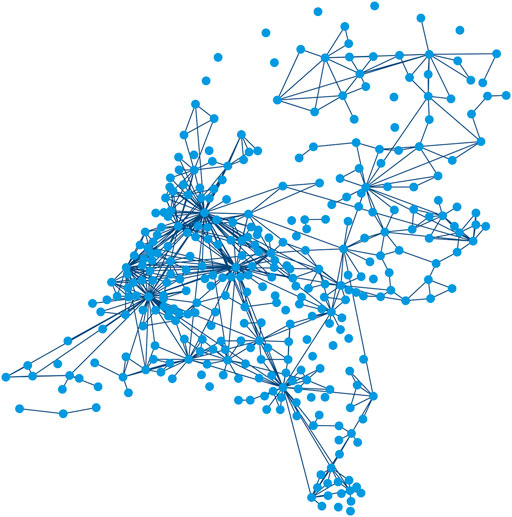
FIGURE 1. Input graph G consisting of a set of nodes $\mathcal{V}$ corresponding to the municipalities of the Netherlands and a set of edges $\mathcal{E}$ representing the connections between them.

Graph edges and weights We construct the edges of the graph based on the assumption that mobility rates between pairs of municipalities influence each other’s infection rates [5]. We use a proxy to quantify mobility, as travel data of people between municipalities is not available for privacy reasons. To determine the most effective proxy for our application, we constructed and evaluated various graphs with different edge configurations and weights. Besides a randomly chosen graph configuration, the edge locations and weights we tested are based on distance between municipalities, distance in combination with population sizes [37], a fitted gravity model [38], and commuter information [39]. We adopted the last graph configuration for the remainder of this research, since this was found to be the most effective. The data about the place of residence and work of employees is collected by Statistics Netherlands (CBS). In our graph, edges connect municipality pairs with at least 1,000 daily commuters. Please note that, limited by the available data, we assume that this measure of mobility remains constant over time. Furthermore, we presume that travelling individuals visit only one region and return to their home region directly afterward.

As a result, we obtain the adjacency matrix $\mathbf{A}\in {\mathbb{R}}^{n\times n}$. This matrix indicates which municipalities are connected and how strong these connections are, and is defined as

${\mathbf{A}}_{ij}=\left\{\begin{array}{cc}{w}_{ij}\hfill & \text{\hspace{0.17em}if\hspace{0.17em}}{e}_{ij}\in \mathcal{E}\text{\hspace{0.17em}and\hspace{0.17em}}i\ne j\hfill \\ 0\hfill & \text{\hspace{0.17em}otherwise,\hspace{0.17em}}\hfill \end{array}\right.(1)$

where w_ij is the normalized weight for each two regions i and j with an existent edge e_ij between them.

Node features Each node or municipality of the graph has a set of associated features $\mathcal{F}$ to provide additional information useful for making more accurate predictions. The node features we include in our developed dataset are.

• Incidence: the daily number of reported COVID-19 cases per unit of population [40, 41].

• Hospitalizations: the daily number of COVID-19 hospital admissions [40].

• Virus load in sewage water: the average concentration of SARS-CoV-2 RNA, converted to the daily amount of sewage water (flow rate) and displayed per 100,000 inhabitants [40].

• Stringency Index: a country-wide composite measure indicating the strictness of the applicable COVID-19 control measures, based on nine response indicators including school closures, workplace closures, and travel bans [42, 43].

• Population density: the number of inhabitants per square kilometer of land area [44].

The feature selection process started with an initial set of ten features, which was based on data and expertise available within the RIVM. Five features were not included in the dataset due to their relatively lower correlation with the ground truth or their negative impact on the model’s performance. These features include the population size, daily number of reported infections and deaths, vaccination rate, and day of the week.

Each feature is normalized to ensure that all features are on the same scale, ranging from 0 to 1. Except for the static population density, we assume that the above-mentioned node attributes are dynamic and change on a daily basis. Subsequently, it is important to note that at each time step t (in days) the features are represented as vectors that stretch back d days, including day t. This means that the values in this feature vector correspond to days t+1-d to t. Together, these feature vectors are presented in a time dependent feature matrix ${\mathbf{X}}^t\in {\mathbb{R}}^{n\times d\times f}$, where n denotes the number of municipalities and $f=|\mathcal{F}|$ the number of features.

Node labels The graph has a time-varying associated node label per municipality, which is equal to the ground truth. While the goal of this paper is to forecast the number of reported SARS-Cov-2 infections 7 days ahead, we train the model on the normalized incidence of this day instead. The reason for training on incidence is the disproportionate distribution of municipalities’ population sizes, and hence also of their infection numbers. By optimizing on incidence instead of infections, we compensate for the population size and prevent the model from focusing too much on the forecasts for the largest municipalities of the Netherlands. Training on incidence means that our node label vector ${\mathbf{y}}^{t+7}\in {\mathbb{R}}^n$ on prediction day t+7 is calculated as

${\mathbf{y}}^{t+7}=\text{normalize}\left(\frac{{\mathbf{I}}^{t+7}}{\mathbf{p}}\right),(2)$

where ${\mathbf{I}}^{t+7}\in {\mathbb{R}}^n$ represents the daily number of reported infections per municipality on day t+7 and $\mathbf{p}\in {\mathbb{R}}^n$ denotes the region’s population sizes [40, 41].

When evaluating the performance of our trained model, we use the data on the observed daily number of reported infections per municipality I^t+7 directly. For real-world application, it is particularly important that epidemic forecasting models can properly predict the trend of infection rates within municipalities. Initiating local measures or allocating resources will in practice not occur daily, which allows policymakers to act on a prediction of the infection trend. Therefore, we also evaluate the model’s performance relative to the trend of the observed infection numbers ${\mathbf{I}}_{\text{trend}}^{t+7}\in {\mathbb{R}}^n$ instead of these numbers themselves. As a trend, we define the moving average of the observed infection numbers.

3.2 The model

Since we would like to capture COVID-19 spread both over time and between municipalities, we propose a spatio-temporal GNN model. Because recurrent neural networks provide a way to extend deep learning to sequential data, we first apply deep learning layers of this type to find temporal patterns in the changing node features of municipalities. Gated recurrent units (GRUs) and long short-term memories (LSTMs) are the most effective sequence models used in practical applications, due to their ability to effectively and accurately retain long-term dependencies in sequential data [45–47]. Based on the observation that the GRU outperforms the LSTM for our application, we decided to include this technique in our model.

After applying the GRU and obtaining the resulting node embedding ${\mathbf{h}}_{\text{GRU}}^t$, we employ a GNN to model the spatial disease transmission patterns caused by the relationship between municipalities. Essentially, the GNN updates each municipality’s node embedding by aggregating the information municipalities receive from their adjacent neighbors. Nowadays, graph attention networks (GATs) as proposed by Veličković et al. [36] are one of the most popular and widespread GNN architectures [48]. Additionally, Brody et al. [33] have proposed the closely related GATv2 recently, which outperforms GAT on all their benchmarks. Based on these results and the performance evaluation on our developed dataset, we decided to use GATv2 to capture the spatial trends in disease transmission. We modify the GATv2 model with skip-connections between layers to avoid diluting the self-node embeddings. Specifically, we concatenate the output of each GATv2 layer with the learned temporal embedding, before we apply the ReLU activation function.

Finally, we need to map the output of the final GATv2 layer ${\mathbf{h}}_{\text{GAT}}^t$ to the desired output dimension, for which we use a fully connected (FC) linear output layer.

We visualize our proposed model in Figure 2, and describe each of its elements in more detail below. Please note that we optimized the number of layers of the architecture based on performance, resulting in a model consisting of two GRU modules, two GATv2 modules, and one fully connected output layer.

FIGURE 2

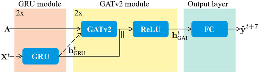
FIGURE 2. The proposed architecture is made up of three stages, being the GRU module in orange, the GATv2 module in yellow, and the output layer in green. Both the GRU module and the GATv2 module are repeated once. Therefore, the dashed input arrows X^t and ${\mathbf{h}}_{\text{GRU}}^t$ imply that for the second layer of their corresponding module, they are replaced by the output embeddings of the module’s first layer.

3.2.1 Gated recurrent unit (GRU) module

The two layer GRU module uses the node feature matrix ${\mathbf{X}}^t\in {\mathbb{R}}^{n\times d\times f}$ as an input. The goal is to retrieve an output embedding ${\mathbf{h}}_{\text{GRU}}^t\in {\mathbb{R}}^{n\times \text{GRU}-\text{dim}}$, which captures the temporal patterns of the dynamic node features over a window of the past d days for each node. This new representation for the municipalities corresponds to the hidden state of the last time step t of the second GRU layer, and is calculated as follows:

${\mathbf{h}}_{\text{GRU}}^t=\text{GRU}\left(\text{GRU}\left({\mathbf{X}}^t,{\mathbf{h}}_0\right),{\mathbf{h}}_0\right),(3)$

where ${\mathbf{h}}_0\in {\mathbb{R}}^{n\times \text{GRU}-\text{dim}}$ is a matrix filled with zeros, corresponding to the initial hidden state before the first day of the time window.

3.2.2 Graph attention network v2 (GATv2) module

In the GATv2 module, the temporal node embedding ${\mathbf{h}}_{\text{GRU}}^t$ is updated per municipality by the GATv2 mechanism [33] using the update rule

${\mathbf{h}}_i^{\prime }={\displaystyle \sum _{j\in \mathcal{N}\left(i\right)}}{\alpha }_{ij}\mathbf{W}{\mathbf{h}}_j,(4)$

where ${\mathbf{h}}_i^{\prime }$ is the updated embedding of node i, and h_j is the node representation of node j of the previous layer, initially being ${\mathbf{h}}_{\text{GRU},j}^t$. We use the graph structure as represented by the weighted adjacency matrix $\mathbf{A}\in {\mathbb{R}}^{n\times n}$ by exclusively summing over the nodes j that are part of the set of neighbors of node i, $\mathcal{N}(i)$, in a weighted manner. We consider node i itself to be part of this neighborhood as well. Furthermore, W is a learnable weight matrix associated with each node’s linear transformation and α_ij is the normalized attention coefficient. This value quantifies the connective strength between the node i and its neighbor j using an attention mechanism

${\alpha }_{ij}=\frac{\exp \left({\mathbf{a}}^{\top }\mathrm{L}\mathrm{e}\mathrm{a}\mathrm{k}\mathrm{y}\mathrm{R}\mathrm{e}\mathrm{L}\mathrm{U}\left(\mathbf{W}\left[{\mathbf{h}}_i\Vert {\mathbf{h}}_j\right]\right)\right)}{{\sum }_{k\in \mathcal{N}\left(i\right)}\exp \left({\mathbf{a}}^{\top }\mathrm{L}\mathrm{e}\mathrm{a}\mathrm{k}\mathrm{y}\mathrm{R}\mathrm{e}\mathrm{L}\mathrm{U}\left(\mathbf{W}\left[{\mathbf{h}}_i\Vert {\mathbf{h}}_k\right]\right)\right)},(5)$

where a^T is a transposed vector of learnable parameters, and ‖ is the concatenation operation.

To stabilize the self-attention learning process and to improve its expressive power, the GATv2 model uses multi-head attention [33, 36]. This implies that K independent attention mechanisms perform the transformation described above, and subsequently concatenate their outputs to create the final node representation.

The two layered GATv2 module and its resulting spatio-temporal embedding ${\mathbf{h}}_{\text{GAT}}^t\in {\mathbb{R}}^{n\times \text{GAT}-\text{dim}}$ can thus be represented as

$\begin{array}{cc}\hfill {\mathbf{h}}^t& =\text{ReLU}\left(\text{GATv}2\left({\mathbf{h}}_{\text{GRU}}^t,\mathbf{A}\right)\Vert {\mathbf{h}}_{\text{GRU}}^t\right)\hfill \\ \hfill {\mathbf{h}}_{\text{GAT}}^t& =\text{ReLU}\left(\text{GATv}2\left({\mathbf{h}}^t,\mathbf{A}\right)\Vert {\mathbf{h}}_{\text{GRU}}^t\right).\hfill \end{array}(6)$

3.2.3 Output layer

Finally, we need to map the output of the final hidden layer to the desired output dimension. Therefore, we feed the hidden state obtained by the GATv2 module ${\mathbf{h}}_{\text{GAT}}^t$ to a fully connected (FC) linear output layer

${\widehat{\mathbf{y}}}^{t+7}=\text{FC}\left({\mathbf{h}}_{\text{GAT}}^t\right).(7)$

As a result, we predict the normalized incidence vector ${\widehat{\mathbf{y}}}^{t+7}\in {\mathbb{R}}^n$ containing predictions for each municipality 7 days ahead.

3.3 Optimization

We propose to optimize the model for 7 day ahead prediction directly [22], following the pseudocode described in Algorithm 1. We use the mean squared error (MSE) as our loss function

$\mathcal{L}=\frac{1}{nT}{\displaystyle \sum _{t=1}^T}{\displaystyle \sum _{i=1}^n}{\left(y_i^{t+7}-{\widehat{y}}_i^{t+7}\right)}^2,(8)$

since it is commonly used in regression tasks and encourages the model to minimize large errors [49]. Here, n denotes the number of municipalities and T the number of days on which we train the model. Furthermore, $y_i^{t+7}$ refers to the reported infection incidence for municipality i at day t+7 and ${\widehat{y}}_i^{t+7}$ to the associated predicted infection incidence as obtained by the model.

Algorithm 1.: Training the model.

• Input: Time series node feature and node label data {X, y}, adjacency matrix A, learning rate η

• Output: Model parameters Θ Initialize Θ randomly

•  for each epoch do

•   for each timestep t do

•    ${\mathbf{h}}_{\text{GRU}}^t=\text{GRU\hspace{0.17em}module}({\mathbf{X}}^t)$

•    ${\mathbf{h}}_{\text{GAT}}^t=\text{GATv}2\text{\hspace{0.17em}module}({\mathbf{h}}_{\text{GRU}}^t,\mathbf{A})$

•    ${\widehat{\mathbf{y}}}^{t+7}=\text{Output\hspace{0.17em}layer}({\mathbf{h}}_{\text{GAT}}^t)$

•    $\text{error}+=\text{MSE}({\mathbf{y}}^{t+7},{\widehat{\mathbf{y}}}^{t+7})$

•   end for

•   $\mathcal{L}(\mathbf{\Theta })=\frac{1}{T}\text{error}$

•   $\mathrm{\Delta }\mathcal{L}(\mathbf{\Theta })=\text{BackProp}(\mathcal{L}(\mathbf{\Theta }),\mathbf{\Theta })$

•   $\mathbf{\Theta }=\mathbf{\Theta }-\eta \mathrm{\Delta }\mathcal{L}(\mathbf{\Theta })$

•  end for

•  return Θ

3.4 Prediction

We apply the trained model to predict the number of reported COVID-19 cases ${\widehat{\mathbf{I}}}^{t+7}\in {\mathbb{R}}^n$ in all municipalities on day t+7 using the equation

${\widehat{\mathbf{I}}}^{t+7}=\mathbf{p}*\text{denormalize}\left({\widehat{\mathbf{y}}}^{t+7}\right).(9)$

Here, $\mathbf{p}\in {\mathbb{R}}^n$ is the population size per municipality and ${\widehat{\mathbf{y}}}^{t+7}\in {\mathbb{R}}^n$ the predicted incidence, which is converted back to its original scale.

4 Experiments

This section introduces the datasets we used in Section 4.1, refers to our comparison methods in Section 4.2, describes the evaluation metrics used in Section 4.3, and explains the hyperparameters and implementation details in Section 4.4.

4.1 The dataset

We use open data from three sources: the COVID-19 dataset of the National Institute for Public Health and the Environment (RIVM) [40], data from Statistics Netherlands (CBS) [39, 41, 44], and the Oxford COVID-19 Government Response Tracker [42, 43]. We fuse these datasets to obtain the necessary graph edge, node feature, and node label information.

While the first COVID-19 case in the Netherlands was discovered on 27 February 2020, our study period is from 1 June 2020, until 10 April 2022. In the Netherlands, testing capacity was limited before 1 June 2022, so the number of positive tests did not reflect the actual number of SARS-Cov-2 infections. The same applies to all days after 10 April 2022, because from then on, the advice to confirm a positive self-test at the Dutch Municipal Health Service was canceled, except for specific target groups such as healthcare workers [50, 51].

To ensure real-world application of our method, we chose to divide the study period into shorter time intervals of 61 days. By training on the first 53 and validating on the subsequent 7 days of each interval, we guarantee that our model can be used for prediction on test day 61. Because there have been only four widespread COVID-19 variants (i.e., the wild type, alpha, delta, omicron) [52], it is difficult for the model to capture the differences between them. Therefore, we make sure that in each time period at least 75% of all test samples of SARS-Cov-2 infected persons that are sequenced by the pathogen surveillance consist of the same variant [53].

Although users would in real life retrain the model every day to make a prediction based on the most recent data, we chose to predict for 14 days in this paper. This allows us to balance the need for computational efficiency with the ability to examine differences in performance over time and between variants. We present the associated 14 time periods and their characteristics in Table 3.

TABLE 3

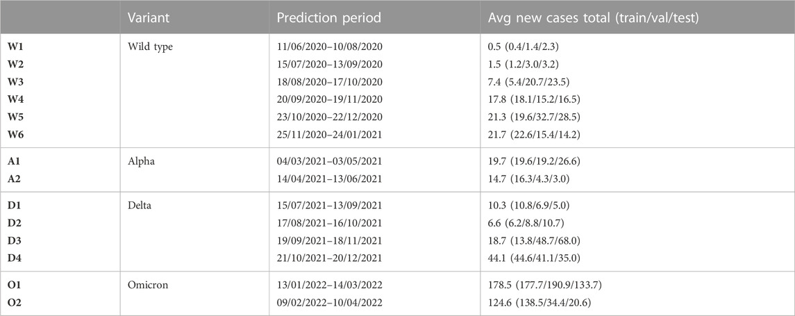
TABLE 3. Time period characteristics.

In Figure 3, we visualize the split in training, validation, and test data by means of a plot of the aggregated number of infections in the Netherlands over period D3, corresponding to a time when the delta variant was dominant, and the infection numbers were increasing. Once the model is trained, day t is the day up until which data is used to make t+7 predictions for the test day on 18 November 2021. In Appendix A, these plots are presented for the other periods as well.

FIGURE 3

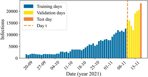
FIGURE 3. The aggregated number of reported COVID-19 cases in the Netherlands over the prediction days of time period D3, with the days included in the training set in blue, the validation set in yellow, and the test set in orange. Once the model is trained, we use data up to and including day t (dashed orange line) to predict infections on the test day at t+7.

4.2 Comparison methods

Our approach involves applying the proposed method on the newly developed COVID-19 dataset, which is why no baselines yet exist to compare our model to. Therefore, we implemented various simple and commonly used baselines [3, 16]. According to these baselines, the prediction for day t+7 is equal to.

1) PD: the number of reported cases on day t.

2) HA: the historical average of the number of reported cases up to and including day t.

3) HA_window: the historical average of the number of reported cases in observation window d (day t+1-d to day t).

4) EB: the number of reported cases on day t multiplied with $\lambda \left({\widehat{\mathbf{y}}}^{t+7}=\lambda {\mathbf{y}}^t\right)$, where λ is determined based on the infection rates of observation window d.

In order to gain a better understanding of the proposed spatio-temporal GNN’s behavior, we perform an ablation study. We investigate the influence of the GRU and GATv2 modules on the performance of the developed model by removing them one at a time, resulting in the following architectures.

1) GRU: A temporal model consisting of the GRU module and the output layer.

2) GATv2: A spatial model consisting of the GATv2 module and the output layer.

4.3 Evaluation metrics

To quantify the difficulty of making predictions for the developed dataset, we propose the fluctuation size per municipality as a metric that measures the fluctuations in the data. The fluctuation size Fl_i of municipality i is calculated as follows:

$F{l}_i=\frac{1}{T-1}{\displaystyle \sum _{t=1}^{T-1}}|{\tilde{I}}_i^{t+1}-{\tilde{I}}_i^t|,(10)$

where T is equal to the number of time steps in the considered time period, and ${\tilde{I}}_i^{t+1}$ and ${\tilde{I}}_i^t$ are the normalized observed number of reported infections in the municipality i at times t+1 and t.

The objective of this study is to predict the number of SARS-Cov-2 infections as accurately as possible, which is defined by the error between the observed infections ${\mathbf{I}}^{t+7}\in {\mathbb{R}}^n$ and predicted infections ${\widehat{\mathbf{I}}}^{t+7}\in {\mathbb{R}}^n$. Lower errors indicate higher prediction accuracy. We especially aim to minimize relatively large errors, as these can result in inaccurate control measures and resource allocation. Therefore, we adopt the root mean squared error (RMSE) [54] over all municipalities on each test day as an evaluation metric.

Besides the RMSE, we also introduce a scale independent metric, the coefficient of determination (R²) [54]. This metric assesses the correlation between observed and predicted number of infections. A R² close to one suggests a perfectly accurate prediction, while a R² close to or below zero indicates that the model fails to make accurate predictions. Please note that we also use the RMSE and R² metrics when evaluating the performance of the model relative to the trend of the observed infection numbers ${\mathbf{I}}_{\text{trend}}^{t+7}\in {\mathbb{R}}^n$.

When evaluating the forecast of the model for an individual municipality on a specified day, we would like to use an evaluation metric that is easy to interpret. Therefore, we use the absolute error between the municipality’s observed number of infections and the predicted number of infections.

4.4 Hyperparameter setting and implementation details

In Table 4, we present the hyperparameters that have been used for the final model. The mentioned hidden dimensions correspond to the two GRU layers and the two GATv2 modules, and the number of independent attention heads K to the two GATv2 layers. With early stopping, we store the parameters of the model that achieved the highest validation accuracy, and then retrieve it to make predictions about the test samples. The model is implemented with Porch [55] and Porch Geometric [56]. For all our experiments, we use a look-back window d of 7 days, and the aforementioned prediction horizon h of 7 days.

TABLE 4

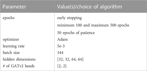
TABLE 4. Hyperparameters.

5 Results

In this section, we present the obtained results, where Section 5.1 focuses on the dataset and Section 5.2 on the model.

5.1 The dataset

To evaluate the proposed approach on the developed COVID-19 dataset, we first determine the difficulty of making predictions for the developed dataset by calculating the fluctuation sizes Fl for our time periods. Taking time period D3 as an example, we see that during this period of time the fluctuation size for the Netherlands as a whole is equal to 0.031, while the average over the individual municipalities is equal to 0.098, meaning that the fluctuation of individual municipalities is on average 3.2 times as large as of the Netherlands. Averaged over all time periods, the mean fluctuation size of individual municipalities is 2.3 times as large as of the Netherlands as a whole.

We present a visualization of the normalized actual number of reported infections and its fluctuations during time period D3 for the whole of the Netherlands and for two example municipalities, Oost Gelre and Rotterdam, in Figure 4. Here, the fluctuations in Oost Gelre are 3.8 times as large, and for Rotterdam 2.5 times as large as in the Netherlands.

FIGURE 4

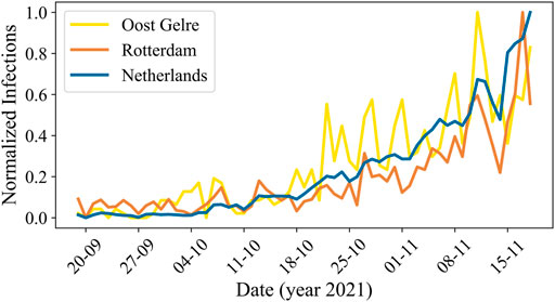
FIGURE 4. The normalized actual number of reported COVID-19 cases over time in the Netherlands for period D3. The blue line corresponds to the total number of infections in the Netherlands, the yellow line to the municipality Oost Gelre, and the orange line to the municipality Rotterdam.

5.2 The model

In Table 5 and Table 6, we report the RMSE and the R² performance metrics for the prediction of our spatio-temporal GNN model, its GRU and GATv2 components, and the baselines for the different time periods of our dataset. Here, the numbers in bold indicate which of these concepts perform best on the test day of each time period, and underlined numbers present the corresponding best baseline. It is notable that both the performance of our proposed model and the baselines vary widely across the different time periods. The proposed model’s minimum coefficient of determination is 0.004 for the first omicron period O1, which indicates that the model fails to make accurate predictions during this time period. Meanwhile, the R² of 0.934 for the last delta time period D4 suggests that the model explains as much as 93.4% of the variance of our forecasts.

TABLE 5

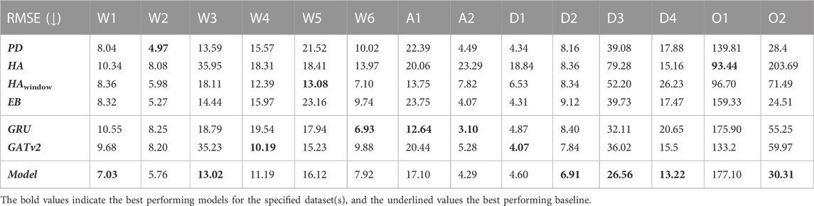
TABLE 5. The root mean squared errors (RMSE) of the developed model, the GRU and GATv2 components, and the baselines for all 14 time periods. Numbers in bold indicate the lowest RMSE per time period, underlined numbers present the corresponding best performing baseline.

TABLE 6

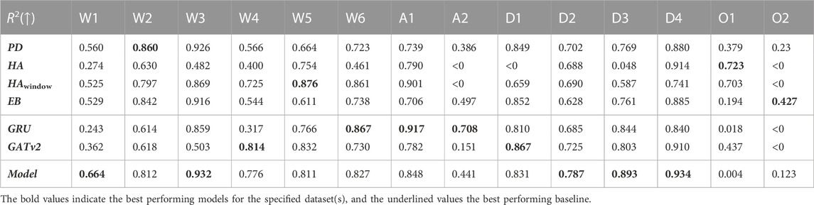
TABLE 6. The coefficients of determination of the developed model, the GRU and GATv2 components, and the baselines for all 14 time periods. Numbers in bold indicate the highest R² per time period, underlined numbers present the corresponding best performing baseline.

In Table 7 and Table 8, we report the average performances over all 14 time periods (Avg), and over the four COVID-19 variants being the wild type (WT), alpha α), delta δ), and omicron o). It is not fair to compare the RMSE over the time periods, because the interpretation of a given RMSE is highly dependent on the predicted number of infections. For example, a RMSE of 10 infections while there are 200 infections predicted is not important for policymaking and resource relocation, as opposed to a RMSE of 10 infections with a prediction of 20 infections. Therefore, we only report the RMSE relative to the baselines and its parts in Table 7. Here, we notice that averaged over all time periods, the RMSE of our model is −9.8% relative to the best performing baseline PD, meaning that on average our proposed model achieves a 9.8% lower RMSE than this baseline. Looking at Table 8, we find that the average coefficient of determination of the proposed model 0.696, which is 3.2% higher than of the best performing baseline PD. These results show that on average, our model can conduct more accurate predictions than the baselines, and that the relationship between the actual values and our model’s predictions accounts for 69.6% of the variation in the predictions.

TABLE 7

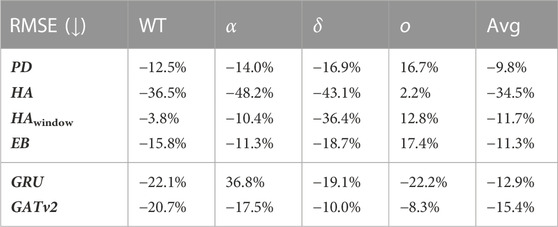
TABLE 7. The average relative RMSE prediction performance of our model with respect to its parts and the baselines for each COVID-19 variant and in total.

TABLE 8

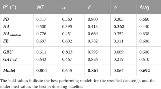
TABLE 8. The average coefficient of determination of our model, its parts, and the baselines for each COVID-19 variant and in total. Numbers in bold indicate the highest R² per variant, underlined numbers present the corresponding best performing baseline.

By looking at the performance of the model per COVID-19 variant in Table 7 and Table 8, we notice that our proposed model achieves a lower RMSE and a higher R² than all the baselines for the wild type, alpha, and delta variant. Looking at the coefficient of determination, we see that relative to the PD baseline, this value increases with 8.7% for the wild type, 8.2% for the alpha variant, and 6.1% for the delta variant. For these variants, we note that the average coefficient of determination is 0.795. Meanwhile, we notice that the performance of the proposed model is worse than all baselines for the omicron variant.

5.2.1 The GRU and GATv2 modules

Table 5 and Table 6 also contain the RMSE and R² evaluation metrics for the exclusively temporal GRU model and the solely spatial GATv2 model. As with our proposed model and the baselines, there is a large variation between the time periods. While the R² of the GRU and the GATv2 are both below zero for the second omicron period O2, the GRU achieves a R² of 0.917 for period A1 and the GATv2 a R² of 0.910 for period D4.

Table 7 and Table 8 show that on average the RMSE of our spatio-temporal model is 12.9% lower, and the coefficient of determination 8.6% higher than of the temporal GRU model. Similarly, the model’s RMSE is 15.4% lower than the GATv2 model, and the corresponding R² score is 8.2% higher. For our application, the performance of the proposed spatio-temporal GNN is thus higher than of the temporal GRU model or the spatial GATv2.

5.2.2 Individual municipalities

To further evaluate the performance of our model on the developed COVID-19 dataset, we also look at our forecasts for individual municipalities. Hence, we visualize the correlation between the observed and the predicted number of reported SARS-Cov-2 infections of period D3 in Figure 5, which we present for the other time periods in Appendix B. The blue dots indicate the 18 November 2021, forecasts for all 344 municipalities.

FIGURE 5

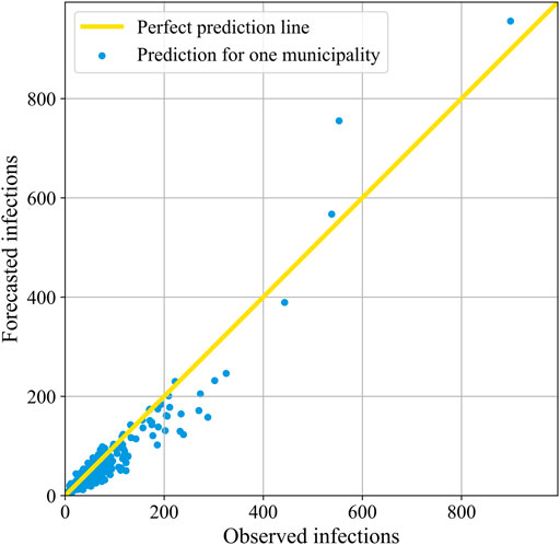
FIGURE 5. The correlation between the forecasted and the observed number of reported COVID-19 cases in period D3. Here, each blue dot corresponds to the forecast for one municipality 18 November 2021. When a dot lies on the yellow diagonal line, it means that the prediction is perfect.

It is apparent from the plot that there is a high number of municipalities with low infection rates. Accordingly, there are more small municipalities than large ones in the Netherlands. The dots of most of the municipalities are quite close to the 45° yellow line through the origin, which corresponds to the high coefficient of determination of 0.893 that we presented for period D3 in Table 6. In general, the model thus appears to be both accurate and precise. However, for the municipalities with less than 400 infections, the mean of the dots is in an increasing manner slightly below the perfect prediction line, indicating that the accuracy is not perfect and that the model increasingly underestimates the number of infections. There are only four municipalities with more than 400 observed infections, being the four biggest municipalities of the Netherlands; Amsterdam, Rotterdam, ‘s-Gravenhage, and Utrecht. In contrast to the smaller municipalities, their predictions are on average above the actual infections.

As an illustration of the variation between municipalities, Table 9 and Table 10 present the absolute difference between the predicted and the actual number of infections for individual municipalities on 18 November 2021. Here, Table 9 shows the three municipalities with the smallest error, being Oost Gelre, Meierijstad, and Opsterland, and Table 10 the three worst performing municipalities, being Rotterdam, Maastricht, and Heerlen. As we have seen before with the variation between the time periods, it appears here that the variation on the same day between municipalities is also large, with a minimum error of approximately zero infections in Oost Gelre, Meierijstad, and Opsterland, and a maximum error of 202 infections in Rotterdam. Relatively speaking, the differences are also large. Indeed, the error relative to the number of infections is below 1% for Oost Gelre, Meierijstad and Opsterland, while it is 36.6% for Rotterdam, 45.2% for Maastricht and 48.5% for Heerlen.

TABLE 9

TABLE 9. The absolute error for the proposed model and its baselines for the best performing municipalities for prediction on 18/11/2021 (period D3).

TABLE 10

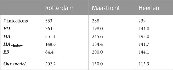
TABLE 10. The absolute error for the proposed model and its baselines for the worst performing municipalities for prediction on 18/11/2021 (period D3).

We present plots corresponding to the predictions of these municipalities in Figure 6. Please note that, next to our proposed model and the actual values, we chose to visualize only the best performing baseline in each prediction for clarity. It is noticeable here that the data contains a lot of noise due to the rapid fluctuations. Therefore, it seems that while our model often captures the right trend, it is unable to interpret these rapid changes.

FIGURE 6

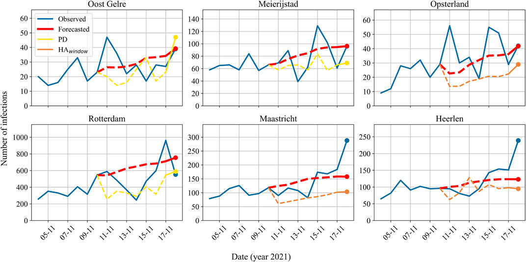
FIGURE 6. The actual and predicted reported number of infections for individual municipalities on 11/18/2021 (period D3). Based on the absolute difference between the prediction and the actual value, the upper row corresponds to the best performing municipalities (Oost Gelre, Meierijstad, Opsterland) and the bottom row to the worst performing municipalities (Rotterdam, Maastricht, and Heerlen). The blue line indicates the actual number of infections reported, the red line the model’s predictions, and either the yellow or the orange line the predictions of the baselines. Note that for clarity of illustration, the plots only visualize the best performing baseline in each prediction. In the plots, the dashed lines represent predictions in the validation set, and the dots represent the prediction on test day 18/11/2021.

5.2.3 The trend

As explained in before, we would also like to analyze the performance of our proposed model for infection trend prediction. We present an example of the actual infection curve and the trend for Rotterdam on 18 November 2021, in Figure 7.

FIGURE 7

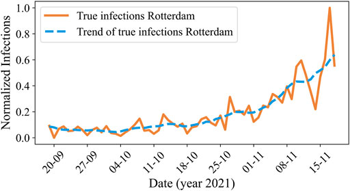
FIGURE 7. The normalized actual number of reported COVID-19 cases (orange) and its trend (blue) over time in Rotterdam for period D3.

If we evaluate our model against the trend rather than actual infection values, the performance improves significantly. Where the average coefficient of determination for actual infection prediction is 0.692, it increases to 0.851 for prediction of the trend, indicating a 15.9% gain. For each variant specifically, the coefficients of determination for trend prediction are 0.898 for the wild type, 0.831 for alpha, 0.934 for delta, and 0.562 for omicron. We give an overview of the improvements of the trend predictions compared to the actual value predictions of our model in Table 11. It is evident that, across all variants and on average, our model exhibits superior performance in predicting the trend of infection rates compared to the highly variable actual rates.

TABLE 11

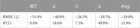
TABLE 11. The performance of the proposed model for trend predictions compared to actual value predictions.

5.2.4 The forecasting horizon

We would like to understand if our varying performance is caused by the prediction horizon h of 7 days, or whether the cause is in our dataset or model itself. Therefore, we also made t+1 forecasts for the exact same days as with the t+7 forecasts. For these t+1 forecasts, the coefficients of determination are 0.845 on average, 0.863 for the wild type, 0.750 for alpha, 0.882 for delta, and 0.845 for omicron. We present the relative performances of our 7-day multistep prediction with respect to the performance of the model when predicting only 1 day ahead in Table 12. Comprehensive results of the 1-day ahead forecast can be found in Appendix C.

TABLE 12

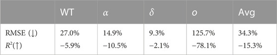
TABLE 12. The relative prediction performance for T+7 with respect to T+1.

As presented earlier in literature [12, 16, 22], we share the observation that for both the individual COVID-19 variants and the average, the performance of the model decreases as the prediction horizon increases. On average, the RMSE increases with 34.3%, and the coefficient of determination decreases with 15.3%. By looking at the individual variants, we particularly notice that the results of our model for the omicron variant deteriorate relatively much, with a RMSE increase of 125.7% and a coefficient of determination decrease of 78.1%.

6 Discussion

The variation in results as demonstrated in Section 5.2, can be explained by the observation that the daily numbers of reported SARS-Cov-2 infections per municipality have a high fluctuation size. We also note that there are significant differences in the data between the chosen time periods and between municipalities, such as the order of magnitude of the infection rates and the dynamic node features (e.g., the virus load in sewage water), and the shape of the infection curve. Between time periods, the variants circulating vary as well. Additionally, there are variations between municipalities in population size, population density, and the number of neighbors. These aspects of the dataset make it challenging to capture the resulting complex relationships, and to obtain accurate predictions for all time period and municipality combinations.

Despite these challenges, the average performance of our model in predicting the spread of SARS-CoV-2 at the municipal level in the Netherlands is strong. We observed that the performance of the proposed spatio-temporal GNN outperforms its temporal and spatial components, proving the effectiveness of modelling the spreading of epidemic diseases as a spatio-temporal problem. Nevertheless, we hypothesize that if related data would be available, the performance of the spatial GATv2 module could be enhanced through the use of a more representative strategy for selecting edge locations and weights.

As discussed in Section 5.2, both our model and the baselines struggle to make accurate predictions for the omicron variant. This suggests that omicron is a particularly challenging variant to predict. This may be due to the fact that omicron is more contagious and produces milder symptoms compared to earlier variants, leading to more rapid changes in the number of cases [57]. Another potential explanation could be the occurrence of natural immunity in individuals due to the high number of infections during the omicron period [40], leading to a decrease in transmission during this period as a result of the increased protection.

In order to improve the overall prediction performance (including that of the omicron variant), a model capable of capturing more complex relationships would be required. To obtain such models, we either increased the number of GRU layers, the number of GATv2 layers, or the hidden dimension sizes. Evaluation of these models demonstrated that utilizing these adapted models with the limited available data a decrease in performance. To effectively utilize a more complex model, an increased amount of data, such as synthetic data or data from other countries, would be necessary.

In future work, it may also be worth considering a larger regional scale, such as the 25 security regions of the Netherlands instead of the 344 municipalities. This approach could potentially decrease the fluctuation size and complexity of relationships, making it easier for the model to capture the relationship of infection numbers over time and between regions, while still allowing for the implementation of regional measures or resource distribution.

7 Conclusion

In this paper, we introduced a novel model architecture for forecasting reported SARS-Cov-2 infections 1 week ahead using a spatio-temporal GNN. We applied our model to a newly introduced COVID-19 dataset containing municipality-level information for the Netherlands, including COVID-19 statistics, demographic features, and municipality interaction data.

Our model demonstrates strong performance in predicting the spread of SARS-Cov-2 at the Dutch municipal level for the wild type, alpha, and delta variants. The model outperforms the baselines and the exclusively spatial and temporal models. Additionally, with an average coefficient of determination of 0.795 and the ability to capture the trend of the disease with a R² score of 0.899, we conclude that the model is well-suited for predicting the spread of these variants in real-world applications, allowing policymakers to anticipate and take necessary action in response to the pandemic. However, for the omicron variant the performance is significantly worse with an average coefficient of determination of 0.064 for infection prediction and 0.562 for trend prediction. Therefore, we recommend using more data for more complex disease dynamics, such as those exhibited by the omicron variant. The model could, for example, be pre-trained on data from other countries than the Netherlands or synthetically generated data. Another option is to decrease the complexity of the problem by expanding the regional forecasting scale. For instance, by predicting for safety regions instead of municipalities in the Netherlands. In real-world applications, we recommend using our proposed model in combination with a mechanistic model in an ensemble approach to enhance long-term predictions and to improve prediction accuracy and robustness. Future work will investigate this possibility and on combining forecasting models with reactive intervention strategies based on control theory [58–61].

Data availability statement

The original contributions presented in the study are included in the article/Supplementary Materials, further inquiries can be directed to the corresponding author.

Author contributions

VC: Data curation, Investigation, Methodology, Project administration, Software, Visualization, Writing–original draft. SI: Data curation, Project administration, Supervision, Writing–review and editing. CD: Conceptualization, Funding acquisition, Investigation, Project administration, Supervision, Writing–review and editing.

Funding

The author(s) declare that no financial support was received for the research, authorship, and/or publication of this article.

Conflict of interest

The authors declare that the research was conducted in the absence of any commercial or financial relationships that could be construed as a potential conflict of interest.

The author(s) declared that they were an editorial board member of Frontiers, at the time of submission. This had no impact on the peer review process and the final decision.

Publisher’s note

All claims expressed in this article are solely those of the authors and do not necessarily represent those of their affiliated organizations, or those of the publisher, the editors and the reviewers. Any product that may be evaluated in this article, or claim that may be made by its manufacturer, is not guaranteed or endorsed by the publisher.

Supplementary material

The Supplementary Material for this article can be found online at: https://www.frontiersin.org/articles/10.3389/fphy.2023.1277052/full#supplementary-material

References

1. World Health Organization. Managing epidemics: key facts about major deadly diseases. Geneva: World Health Organization (2018).

Google Scholar

2. Dong E, Du H, Gardner L. An interactive web-based dashboard to track COVID-19 in real time. Lancet Infect Dis (2020) 20:533–4. doi:10.1016/s1473-3099(20)30120-1

PubMed Abstract | CrossRef Full Text | Google Scholar

3. Kapoor A, Ben X, Liu L, Perozzi B, Barnes M, Blais M, et al. Examining COVID-19 forecasting using spatio-temporal graph neural networks (2020). https://arxiv.org/abs/2007.03113. (Accessed April 07, 2022).

Google Scholar

4. Jhun B. Effective vaccination strategy using graph neural network ansatz (2021). Available at: http://arxiv.org/abs/2111.00920. (Accessed March 14, 2022).

Google Scholar

5. Schoot Uiterkamp M, Gösgens M, Heesterbeek H, Van Der Hofstad R, Litvak N. The role of inter-regional mobility in forecasting SARS-CoV-2 transmission. J R Soc Interf (2022) 19(193):8. doi:10.1098/rsif.2022.0486

CrossRef Full Text | Google Scholar

6. Kermack W, McKendrick A. A contribution to the mathematical theory of epidemics. Proc R Soc Lond Ser A, Containing Pap a Math Phys character (1927) 115(772):700–91. doi:10.1098/rspa.1927.0118

CrossRef Full Text | Google Scholar

7. Keeling MJ, Eames KT. Networks and epidemic models. J R Soc Interf (2005) 2(4):295–307. doi:10.1098/rsif.2005.0051

PubMed Abstract | CrossRef Full Text | Google Scholar

8. Kandula S, Shaman J. Near-term forecasts of influenza-like illness. Epidemics (2019) 27:41–51. doi:10.1016/j.epidem.2019.01.002

PubMed Abstract | CrossRef Full Text | Google Scholar

9. Chimmula VKR, Zhang L. Time series forecasting of COVID-19 transmission in Canada using LSTM networks. Chaos, Solitons and Fractals (2020) 135:109864. doi:10.1016/j.chaos.2020.109864

PubMed Abstract | CrossRef Full Text | Google Scholar

10. La Gatta V, Moscato V, Postiglione M, Sperli G. An epidemiological neural network exploiting dynamic graph structured data applied to the COVID-19 outbreak. IEEE Trans Big Data (2021) 7(1):45–55. doi:10.1109/tbdata.2020.3032755

PubMed Abstract | CrossRef Full Text | Google Scholar

11. Hinch R, Probert WJ, Nurtay A, Kendall M, Wymant C, Hall M, et al. OpenABM-Covid19 - an agent-based model for non-pharmaceutical interventions against COVID-19 including contact tracing. PLoS Comput Biol (2021) 17(7):e1009146. doi:10.1371/journal.pcbi.1009146

PubMed Abstract | CrossRef Full Text | Google Scholar

12. Gao J, Sharma R, Qian C, Glass LM, Spaeder J, Romberg J, et al. STAN: spatio-temporal attention network for pandemic prediction using real-world evidence. J Am Med Inform Assoc (2021) 28(4):733–43. doi:10.1093/jamia/ocaa322

PubMed Abstract | CrossRef Full Text | Google Scholar

13. Adiga A, Dubhashi D, Lewis B, Marathe M, Venkatramanan S, Vullikanti A. Mathematical models for COVID-19 pandemic: a comparative analysis. J Indian Inst Sci (2020) 100(4):793–807. doi:10.1007/s41745-020-00200-6

PubMed Abstract | CrossRef Full Text | Google Scholar

14. Zhang Z, Cui P, Zhu W. Deep learning on graphs: a survey. IEEE Trans Knowledge Data Eng (2022) 34(1):249–70. doi:10.1109/tkde.2020.2981333

CrossRef Full Text | Google Scholar

15. Wu Z, Pan S, Chen F, Long G, Zhang C, Yu PS. A comprehensive survey on graph neural networks. IEEE Trans Neural Networks Learn Syst (2021) 32(1):4–24. doi:10.1109/tnnls.2020.2978386

CrossRef Full Text | Google Scholar

16. Panagopoulos G, Nikolentzos G, Vazirgiannis M. Transfer graph neural networks for pandemic forecasting. Proc AAAI Conf Artif Intelligence (2021) 35(6):4838–45. doi:10.1609/aaai.v35i6.16616

CrossRef Full Text | Google Scholar

17. Zhou J, Cui G, Hu S, Zhang Z, Yang C, Liu Z, et al. Graph neural networks: a review of methods and applications. AI Open (2020) 1:57–81. doi:10.1016/j.aiopen.2021.01.001

CrossRef Full Text | Google Scholar

18. Liu Z, Zhou J. In: R Brachman, F Rossi, and P Stone, editors. San Rafael, California: Morgan and Claypool (2020).Introduction to graph neural networks

Google Scholar

19. Stokes JM, Yang K, Swanson K, Jin W, Cubillos-Ruiz A, Donghia NM, et al. A deep learning approach to antibiotic discovery. Cell (2020) 180:688–702. doi:10.1016/j.cell.2020.01.021

PubMed Abstract | CrossRef Full Text | Google Scholar

20. Derrow-Pinion A, She J, Wong D, Lange O, Hester T, Perez L, et al. ETA prediction with graph neural networks in Google maps. In: Proceedings of the 30th ACM International Conference on Information and Knowledge Management; October 2021; New York, NY (2021). p. 3767–76.

CrossRef Full Text | Google Scholar

21. Ying R, He R, Chen K, Eksombatchai P, Hamilton WL, Leskovec J. Graph convolutional neural networks for web-scale recommender systems. In: Proceedings of the 24th ACM SIGKDD International Conference on Knowledge Discovery and Data Mining; July 2018; New York, NY (2018). p. 974–83.

CrossRef Full Text | Google Scholar

22. Deng S, Wang S, Rangwala H, Wang L, Ning Y. Graph message passing with cross-location attentions for long-term ILI prediction (2019). Available at: http://arxiv.org/abs/1912.10202. (Accessed April 02, 2022).

Google Scholar

23. Murphy C, Laurence E, Allard A. Deep learning of contagion dynamics on complex networks. Nat Commun (2021) 12(1):4720–11. doi:10.1038/s41467-021-24732-2

PubMed Abstract | CrossRef Full Text | Google Scholar

24. Li Z, Luo X, Wang B, Bertozzi AL, Xin J. A study on graph-structured recurrent neural networks and scarification with application to epidemic forecasting. In: World congress on global optimization. Berli, Germany: Springer (2019). p. 730–9. Available at: http://arxiv.org/abs/1902.05113. (Accessed April 01, 2022).

CrossRef Full Text | Google Scholar

25. Mežnar S, Lavrač N, Škrlj B. Prediction of the effects of epidemic spreading with graph neural networks. In: Complex networks and their applications. Berli, Germany: Springer (2020). p. 420–31.

Google Scholar

26. Wang Y, Zeng DD, Zhang Q, Zhao P, Wang X, Wang Q, et al. Adaptively temporal graph convolution model for epidemic prediction of multiple age groups. Fundam Res (2021) 2:311–20. doi:10.1016/j.fmre.2021.07.007

CrossRef Full Text | Google Scholar

27. Tomy A, Razzanelli M, Di Lauro F, Rus D, Della Santina C. Estimating the state of epidemics spreading with graph neural networks (2021). Available at: http://arxiv.org/abs/2105.05060. (Accessed April 09, 2022).

Google Scholar

28. Cutura G, Li B, Swami A, Segarra S. Deep demixing: reconstructing the evolution of epidemics using graph neural networks (2020). Available at: http://arxiv.org/abs/2011.09583. (Accessed March 31, 2022).

Google Scholar

29. Shah C, Dehmamy N, Perra N, Chinazzi M, Barabási A-L, Vespignani A, et al. Finding patient zero: learning contagion source with graph neural networks (2020). Available at: http://arxiv.org/abs/2006.11913. (Accessed March 18, 2022).

Google Scholar

30. Song S, Zong Z, Li Y, Liu X, Yu Y. Reinforced epidemic control: saving both lives and economy (2020). Available at: http://arxiv.org/abs/2008.01257. (Accessed April 15, 2022).

Google Scholar

31. Meirom EA, Maron H, Mannor S, Chechik G. How to stop epidemics: controlling graph dynamics with reinforcement learning and graph neural networks (2020). Available at: http://arxiv.org/abs/2010.05313. (Accessed April 05, 2022).

Google Scholar

32. Pu X, Zhu J, Wu Y, Leng C, Bo Z, Wang H. Dynamic adaptive spatio–temporal graph network for Covid-19 forecasting. Liangjiang: CAAI Transactions on Intelligence Technology (2023).

Google Scholar

33. Brody S, Alon U, Yahav E. How attentive are graph attention networks? (2021). Available at: http://arxiv.org/abs/2105.14491. (Accessed May 21, 2022).

Google Scholar

34. Gilmer J, Schoenholz SS, Riley PF, Vinyals O, Dahl GE. Neural message passing for quantum chemistry. In: Proceedings of the 34th International Conference on Machine Learning; August 2017; Sydney (2017).

Google Scholar

35. Kipf TN, Welling M. Semi-supervised classification with graph convolutional networks (2016). Available at: http://arxiv.org/abs/1609.02907. (Accessed May 21, 2022).

Google Scholar

36. Veličković P, Cucurull G, Casanova A, Romero A, Liò P, Bengio Y. Graph attention networks (2017). Available at: http://arxiv.org/abs/1710.10903. (Accessed May 21, 2022).

Google Scholar

37. Barrios JM, Verstraeten WW, Maes P, Aerts JM, Farifteh J, Coppin P. Using the gravity model to estimate the spatial spread of vector-borne diseases. Int J Environ Res Public Health (2012) 9(12):4346–64. doi:10.3390/ijerph9124346

PubMed Abstract | CrossRef Full Text | Google Scholar

38. Lagerweij G. Spatial/prediction model. Tech Rep (2021).

Google Scholar

39. Centraal Bureau voor de statistiek. Banen van werknemers naar woon-en werkregio (2020). Available at: https://opendata.cbs.nl/#/CBS/nl/dataset/83628NED/table?dl=489D. (Accessed May 01, 2022).

Google Scholar

40. Rijksinstituut voor Volksgezondheid en Milieu. COVID-19 dataset (2022). Available at: https://data.rivm.nl/covid-19/. (Accessed May 11, 2022).

Google Scholar

41. Centraal Bureau voor de Statistiek. Bevolking op 1 januari en gemiddeld; geslacht, leeftijd en regio (2022). Available at: https://www.cbs.nl/nl-nl/cijfers/detail/03759ned?dl=39E0B. (Accessed June 07, 2022).

Google Scholar

42. Mathieu E, Ritchie H, Rodés-Guirao L, Appel C, Giattino C, Hasell J, et al. Coronavirus pandemic (COVID-19), our world in data (2020). Available at: https://ourworldindata.org/coronavirus. (Accessed June 16, 2022).

Google Scholar

43. Hale T, Angrist N, Goldszmidt R, Kira B, Petherick A, Phillips T, et al. A global panel database of pandemic policies (Oxford COVID-19 Government Response Tracker). Nat Hum Behav (2021) 5(4):529–38. doi:10.1038/s41562-021-01079-8

PubMed Abstract | CrossRef Full Text | Google Scholar

44. Centraal Bureau voor de Statistiek. Inwoners per gemeente (2022). Available at: https://www.cbs.nl/nl-nl/visualisaties/dashboard-bevolking/regionaal/inwoners. (Accessed June 07, 2022).

Google Scholar

45. Goodfellow I, Bengio Y, Courville A. Deep learning. Cambridge: MIT Press (2016). Available at: http://www.deeplearningbook.org. (Accessed February 08, 2022).

Google Scholar

46. Chung J, Gulcehre C, Cho K, Bengio Y. Empirical evaluation of gated recurrent neural networks on sequence modeling. Available at: http://arxiv.org/abs/1412.3555. (Accessed March 04, 2022).

Google Scholar

47. Chandra R, Goyal S, Gupta R. Evaluation of deep learning models for multi-step ahead time series prediction. IEEE Access (2021) 9:83105–23. doi:10.1109/access.2021.3085085

CrossRef Full Text | Google Scholar

48. Bronstein MM, Bruna J, Cohen T, Veličković P. Geometric deep learning: grids, groups, graphs, geodesics, and gauges (2021). Available at: http://arxiv.org/abs/2104.13478. (Accessed February 27, 2022).

Google Scholar

49. Zhang A, Lipton ZC, Li M, Smola AJ. Dive into deep learning (2020). Available at: https://d2l.ai. (Accessed February 19, 2022).

Google Scholar

50. Rijksoverheid F. Eerste coronabesmetting in nederland (2020). Available at: https://www.rijksoverheid.nl/onderwerpen/coronavirus-tijdlijn/februari-2020-eerste-coronabesmetting-in-nederland. (Accessed June 22, 2022).

Google Scholar

51. Coronadashboard. Ontwikkeling van het virus - positieve testen (2023). Available at: https://coronadashboard.rijksoverheid.nl/landelijk/positief-geteste-mensen. (Accessed June 22, 2022).

Google Scholar

52. Rijksinstituut voor Volksgezondheid en Milieu. Varianten van het coronavirus SARS-Cov-2 (2022). Available at: https://www.rivm.nl/coronavirus-covid-19/virus/varianten. (Accessed May 11, 2022).

Google Scholar

53. RIVM Data. Covid-19 rapportage van SARS-CoV-2 varianten in Nederland via de aselecte steekproef van RT-PCR positieve monsters in de nationale kiemsurveillance (2022). Available at: https://data.rivm.nl/meta/srv/dut/catalog.search#/metadata/4678ae0b-2580-4cdb-a50b-d229575269ae. (Accessed May 11, 2022).

Google Scholar

54. Naser MZ, Alavi AH. Error metrics and performance fitness indicators for artificial intelligence and machine learning in engineering and sciences. Berlin, Germany: Archit. Struct. Constr. (2021).

Google Scholar

55. Paszke A, Gross S, Massa F, Lerer A, Bradbury J, Chanan G, et al. PyTorch: an imperative style, high-performance deep learning library. In: Proceedings of the 33rd International Conference on Neural Information Processing Systems(NeurIPS 2019); December 2019; Red Hook, NY (2019).

Google Scholar

56. Fey M, Lenssen JE. Fast graph representation learning with (PyTorch geometric) (2019). Available at: https://arxiv.org/abs/1903.02428. (Accessed July 14, 2022).

Google Scholar

57. Iuliano AD, Brunkard JM, Boehmer TK, Peterson E, Adjei S, Binder AM, et al. Trends in disease severity and Health care utilization during the early omicron variant period compared with previous SARS-CoV-2 high transmission periods - United States, december 2020-january 2022 (2022).

Google Scholar

58. Di Lauro F, Kiss IZ, Rus D, Della Santina C. Covid-19 and flattening the curve: a feedback control perspective. IEEE Control Syst Lett (2020) 5(4):1435–40. doi:10.1109/lcsys.2020.3039322

PubMed Abstract | CrossRef Full Text | Google Scholar

59. Morris DH, Rossine FW, Plotkin JB, Levin SA. Optimal, near-optimal, and robust epidemic control. Commun Phys (2021) 4(1):78. doi:10.1038/s42005-021-00570-y

CrossRef Full Text | Google Scholar

60. Huang Y, Zhu Q. Game-theoretic frameworks for epidemic spreading and human decision-making: a review. Dynamic Games Appl (2022) 12(1):7–48. doi:10.1007/s13235-022-00428-0

CrossRef Full Text | Google Scholar

61. Walsh L, Ye M, Anderson B, Sun Z. Decentralised adaptive-gain control for eliminating epidemic spreading on networks (2023). https://arxiv.org/pdf/2305.16658.pdf. (Accessed March 20, 2022).

Google Scholar

Appendix A: Datasets

In Supplementary Figures S1, S2, we visualize the aggregated number of infections in the Netherlands over time for the 14 time periods we evaluated. As explained in Section 6, we note that there are significant differences between the chosen time periods in the order of magnitude of the infection rates and in the shape of the infection curve.

Appendix B: Correlation plots

In Supplementary Figures S3, S4, we visualize the correlation between the observed and the predicted number of reported SARS-Cov-2 infections for the 14 time periods we evaluated. The blue dots indicate the test day forecasts for all 344 municipalities, and the yellow line indicates that the prediction is perfect.

Appendix C: One day ahead prediction

In Supplementary Tables S1, S2, S3, S4 we summarize the performance of our model, its components, and the baselines for 1 day ahead prediction.