Performance of the modified clock skew estimator and its upper bound for the IEEE 1588v2 (PTP) case under packet loss and fractional Gaussian noise environment

Precision Time Protocol (PTP) is a time protocol based on the Master and Slave exchanging messages with time stamps. In practical PTP systems, we have packet loss, a phenomenon where some of the PTP messages get lost in the Network. Packet loss may reduce the performance of the clock skew estimator from the mean square error (MSE) perspective. Recently, the same authors presented simulation results that show the clock skew performance of the three clock skew estimators (the two-way delay (TWD) clock skew estimator and the one-way delay (OWD) clock skew estimator for the Forward and Reverse paths) under the packet loss case in the fractional Gaussian noise (fGn) environment with Hurst exponent parameter (H) in the range of 0.5 ≤ H < 1, where indeed the clock skew performance was degraded compared to the non-packet loss case. Please note that for 0.5 < H < 1, the corresponding fGn is of long-range dependency (LRD). This paper proposes an algorithm that estimates the missing timestamps in the packet loss and fGn (0.5 ≤ H < 1) case. We use those estimates to generate three modified clock skew estimators (the two-way delay (TWD) modified clock skew estimator and the one-way delay (OWD) modified clock skew estimator for the Forward and Reverse paths) applicable to the packet loss, non-packet loss, and fGn (0.5 ≤ H < 1) case based on the same authors’ previously developed clock skew estimators. Those modified clock skew estimators led, based on simulation results, to an improved clock skew performance in the packet loss and fGn (0.5 ≤ H < 1) case compared with the authors’ previously developed clock skew estimators and those known from the literature (the ML-like (MLLE) and Kalman clock skew estimators). With the MSE expression, the system designer can know how many Sync periods are needed for the clock skew synchronization task to reach the system’s requirements from the MSE perspective. But no MSE expression exists in the literature for the packet loss case. In this paper, we derive closed-form approximated expressions for the MSE upper bounds related to the modified TWD and OWD clock skew estimators valid for the packet loss and fGn (0.5 ≤ H < 1) cases.

1 Introduction

The PTP (IEEE1588v2) is based on the Master and Slave architecture. The Master and Slave clocks exchange messages with time stamps to achieve frequency synchronization (clock skew) and time synchronization (offset) [1]. It should be pointed out that in order to obtain time synchronization, frequency synchronization must first be accomplished. In our previous work [2]; [3], we presented three clock skew estimators applicable for the PTP case for the fGn and generalized fractional Gaussian noise (gfGn) cases (where 0.5 ≤ H < 1). Please note that the gfGn case reduces to fGn when setting the “a” parameter in the gfGn case to one. In addition, for H = 0.5 and setting the “a” parameter to one (for the gfGn case), we obtain the Gaussian case. In [2], we presented the TWD clock skew estimator based on the Forward and Reverse paths, while in [3], we presented the OWD clock skew estimator based on the Forward or Reverse path.

The Forward and Reverse paths have fixed and random delays that may cause clock skew performance degradation obtained by the clock skew estimators. The fixed delay results from the unknown number of components (switches and routers) that the message is traveling through [4]; [5]; [6]. Note that we cannot ensure the same number of components in the Forward and Reverse paths. Therefore, it is reasonable to assume that there is an asymmetry in the fixed delay between the Forward and Reverse paths. The random delay, also known as the packet delay variation (PDV), is mainly the result of the queuing delay [6]. The message waits in each component until the output port is unblocked by other traffic in the Network. The PDV has a major impact on the accuracy of the clock skew estimation [7]. In the case of the PDV increase, we may have a decrease in the clock skew estimator’s performance. The PDV is characterized as fGn or gfGn processes where for 0.5 < H < 1, those processes are of LRD, which is described in detail as traffic modeling in computer communications in [8] and [9]. Please note that each path (Forward or Reverse) has unique characteristics. Therefore, it is reasonable to assume that there may also be an asymmetry in the PDVs (variances or Hurst exponent parameters) between the Forward and Reverse paths.

In the literature, we can find algorithms for the clock skew estimators that assume symmetry in the fixed delay between the Forward and Reverse paths [10], [11]. However, the symmetry assumption may insert a constant error in the clock skew estimation in cases where the symmetry assumption does not hold, which occurs in a practical system. Other algorithms are applicable in asymmetry paths, but we assume the PDV is a Gaussian process [12], [13]. This assumption may insert an error in the clock skew estimation in an fGn or gfGn system. For more details on the different clock skew algorithms, with their assumptions, please refer to the Table in [2]. The three clock skew estimators we presented in [2] and [3] are applicable for the symmetry or asymmetry paths (asymmetry in the fixed delays or the PDVs) and fGn or gfGn environment. We also derived in [2] and [3] three closed-form-approximated expressions for the MSE related to our three clock skew estimators. The closed-form-approximated expressions for the MSE help the system designer to know approximately the total number of Sync periods the system needs to get the required system’s performance from the MSE perspective.

The packet impairment is a phenomenon that occurs in a practical system and reduces the clock skew performance (MSE), as was shown for the first time in [14]. Packet impairments include packet loss and packet duplication [14]. In the packet loss case, the Slave has missing packets at some of the Sync periods due to the background traffic or Cyber-attack. The missing packets were sent by the Slave or by the Master but got lost in the Network. The missing data (time stamps) from those lost packets may cause a reduction in the clock skew estimation accuracy in the Slave. In the packet duplication case, duplicate packets may cause a load in the Network. Therefore, it may boost the PDV and reduce the clock skew estimation performance. In [14], we have shown the efficiency of our clock skew estimators [2], [3] in the packet loss case, but still, the packet loss reduced the clock skew performance.

The contribution of this paper is as follows.

1) A time-stamp estimation algorithm that estimates the missing time stamps needed for the clock skew synchronization task.

2) Three modified clock skew estimators that answer on the cases with and without packet loss. Those modified clock skew estimators are based on the TWD and OWD clock skew estimators from [2] and [3], respectively, and use the time-stamp estimation algorithm when the needed time stamps for the clock skew estimation task are missing.

3) In this paper, we derive for the first time closed-form approximated expressions for the MSE upper bounds related to the modified TWD clock skew estimator and OWD clock skew estimator for the Forward and Reverse paths, applicable for the PTP case with or without packet loss. The closed-form approximated expressions for the MSE upper-bounds are applicable for the fGn case (with 0.5 ≤ H < 1) in the presence of asymmetry in the fixed delays, asymmetry in the PDVs, or even asymmetry in the Hurst exponent parameters between the Forward and Reverse paths.

4) The approximated MSE upper bounds are practical tools for the system designer to estimate the clock skew estimator’s performance (MSE) in the presence of packet loss and also help him to know approximately the total time until the clock skew estimators achieve the system’s requirements. The approximated MSE upper bounds are applicable when the missing packets are randomly distributed or are in burst mode.

The MLLE clock skew estimator [12] is a TWD clock skew estimator that maximizes the likelihood function obtained based on a reduced subset of observations (the first and last timing stamps). The subset between those time stamps removes the constant parameters (the fixed delays and the offset) from both paths. Therefore, the MLLE clock skew estimator may answer the problem of the asymmetry fixed delays between the Forward and Reverse paths for the clock skew estimation task. The Kalman clock skew estimator [15] is an OWD clock skew estimator for the Forward path, meaning it uses only the time stamps from the Forward path. Therefore, the Kalman clock skew estimator applies to asymmetrical scenarios between the fixed delay parameters (for the Forward and Reverse paths). In this work, the MLLE [12] and Kalman [15] clock skew estimators are a fair comparison with the modified TWD and OWD clock skew estimators for asymmetry fixed delays scenarios. Simulation results will confirm that our new proposed modified clock skew estimators achieve the best clock skew performance (MSE) compared with the clock skew performance obtained with the clock skew estimators proposed in [2] and [3], and with those obtained from [12] and [15]. Simulation results also will confirm that the approximated MSE upper bounds derived in this paper are very close to the corresponding simulated clock skew performances obtained with the modified clock skew estimators for the packet loss scenario.

2 System description

The system proposed in this paper is based on the previous system described in [2, 3 and 14]. Based on [4–6], we have for those systems:

$t_1\left[j\right]+d_{ms}+{\omega }_1\left[j\right]=t_2\left[j\right]\left(1+\alpha \right)+Q(1)$

$t_4\left[j\right]-d_{sm}-{\omega }_2\left[j\right]=t_3\left[j\right]\left(1+\alpha \right)+Q(2)$

where Q is the offset between the Master and Slave clocks, and α is the clock skew. The Forward and the Reverse fixed delays are denoted as d_ms and d_sm, respectively. The Forward and the Reverse PDVs are denoted as ω₁[j] and ω₂[j], respectively, where j is the j − th Sync period for j = 1, 2, 3, … , J. J is the total number of Sync periods. The PTP time stamps are: t₁[j], t₂[j], t₃[j], and t₄[j], where the time stamps t₁[j] and t₂[j] are related to the Forward path. The Master sends at the j − th Sync period a Sync message to the Slave at t₁[j] and the Slave receives it at t₂[j] (please refer to Figure 1A recalled from [2]). The time stamps t₃[j] and t₄[j] are related to the Reverse path, where at the j − th Sync period, the Slave sends a Delay Req message to the Master at t₃[j] and the Master receives it at t₄[j] (Figure 1A). Please note that according to Figure 1A, the Master sends to the Slave the time stamps t₁[j] and t₄[j] by the Follow-up message and the Delay Resp message, respectively. The Master sends the Sync messages at a predefined rate named $\frac{1}{T_{\mathit{sync}}}$ where T_sync is defined as: T_sync = t₁[j + 1] − t₁[j].

FIGURE 1

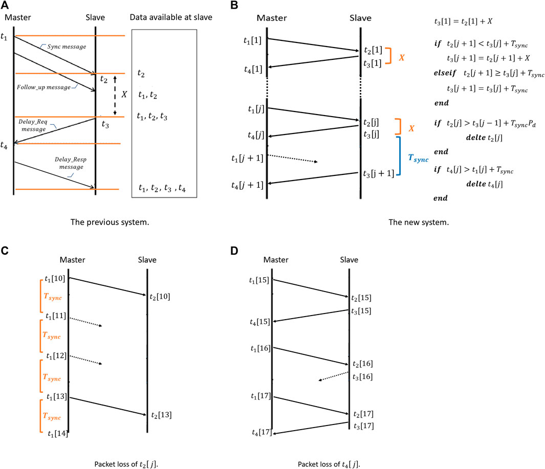
FIGURE 1. PTP message diagram.

In practical systems, a load in the Network or a Cyber-attack may cause packet loss. The packet loss can occur in the Forward and Reverse paths. When the packet loss occurs in the Forward path, we may have three types of messages that may get lost: 1.) The Sync message 2.) The Follow-up message 3.) The Delay Resp message. It should be pointed out that when the Sync message gets lost (meaning that the Slave has a missing time stamp of t₂[j]), the Slave cannot send back the Delay Req message to the Master since it should send the Delay Req message after the constant time (X) from t₂[j] (please refer to Figure 1A). In general, lost messages from the Forward path cause missing messages in the Reverse path. In order to avoid the case where lost messages in the Forward path cause missing messages in the Reverse path, we define a new system described in Figure 1B. For the first Sync period, the Slave must receive a Sync message (t₂[1]) to begin the synchronization process. After the first Sync message has been received by the Slave, the Slave sends the first Delay Req message after a constant time of t₃[1] = t₂[1] + X. Then, the Slave waits for a period of time t₃[j − 1] + T_sync in order to receive the Sync message at the time stamp t₂[j] from the Master in order to send the Master its Delay Req message at the time stamp t₃[j]. Note that from this stage, the Slave has, according to our new proposed system (Figure 1B) two options for sending out the Delay Req message at the time stamp t₃[j].

1) If the Sync message at time stamp t₂ [j] is received before the end of the time t₃[j − 1] + T_sync, then the Slave sends the Delay Req message at time stamp t₃[j] as usual after a constant time from t₂[j], namely, t₃[j] = t₂[j] + X.

2) If the Sync message at time stamp t₂[j] is not received until the end of this duration (t₃[j − 1] + T_sync), then the Slave sends the Delay Req message at time stamp t₃[j] equivalent to t₃[j] = t₃[j − 1] + T_sync.

If the Slave does not receive the Sync message at the time stamp t₂[j] or the Delay Resp message at the time stamp t₄[j] or even both of them, then those time stamps (t₂[j], t₄[j]) are going to be estimated as will be shown in Section 3. Note, when the missing messages are the Follow-up messages (containing t₁[j]), the missing time stamps of t₁[j] can be obtained via the knowledge that the difference between two consecutive Sync time stamps is a constant time of T_sync. For example, if the time stamps t₁ [j] and t₁[j + 1] are missing, we can write: t₁[j] = t₁[j − 1] + T_sync and t₁[j + 1] = t₁[j − 1] + 2T_sync. In the new system (described in Figure 1B), we also use two additional conditions in the Slave in order to block too noisy packets.

1) if (t₂[j] > t₃[j − 1] + T_syncP_d) delete t₂[j].

2) if (t₄[j] > t₁[j] + T_sync) delete t₄[j].

In our simulation, we set P_d = 1.5.

In the following section, we estimate t₂[j] and t₄[j] for the case that they are missing at the Slave.

3 Estimating the missing time stamps

This section estimates the missing time stamps t₂[j] and t₄[j]. In the following, we denote the estimated t₂[j] as ${\widehat{t}}_2[j]$ and define it by:

${\widehat{t}}_2\left[S_i+L-1\right]=t_2\left[S_i-1\right]+\frac{L}{K_i+1}\left(t_2\left[S_i+K_i\right]-t_2\left[S_i-1\right]\right)(3)$

where K is a vector with elements K_i, K = [K₁, K₂, K₃, … , K_i, … ] and where K_i indicates the length of a group of consecutive missing time stamps of t₂[j]. For example, when K = [2, 1], it means that K₁ = 2; the first group has two consecutive missing time stamps. For the second group, K₂ = 1, meaning this group has only one missing time stamp. S is a vector with elements S_i, S = [S₁, S₂, S₃, … , S_i, … ] where S_i indicates the position of the first missing consecutive time stamp of t₂[j]. For example, when S = [10, 24], S₁ = 10, the first group of the consecutive missing time stamps starts at j = 10. The second group starts at j = 24 since S₂ = 24. The following variable L is defined as L = 1, 2, … K_i. The time stamp t₂[S_i − 1] denotes the time stamp of t₂[j] that comes before the missing time stamps. The time stamp t₂[S_i + K_i] denotes the time stamp of t₂[j] that comes after the missing time stamps, and $\frac{1}{K_i+1}(t_2[S_i+K_i]-t_2[S_i-1])$ denotes the average time between those time stamps (we can average this factor since the difference between two consecutive time stamps of Sync messages is T_sync). For example, when K = [2, 1, 3, 4] and S = [11, 21, 43, 52], we have four groups of missing consecutive messages in different places ([K_i, S_i]: [2, 11], [1, 21], [3, 43], [4, 52]). We have two missing time stamps for the first group at j = 11 and j = 12. For K₁ = 2, we can write that L = 1, 2. Please refer to Figure 1C where the reconstruction of the first group can be written based on (3) as follows:

${\widehat{t}}_2\left[11\right]=t_2\left[10\right]+\frac{1}{3}\left(t_2\left[13\right]-t_2\left[10\right]\right),L=1$

and

${\widehat{t}}_2\left[12\right]=t_2\left[10\right]+\frac{2}{3}\left(t_2\left[13\right]-t_2\left[10\right]\right),L=2$

The estimated missing time stamp of t₄[j] is denoted as ${\widehat{t}}_4[j]$. Unlike (3) where the difference between two consecutive time stamps of Sync messages is constant, the difference between two consecutive time stamps of Delay Req messages changes over time. Therefore, it is necessary to apply also the time stamp of t₃[j] in the estimation of t₄[j]. ${\widehat{t}}_4[j]$ is given by:

${\widehat{t}}_4\left[{\tilde{S}}_i+\tilde{L}-1\right]={\widehat{t}}_4\left[{\tilde{S}}_i+\tilde{L}-2\right]+\left(t_4\left[{\tilde{S}}_i+{\tilde{K}}_i\right]-t_4\left[{\tilde{S}}_i-1\right]\right)N\left({\tilde{S}}_i,{\tilde{K}}_i,\tilde{L}\right)(4)$

where $\tilde{K}$ is a vector with elements ${\tilde{K}}_i$, $\tilde{K}=[{\tilde{K}}_1,{\tilde{K}}_2,{\tilde{K}}_3,\dots ,{\tilde{K}}_i,\dots ]$ and where ${\tilde{K}}_i$ indicates the length of a group of consecutive missing packets of t₄ [.] $\tilde{S}$ is a vector with elements ${\tilde{S}}_i$, $\tilde{S}=[{\tilde{S}}_1,{\tilde{S}}_2,{\tilde{S}}_3,\dots ,{\tilde{S}}_i,\dots ]$ where ${\tilde{S}}_i$ indicates the position of the first missing consecutive time stamp of t₄ [.] In the following, the variable $\tilde{L}$ is defined as $\tilde{L}=\mathrm{1,2},.{\tilde{K}}_i$, where the function $N({\tilde{S}}_i,{\tilde{K}}_i,\tilde{L})$ is:

$N\left({\tilde{S}}_i,{\tilde{K}}_i,\tilde{L}\right)=\frac{t_3\left[{\tilde{S}}_i+\tilde{L}-1\right]-t_3\left[{\tilde{S}}_i+\tilde{L}-2\right]}{t_3\left[{\tilde{S}}_i+{\tilde{K}}_i\right]-t_3\left[{\tilde{S}}_i-1\right]}(5)$

Please note, the time stamp $t_4[{\tilde{S}}_i-1]$ denotes the time stamp of t₄ [j] that comes before the missing time stamps; the time stamp $t_4[{\tilde{S}}_i+{\tilde{K}}_i]$ denotes the time stamp of t₄ [j] that comes after the missing time stamps. For example, when $\tilde{K}=[\mathrm{1,4,3,2}]$ and $\tilde{S}=[\mathrm{16,33,41,62}]$, we have four groups of missing consecutive messages in different places $([{\tilde{K}}_i,{\tilde{S}}_i]:[\mathrm{1,16}],[\mathrm{4,33}],[\mathrm{3,41}],[\mathrm{2,62}])$. We have one missing time stamp for the first group at j = 16. For ${\tilde{K}}_1=1$ we can write that $\tilde{L}=1$, please refer to Figure 1D. The reconstruction of the first group can be written based on (4) and (5) as follows:

${\widehat{t}}_4\left[16\right]=t_4\left[15\right]+\left(t_4\left[17\right]-t_4\left[15\right]\right)\frac{t_3\left[16\right]-t_3\left[15\right]}{t_3\left[17\right]-t_3\left[15\right]},\tilde{L}=1$

4 The modified clock skew estimators applicable for the packet loss/non-packet loss case

In our previous works [2, 3 and 14], we presented three clock skew estimators, one for the TWD case [2] and two for the OWD case [3] (for the Forward and Reverse paths). Those clock skew estimators will show a degradation in the clock skew performance when packet loss occurs. A reduction in the clock skew performance is also shown in other clock skew estimators, such as with the MLLE clock skew estimator [12] or with the Kalman clock skew estimator [15]. In order to make them work efficiently in the packet loss environment, we modify the three clock skew estimators [2], [3] in such a way that they will also work efficiently for the packet loss case.

4.1 Theorem 1

The TWD clock skew estimator from [2] is in the following modified to answer also for the packet loss case and is given by:

$\widehat{\alpha }=\frac{1}{J\left(J-1\right)}{\displaystyle \sum _{i=1}^{J-1}}{\displaystyle \sum _{j=1}^{J-i}}\left(\frac{T_{1,j}\left(i\right)}{{\widehat{T}}_{2,j}\left(i\right)}+\frac{{\widehat{T}}_{4,j}\left(i\right)}{T_{3,j}\left(i\right)}\right)-1(6)$

where $\widehat{\alpha }$ is the estimated clock skew and for l = 1, 3 we may express T_l,j(i) as:

$T_{l,j}\left(i\right)=t_l\left[j+i\right]-t_l\left[j\right](7)$

and ${\widehat{T}}_{\tilde{l},j}(i)$ is given for $\tilde{l}=\mathrm{2,4}$ by:

${\widehat{T}}_{\tilde{l},j}\left(i\right)={\widehat{t}}_{\tilde{l}}\left[j+i\right]-{\widehat{t}}_{\tilde{l}}\left[j\right](8)$

If during a Sync period, the time stamps t₂[j] or t₄[j] or both of them are missing, we estimate them $({\widehat{t}}_{\tilde{l}}[j])$ based on (3) or (4), otherwise no estimation is needed and in this case, we have ${\widehat{t}}_{\tilde{l}}[j]=t_{\tilde{l}}[j]$. The OWD clock skew estimators for the Forward and Reverse paths from [3] are modified to answer also for the packet loss case and can be written as:

${\widehat{\alpha }}_F=\frac{2}{J\left(J-1\right)}{\displaystyle \sum _{i=1}^{J-1}}{\displaystyle \sum _{j=1}^{J-i}}\left(\frac{T_{1,j}\left(i\right)}{{\widehat{T}}_{2,j}\left(i\right)}\right)-1(9)$

and

${\widehat{\alpha }}_R=\frac{2}{J\left(J-1\right)}{\displaystyle \sum _{i=1}^{J-1}}{\displaystyle \sum _{j=1}^{J-i}}\left(\frac{{\widehat{T}}_{4,j}\left(i\right)}{T_{3,j}\left(i\right)}\right)-1(10)$

where ${\widehat{\alpha }}_F$ and ${\widehat{\alpha }}_R$ are the estimated clock skews for the Forward and Reverse paths, respectively.

4.1.1 Proof of Theorem 1

The proof is given in the appendix.

5 The MSE upper bound for the modified clock skew estimators

By having on hand the MSE expressions, the system designer can know the total number of Sync periods needed to answer the system’s performance requirement from the MSE point of view. Thus, it could be helpful to have closed-form approximated expressions for the MSE related to the proposed clock skew estimators (6), (9) and (10) under the packet loss case. In [2] and [3], we assumed to have all the PTP packets to derive the closed-form approximated expressions for the MSE. However, in the packet loss case, we have to estimate the missing time stamps according to (3) and (4). Therefore, it is not easy to derive the closed-form approximated expressions for the MSE related to the proposed modified clock skew estimators. In the following, we derive the upper bounds for the closed-form approximated expressions for the MSE related to the modified TWD clock skew estimator and OWD clock skew estimators for the Forward and Reverse paths ((6); (9); (10)) for the packet loss case. The approximated MSE upper bounds are applicable for the fGn case with packet loss and in the presence of asymmetry in the fixed delays, asymmetry in the PDVs, or even asymmetry in the Hurst exponent parameters between the Forward and Reverse paths.

5.1 Assumptions

In the following, we assume that the PTP system operates in an fGn environment (including the Gaussian case); the PDV is a zero-mean process with the Hurst exponent parameter (H) in the range of 0.5 ≤ H < 1. The PDV variance for j = i is:

$E\left[{\omega }_n\left(i\right){\omega }_n\left(j\right)\right]={\sigma }_{{\omega }_n}^2(11)$

When i ≠ j, the PDV variance is given by [16] and [17]:

$E\left[{\omega }_n\left(i\right){\omega }_n\left(j\right)\right]=\frac{{\sigma }_{{\omega }_n}^2}{2}\left[{\left|{\left|i-j\right|}^a-1\right|}^{2H_p}-2{\left({\left|i-j\right|}^a\right)}^{2H_p}+{\left({\left|i-j\right|}^a+1\right)}^{2H_p}\right](12)$

where for n = 1, 2 and p = F, R, respectively. H_F and H_R are the Hurst exponent parameters for the Forward and Reverse paths, respectively. Note that the a parameter is related to the gfGn case. In this work, we set a = 1 for the gfGn case (thus considering only the fGn case).

5.2 Theorem 1

The approximated MSE upper bound expression for the modified TWD clock skew estimator (6) with packet loss is:

$\begin{array}{cc}\hfill E\left[e^2\right]& \approx \frac{G_{\mathit{TWD}}}{{\left(2\left(J-1\right)T_{\mathit{syn}}\right)}^2}\left(1+\frac{1}{\tilde{P}}\right)\left({\sigma }_{{\omega }_1}^2\left(2-{\left(J-2\right)}^{2H_F}+2{\left(J-1\right)}^{2H_F}-{\left(J\right)}^{2H_F}\right)\right.\hfill \\ \hfill & \left.+{\sigma }_{{\omega }_2}^2\left(2-{\left(J-2\right)}^{2H_R}+2{\left(J-1\right)}^{2H_R}-{\left(J\right)}^{2H_R}\right)\right)\hfill \\ \hfill & +\frac{\left(1-G_{\mathit{TWD}}\right)}{{\left(J\left(J-1\right)T_{\mathit{syn}}\right)}^2}\left({\sigma }_{{\omega }_1}^2+\overline{{\sigma }_{{\omega }_2}^2}\right)\left(\left(1+\frac{1}{P}\right)C\left(J,H_F\right)+D\left(J,H_F\right)\right)\hfill \end{array}(13)$

$\tilde{P}$ is given by:

$\tilde{P}=\frac{\left({\sigma }_{{\omega }_1}^2+{\sigma }_{{\omega }_2}^2\right)}{6{\sigma }_{{\omega }_1}^4}{\left(J-1\right)}^2{T}_{\mathit{syn}}^2(14)$

where P, A, B, C, and D are given by [2]:

$P=\frac{A}{B}\left(\frac{{\sigma }_{{\omega }_1}^2+{\sigma }_{{\omega }_2}^2}{{\sigma }_{{\omega }_1}^4}\right)T_{\mathit{syn}}^2(15)$

$A=\left(2{\displaystyle \sum _{i=1}^{J-1}}\frac{J-i}{i^2}+{\displaystyle \sum _{i=1}^{J-1}}{\displaystyle \sum _{j=1}^{J-i}}{\displaystyle \sum _{\begin{array}{c}k=1\\ k\ne i\end{array}}^{J-1}}{\displaystyle \sum _{\begin{array}{c}m=1\\ m=j\\ m=j+i-k\end{array}}^{J-k}}\frac{1}{ik}-{\displaystyle \sum _{i=1}^{J-1}}{\displaystyle \sum _{j=1}^{J-i}}{\displaystyle \sum _{\begin{array}{c}k=1\end{array}}^{J-1}}{\displaystyle \sum _{\begin{array}{c}m=1\\ m=j+i\\ m=j-k\end{array}}^{J-k}}\frac{1}{ik}\right)(16)$

$B=\left(12{\displaystyle \sum _{i=1}^{J-1}}\frac{J-i}{i^4}+6{\displaystyle \sum _{i=1}^{J-1}}{\displaystyle \sum _{j=1}^{J-i}}{\displaystyle \sum _{\begin{array}{c}k=1\\ k\ne i\end{array}}^{J-1}}{\displaystyle \sum _{\begin{array}{c}m=1\\ m=j\\ m=j+i-k\\ m=j+i\\ m=j-k\end{array}}^{J-k}}\frac{1}{{\left(ik\right)}^2}+4{\displaystyle \sum _{i=1}^{J-1}}{\displaystyle \sum _{j=1}^{J-i}}{\displaystyle \sum _{\begin{array}{c}k=1\end{array}}^{J-1}}{\displaystyle \sum _{\begin{array}{c}m=1\\ m\ne j\\ m\ne j+i-k\\ m\ne j+i\\ m\ne j-k\end{array}}^{J-k}}\frac{1}{{\left(ik\right)}^2}\right)(17)$

$\begin{array}{cc}\hfill C& ={\displaystyle \sum _{i=1}^{J-1}}\frac{J-i}{i^2}\left(2-f{G}_H^{*}\left(i,H_p,a\right)\right)\hfill \\ \hfill & +{\displaystyle \sum _{i=1}^{J-1}}{\displaystyle \sum _{j=1}^{J-i}}{\displaystyle \sum _{\begin{array}{c}k=1\\ k\ne i\end{array}}^{J-1}}{\displaystyle \sum _{\begin{array}{c}m=1\\ m=j\\ m=j+i-k\end{array}}^{J-k}}\frac{1}{ik}(1+\frac{1}{2}(f{G}_{\begin{array}{c}H\end{array}}^{*}\left(i-k,H_p,a\right)-f{G}_H^{*}\left(i,H_p,a\right)-f{G}_H^{*}\left(k,H_p,a\right)))\hfill \\ \hfill & -{\displaystyle \sum _{i=1}^{J-1}}{\displaystyle \sum _{j=1}^{J-i}}{\displaystyle \sum _{\begin{array}{c}k=1\end{array}}^{J-1}}{\displaystyle \sum _{\begin{array}{c}m=1\\ m=j+i\\ m=j-k\end{array}}^{J-k}}\frac{1}{ik}(1-\frac{1}{2}(f{G}_H^{*}\left(i,H_p,a\right)-f{G}_H^{*}\left(k,H_p,a\right)+f{G}_H^{*}\left(i+k,H_p,a\right)))\hfill \end{array}(18)$

$\begin{array}{cc}\hfill D& ={\displaystyle \sum _{i=1}^{J-1}}{\displaystyle \sum _{j=1}^{J-i}}{\displaystyle \sum _{\begin{array}{c}k=1\end{array}}^{J-1}}{\displaystyle \sum _{\begin{array}{c}m=1\\ m\ne j\\ m\ne j+i\\ m\ne j-k\\ m\ne j+i-k\end{array}}^{J-k}}\frac{1}{2ik}\left(f{G}_H^{*}\left(j-m,H_p,a\right)-f{G}_H^{*}\left(j+i-m,H_p,a\right)\right.\hfill \\ \hfill & \left.-f{G}_H^{*}\left(j-m-k,H_p,a\right)+f{G}_H^{*}\left(j+i-m-k,H_p,a\right)\right)\hfill \end{array}(19)$

And the function $f{G}_H^{*}(.)$ is given by [2]:

$f{G}_H^{*}\left(x,H_p,a\right)=\left[\Vert x^a|-1{|}^{2H_p}-2{\left(|x^a|\right)}^{2H_p}+{\left(|x^a|+1\right)}^{2H_p}\right](20)$

where p = F, R.

Please note that in [2] H_F = H_R = H since we assumed that both paths have the same Hurst exponent parameters. We also have $\overline{{\sigma }_{{\omega }_2}^2}={\sigma }_{{\omega }_2}^2\tilde{S}$, where $\tilde{S}$ is a compensation factor that compensates for the asymmetry between the Hurst exponent parameters for the Forward and Reverse paths. $\tilde{S}$ is given by:

$\tilde{S}=\frac{C\left(J,H_R\right)\left(1+\frac{1}{P}\right)+D\left(J,H_R\right)}{C\left(J,H_F\right)\left(1+\frac{1}{P}\right)+D\left(J,H_F\right)}(21)$

And G_TWD is a weight function for the approximated MSE upper bound related to the TWD case (6) and is defined by:

$\begin{array}{cc}\hfill & \text{if\hspace{0.17em}}{P}_{M_F}\ne \text{\hspace{0.17em}0\hspace{0.17em}and\hspace{0.17em}}{P}_{M_R}\ne \text{\hspace{0.17em}0}\hfill \\ \hfill & G_{\mathit{TWD}}=\left(\frac{2}{J\left(1-\frac{P_{M_F}}{3}-P_{M_R}\right)}\right)\mathit{max}\left(R_F,R_R\right)\hfill \\ \hfill & \text{else\hspace{0.17em}if\hspace{0.17em}}{P}_{M_F}\ne \text{\hspace{0.17em}0}\hfill \\ \hfill & G_{\mathit{TWD}}=\frac{2}{J\left(1-\frac{P_{M_F}}{3}\right)}{R}_F\hfill \\ \hfill & \text{else\hspace{0.17em}if\hspace{0.17em}}{P}_{M_R}\ne \text{\hspace{0.17em}0}\hfill \\ \hfill & G_{\mathit{TWD}}=\frac{2}{J\left(1-P_{M_R}\right)}{R}_R\hfill \\ \hfill & \text{else}\hfill \\ \hfill & G_{\mathit{TWD}}=0\hfill \end{array}(22)$

where $P_{M_F}$ and $P_{M_R}$ are denoted as the packet loss percentage in the Forward and Reverse paths, respectively $(0\le P_{M_F},P_{M_R}<1)$, and max(., .) is the maximum function. The parameters R_F and R_R are correction parameters that are applied in the case where the missing packets appear as short bursts instead of being randomly distributed over time. The correction parameters R_F and R_R are set by the user and are defined as:

$R_F=r+r_F\left(\frac{J}{4}\frac{P_{M_F}}{3}\right)(23)$

And

$R_R=r+r_R\left(\frac{J{P}_{M_R}}{4}\right)(24)$

where r is a positive parameter. In our simulations, we set r = 2. If we set a higher value for r, we will get a higher approximated upper bound for the MSE, and on the contrary, if we set a lower value for r, the approximated upper bound for the MSE will be lower. The system designer sets the variables r_F and r_R in the range of 0 ≤ r_F, r_R ≤ 1. When the system designer assumes that the packet loss is randomly distributed over time, he sets r_F = 0 or r_R = 0. However, if the system designer assumes that all the missing packets at the Forward or Reverse paths appear at one burst, he sets r_F = 1 or r_R = 1. Note that the system designer has to set the parameters: $P_{M_F}$, $P_{M_R}$, r_F, and r_R, in order to apply the approximated upper bound for the MSE related to the TWD clock skew estimator (6). Those parameters ($P_{M_F}$, $P_{M_R}$, r_F, r_R) do not necessarily represent the actual statistics of the ratio of the packet loss for the Forward and Reverse paths but are intended to help the system designer to get approximately the maximum number of Sync periods needed to obtain the system’s requirement.

5.2.1 Proof of Theorem 1

In order to derive the approximated upper bound related to the TWD clock skew estimator (6), we apply two different cases. The first is case A when the Slave has no missing packets, as shown in [2] and [3]. The second is case B when all the packets are lost except those related to the first and last Sync periods, as will be shown in the following. The approximated MSE upper bound will be the summation of case A and case B with different weights. Let us recall from [2] the general expression for the approximated MSE related to the TWD clock skew estimator:

$\begin{array}{cc}\hfill E\left[e^2\right]& \approx {\left(\frac{1}{\left(J\left(J-1\right)\right)T_{\mathit{syn}}}\right)}^2{\displaystyle \sum _{i=1}^{J-1}}{\displaystyle \sum _{j=1}^{J-i}}{\displaystyle \sum _{k=1}^{J-1}}{\displaystyle \sum _{m=1}^{J-k}}\left[\frac{E\left[{\mathrm{\Omega }}_{1,j}\left(i\right){\mathrm{\Omega }}_{1,m}\left(k\right)\right]}{ik}+\frac{E\left[{\mathrm{\Omega }}_{2,j}\left(i\right){\mathrm{\Omega }}_{2,m}\left(k\right)\right]}{ik}+\frac{1}{T_{\mathit{syn}}^2}\frac{E\left[{\mathrm{\Omega }}_{1,j}^2\left(i\right){\mathrm{\Omega }}_{1,m}^2\left(k\right)\right]}{{\left(ik\right)}^2}\right]\hfill \end{array}(25)$

where Ω_n,j(i) is:

${\mathrm{\Omega }}_{n,j}\left(i\right)={\omega }_n\left[j+i\right]-{\omega }_n\left[j\right](26)$

For case B, we have only the first and the last Sync periods, where based on (26) Ω_n,1 (J − 1) = ω_n [J] − ω_n [1]. In (25) as we have shown in [2], we have $\frac{J(J-1)}{2}$ cases for the expression Ω_n,j(i) for J Sync periods. However, in case B, we have only one case. Therefore, (25) can be written for case B as:

$\begin{array}{cc}\hfill E\left[e^2\right]& \approx {\left(\frac{1}{2T_{\mathit{syn}}}\right)}^2\left[\frac{E\left[{\mathrm{\Omega }}_{\mathrm{1,1}}\left(J-1\right){\mathrm{\Omega }}_{\mathrm{1,1}}\left(J-1\right)\right]}{{\left(J-1\right)}^2}+\frac{E\left[{\mathrm{\Omega }}_{\mathrm{2,1}}\left(J-1\right){\mathrm{\Omega }}_{\mathrm{2,1}}\left(J-1\right)\right]}{{\left(J-1\right)}^2}\right.\hfill \\ \hfill & \left.+\frac{1}{T_{\mathit{syn}}^2}\frac{E\left[{\mathrm{\Omega }}_{\mathrm{1,1}}^2\left(J-1\right){\mathrm{\Omega }}_{\mathrm{1,1}}^2\left(J-1\right)\right]}{{\left(J-1\right)}^4}\right]\hfill \end{array}(27)$

By substituting (26) into (27) we may write:

$\begin{array}{cc}E\left[e^2\right]\hfill & \approx {\left(\frac{1}{2\left(J-1\right)T_{\mathit{syn}}}\right)}^2[E[{\omega }_1^2\left[J\right]]+E\left[{\omega }_1^2\left[1\right]\right]-2E\left[{\omega }_1\left[1\right]{\omega }_1\left[J\right]\right]]\hfill \\ \hfill & +E\left[{\omega }_2^2\left[J\right]\right]+E\left[{\omega }_2^2\left[1\right]\right]-2E\left[{\omega }_2\left[1\right]{\omega }_2\left[J\right]\right]+\frac{E\left[{\omega }_1^4\left[J\right]\right]+E\left[{\omega }_1^4\left[1\right]\right]+6E\left[{\omega }_1^2\left[1\right]{\omega }_1^2\left[J\right]\right]}{{\left(\left(J-1\right)T_{\mathit{syn}}\right)}^2}\left.-\frac{4E\left[{\omega }_1\left[1\right]{\omega }_1^3\left[J\right]\right]+4E\left[{\omega }_1^3\left[1\right]{\omega }_1\left[J\right]\right]}{{\left(\left(J-1\right)T_{\mathit{syn}}\right)}^2}\right]\hfill \end{array}(28)$

By setting $E[{\omega }_1[1]{\omega }_1^3[J]]$ and $E[{\omega }_1^3[1]{\omega }_1[J]]$ to zero, the expression in (28) can be written as:

$\begin{array}{cc}\hfill E\left[e^2\right]& \approx {\left(\frac{1}{2\left(J-1\right)T_{\mathit{syn}}}\right)}^2[\left(E\left[{\omega }_1^2\left[J\right]\right]+E\left[{\omega }_1^2\left[1\right]\right]-2E\left[{\omega }_1\left[1\right]{\omega }_1\left[J\right]\right]\right)\hfill \\ \hfill & +\left(E\left[{\omega }_2^2\left[J\right]\right]+E\left[{\omega }_2^2\left[1\right]\right]-2E\left[{\omega }_2\left[1\right]{\omega }_2\left[J\right]\right]\right)+\left(\frac{E\left[{\omega }_1^4\left[J\right]\right]+E\left[{\omega }_1^4\left[1\right]\right]+6E\left[{\omega }_1^2\left[1\right]{\omega }_1^2\left[J\right]\right]}{{\left(\left(J-1\right)T_{\mathit{syn}}\right)}^2}\right)]\hfill \end{array}(29)$

Based on the assumption made in (11) we may write (29) for the Gaussian case (H = 0.5) as:

$E\left[e^2\right]\approx {\left(\frac{1}{2\left(J-1\right)T_{\mathit{syn}}}\right)}^2\left[2{\sigma }_{{\omega }_1}^2+2{\sigma }_{{\omega }_2}^2+\frac{1}{{\left(\left(J-1\right)T_{\mathit{syn}}\right)}^2}\left(6{\sigma }_{{\omega }_1}^4+6{\sigma }_{{\omega }_1}^2{\sigma }_{{\omega }_1}^2\right)\right](30)$

After rearranging (30), we have for the Gaussian case (H = 0.5):

$E\left[e^2\right]\approx {\left(\frac{1}{2\left(J-1\right)T_{\mathit{syn}}}\right)}^2\left[2\left({\sigma }_{{\omega }_1}^2+{\sigma }_{{\omega }_2}^2\right)\left(1+\frac{1}{\tilde{P}}\right)\right](31)$

where $\tilde{P}$ is defined in (14).For the fGn case (0.5 ≤ H < 1), based on the assumptions made in (11) and (12), we may write the two first parts in the square brackets in (29) as:

$E\left[{\omega }_n^2\left[J\right]\right]+E\left[{\omega }_n^2\left[1\right]\right]-2E\left[{\omega }_n\left[1\right]{\omega }_n\left[J\right]\right]=2{\sigma }_{{\omega }_n}^2-{\sigma }_{{\omega }_n}^2\left({\left(J-2\right)}^{2H_p}-2{\left(J-1\right)}^{2H_p}+{\left(J\right)}^{2H_p}\right)(32)$

The third part in the square brackets in (29) is quite challenging for the fGn case. In [2], we had a similar difficulty with a different expression. Thus, we will apply here the same technique as was used in [2] to calculate the challenging part here. Therefore, by using the same technique applied in [2], we multiply the sum of the first two parts in the square brackets in (29) with the factor $(1+\frac{1}{\tilde{P}})$. Please note that $\tilde{P}$ (14) is obtained by dividing the sum of the first two parts in the square brackets in (30) by the third part in the square brackets in (30) for the Gaussian case. Therefore, in case B, the general expression for the approximated MSE related to the TWD clock skew estimator for the fGn case can be written as:

$\begin{array}{cc}\hfill E\left[e^2\right]& \approx {\left(\frac{1}{2\left(J-1\right)T_{\mathit{syn}}}\right)}^2\left(1+\frac{1}{\tilde{P}}\right)\left[{\sigma }_{{\omega }_1}^2\left(2-{\left(J-2\right)}^{2H_F}+2{\left(J-1\right)}^{2H_F}-{\left(J\right)}^{2H_F}\right)\right.\hfill \\ \hfill & \left.+{\sigma }_{{\omega }_2}^2\left(2-{\left(J-2\right)}^{2H_R}+2{\left(J-1\right)}^{2H_R}-{\left(J\right)}^{2H_R}\right)\right]\hfill \end{array}(33)$

For case A, let us recall from [2] the general expression for the approximated MSE related to the TWD clock skew estimator for the fGn case:

$E\left[e^2\right]\approx \frac{\left({\sigma }_{{\omega }_1}^2+{\sigma }_{{\omega }_2}^2\right)}{{\left(J\left(J-1\right)T_{\mathit{syn}}\right)}^2}\left(\left(1+\frac{1}{P}\right)C+D\right)(34)$

In [2], we assumed that we have the same Hurst exponent parameter for the Forward and Reverse paths (H_F = H_R), but in this work, we also consider the case where H_R ≠ H_F. Therefore, we have to apply the compensation factor in (21). In this case, we set the Hurst exponent parameter for the Forward path (H_F) for C (18) and D (19), and we also multiply the PDV variance of the Reverse path with the compensation factor $(\overline{{\sigma }_{{\omega }_2}^2}={\sigma }_{{\omega }_2}^2\tilde{S})$. Therefore, we can write (34) as:

$E\left[e^2\right]\approx \frac{\left({\sigma }_{{\omega }_1}^2+\overline{{\sigma }_{{\omega }_2}^2}\right)}{{\left(J\left(J-1\right)T_{\mathit{syn}}\right)}^2}\left(\left(1+\frac{1}{P}\right)C\left(J,H_F\right)+D\left(J,H_F\right)\right)(35)$

Up to now, we have the two general expressions for the approximated MSE related to the TWD clock skew estimator for two cases, case A given by (35), and the second case B as shown in (33). In order to derive the approximated MSE upper bound, we have to define the weight function that sums those two general expressions for the approximated MSE. The weight function (G_TWD) is applied for case B, where for case A we apply (1 − G_TWD). The weight function G_TWD depends on the two parameters $P_{M_F}$ and $P_{M_R}$. Thus, we have four options for the setting G_TWD:

Option 1: When we have all the PTP packets $(P_{M_F}=P_{M_R}=0)$, we set G_TWD = 0. In this case, we have only the general expressions for the approximated MSE related to the TWD clock skew estimator for case A.

Option 2: When we have packet loss only in the Forward path ($P_{M_F}\ne 0$ and $P_{M_R}=0$). In this case, we have approximately $J(1-P_{M_F}/3)$ time stamps (of t₂ [j] or t₄ [j]) in the Forward path, and in case B we have two Sync periods. The parameter R_F increases the ratio between those numbers and gives more weight to the approximated MSE of case B. Therefore, if we set a higher value for R_F, we will get a higher approximated upper bound for the MSE. In this case, we can set $G_{\mathit{TWD}}=\frac{2}{J(1-P_{M_F}/3)}{R}_F$.

Option 3: When we have packet loss only in the Reverse path ($P_{M_F}=0$ and $P_{M_R}\ne 0$). In this case, in the Reverse path, we have approximately $J(1-P_{M_R})$ time stamps (of t₄ [j]), and in case B, we have two Sync periods. The parameter R_R increases the ratio between those numbers and gives more weight to the approximated MSE of case B. Therefore, if we set a higher value for R_R, we will get a higher approximated upper bound for the MSE. In this case, we can set $G_{\mathit{TWD}}=\frac{2}{J(1-P_{M_R})}{R}_R$.

Option 4: When we have packet loss in both paths ($P_{M_F}\ne 0$ and $P_{M_R}\ne 0$). In this case, we may have approximately $J(1-P_{M_F}/3-P_{M_R})$ time stamps (of t₂ [j] or t₄ [j]). Note that we assume that the missing time stamps in the Forward path are at a different Sync period than those in the Reverse path. Therefore, we set $G_{\mathit{TWD}}=\frac{2}{J(1-P_{M_F}/3-P_{M_R})}\mathit{max}(R_F,R_R)$.

By using the weight function (22) together with (33) and (35), we can get the MSE upper bound in (13), and this completes our proof.

5.3 Theorem 2

The approximated MSE upper bound expression for the modified OWD clock skew estimator for the Forward path (9) with packet loss is:

$\begin{array}{cc}\hfill E\left[e_F^2\right]& \approx \frac{G_{OW{D}_F}}{{\left(\left(J-1\right)T_{\mathit{syn}}\right)}^2}\left(1+\frac{1}{{\tilde{P}}_F}\right)\left({\sigma }_{{\omega }_1}^2\left(2-{\left(J-2\right)}^{2H_F}+2{\left(J-1\right)}^{2H_F}-{\left(J\right)}^{2H_F}\right)\right)\hfill \\ \hfill & +\frac{4{\sigma }_{{\omega }_1}^2\left(1-G_{OW{D}_F}\right)}{{\left(J\left(J-1\right)T_{\mathit{syn}}\right)}^2}\left(\left(1+\frac{1}{P_F}\right)C\left(J,H_F\right)+D\left(J,H_F\right)\right)\hfill \end{array}(36)$

where ${\tilde{P}}_F$ is:

${\tilde{P}}_F=\frac{{\left(J-1\right)}^2{T}_{\mathit{syn}}^2}{6{\sigma }_{{\omega }_1}^2}(37)$

And P_F is given by [3] as:

$P_F=\frac{A}{B}\left(\frac{T_{\mathit{syn}}^2}{{\sigma }_{{\omega }_1}^2}\right)(38)$

where $G_{OW{D}_F}$ is the weight function in the approximated MSE upper bound expression related to the OWD for the Forward path case (9) and is defined as:

$\begin{array}{cc}\hfill & \text{if\hspace{0.17em}}{P}_{M_F}\ne \text{\hspace{0.17em}0}\hfill \\ \hfill & G_{OW{D}_F}=\frac{2}{J\left(1-\frac{P_{M_F}}{3}\right)}{R}_F\hfill \\ \hfill & \text{else}\hfill \\ \hfill & G_{OW{D}_F}=0\hfill \end{array}(39)$

5.4 Proof of Theorem 2

In order to derive the approximated MSE upper bound related to the OWD clock skew estimator for the Forward path (9), we also apply here case A and case B. The MSE upper bound is the summation of these two cases with different weights.

Let us recall from [3] the general expression for the approximated MSE related to the OWD clock skew estimator for the Forward path:

$E\left[e_F^2\right]\approx {\left(\frac{2}{\left(J\left(J-1\right)\right)T_{\mathit{syn}}}\right)}^2{\displaystyle \sum _{i=1}^{J-1}}{\displaystyle \sum _{j=1}^{J-i}}{\displaystyle \sum _{k=1}^{J-1}}{\displaystyle \sum _{m=1}^{J-k}}\left[\frac{E\left[{\mathrm{\Omega }}_{1,j}\left(i\right){\mathrm{\Omega }}_{1,m}\left(k\right)\right]}{ik}+\frac{1}{T_{\mathit{syn}}^2}\frac{E\left[{\mathrm{\Omega }}_{1,j}^2\left(i\right){\mathrm{\Omega }}_{1,m}^2\left(k\right)\right]}{{\left(ik\right)}^2}\right](40)$

For case B, as we explained earlier, we have only the first and the last Sync periods. Thus, based on (26) Ω_1,1 (J − 1) = ω₁[J] − ω₁[1]. In (40) as we have shown in [3], we have $\frac{\left(J(J-1)\right.}{2}$ cases for the expression Ω_1,j(i) for J Sync periods. However, in case B, we have only one case. Therefore, (40) can be written for case B as:

$E\left[e_F^2\right]\approx {\left(\frac{1}{T_{\mathit{syn}}}\right)}^2\left[\frac{E\left[{\mathrm{\Omega }}_{\mathrm{1,1}}\left(J-1\right){\mathrm{\Omega }}_{\mathrm{1,1}}\left(J-1\right)\right]}{{\left(J-1\right)}^2}+\frac{1}{T_{\mathit{syn}}^2}\frac{E\left[{\mathrm{\Omega }}_{\mathrm{1,1}}^2\left(J-1\right){\mathrm{\Omega }}_{\mathrm{1,1}}^2\left(J-1\right)\right]}{{\left(J-1\right)}^4}\right](41)$

By substituting (26) (Ω_1,1(J − 1) = ω₁[J] − ω₁[1]) into (41) and setting $E[{\omega }_1[1]{\omega }_1^3[J]]$ and $E[{\omega }_1^3[1]{\omega }_1[J]]$ to zero, we may write:

$\begin{array}{cc}\hfill E\left[e_F^2\right]& \approx {\left(\frac{1}{\left(J-1\right)T_{\mathit{syn}}}\right)}^2[\left(E\left[{\omega }_1^2\left[J\right]\right]+E\left[{\omega }_1^2\left[1\right]\right]-2E\left[{\omega }_1\left[1\right]{\omega }_1\left[J\right]\right]\right)\hfill \\ \hfill & \left.+\left(\frac{E\left[{\omega }_1^4\left[J\right]\right]+E\left[{\omega }_1^4\left[1\right]\right]+6E\left[{\omega }_1^2\left[1\right]{\omega }_1^2\left[J\right]\right]}{{\left(\left(J-1\right)T_{\mathit{syn}}\right)}^2}\right)\right]\hfill \end{array}(42)$

Based on (42) and the assumption made in (11), the general expression for the approximated MSE related to the OWD clock skew estimator for the Forward path applicable to the Gaussian case (H = 0.5) for case B is:

$E\left[e_F^2\right]\approx {\left(\frac{1}{\left(J-1\right)T_{\mathit{syn}}}\right)}^2\left[2{\sigma }_{{\omega }_1}^2+\frac{1}{{\left(\left(J-1\right)T_{\mathit{syn}}\right)}^2}\left(6{\sigma }_{{\omega }_1}^4+6{\sigma }_{{\omega }_1}^2{\sigma }_{{\omega }_1}^2\right)\right](43)$

After rearranging (43), we have for the Gaussian case (H = 0.5):

$E\left[e_F^2\right]\approx {\left(\frac{1}{\left(J-1\right)T_{\mathit{syn}}}\right)}^2\left[2\left({\sigma }_{{\omega }_1}^2\right)\left(1+\frac{1}{{\tilde{P}}_F}\right)\right](44)$

Where ${\tilde{P}}_F$ is defined in (37).For the fGn case, the first part in the square brackets in (42) can be written according to (32), for n = 1 and p = F. The general expression for the approximated MSE related to case B for the OWD clock skew estimator for the fGn case can be obtained by using (11) and multiplying the first part in the square brackets in (42) with the factor $(1+\frac{1}{{\tilde{P}}_F})$. Please note that the factor ${\tilde{P}}_F$ (37) is obtained by dividing the first part in the square brackets in (43) by the second part in the square brackets in (43) for the Gaussian case. Thus, based on (44), for case B, the general expression for the approximated MSE related to the OWD clock skew estimators for the Forward path applicable to the fGn case (0.5 ≤ H < 1) is:

$E\left[e_F^2\right]\approx {\left(\frac{1}{\left(J-1\right)T_{\mathit{syn}}}\right)}^2\left(1+\frac{1}{{\tilde{P}}_F}\right)\left[{\sigma }_{{\omega }_1}^2\left(2-{\left(J-2\right)}^{2H_F}+2{\left(J-1\right)}^{2H_F}-{\left(J\right)}^{2H_F}\right)\right](45)$

For case A, let us recall from [3] the general expression for the approximated MSE related to the OWD clock skew estimator for the Forward path applicable to the fGn case:

$E\left[e_F^2\right]\approx \frac{\left(4{\sigma }_{{\omega }_1}^2\right)}{{\left(J\left(J-1\right)T_{\mathit{syn}}\right)}^2}\left(\left(1+\frac{1}{P_F}\right)C+D\right)(46)$

In this case, we apply only the Forward path, and there is no asymmetry issue between the paths, unlike the TWD clock skew estimator. In (46), we set (18) and (19) for C and D, respectively, with the Hurst exponent parameter related to the Forward path (H_F). Therefore, (46) can be written as:

$E\left[e_F^2\right]\approx \frac{\left(4{\sigma }_{{\omega }_1}^2\right)}{{\left(J\left(J-1\right)T_{\mathit{syn}}\right)}^2}\left(\left(1+\frac{1}{P_F}\right)C\left(J,H_F\right)+D\left(J,H_F\right)\right)(47)$

Up to now, we have the two general expressions for the approximated MSE related to the OWD clock skew estimator for the Forward path, for case A (47) and for case B (45). In order to derive the approximated MSE upper bound, we have to define the weight function that sums those two general expressions for the approximated MSE. The weight function $G_{OW{D}_F}$ is applied for case B, whereas for case A we apply $(1-G_{OW{D}_F})$. The weight function $G_{OW{D}_F}$ depends on the parameter $P_{M_F}$. Thus, we have two options for setting the function $G_{OW{D}_F}$:

Option 1: When we have all the PTP packets in the Forward path $(P_{M_F}=0)$, we set $G_{OW{D}_F}=0$. In this case, we have only the general expressions for the approximated MSE related to the OWD clock skew estimator for the Forward path for case A.

Option 2: When we have packet loss in the Forward path $(P_{M_F}\ne 0)$. In this case, in the Forward path, we have approximately $J(1-P_{M_F}/3)$ time stamps (of t₂[j] or t₄[j]), and in case B we have two Sync periods. The parameter R_F increases the ratio between those numbers and gives more weight to the approximated MSE of case B. Therefore, if we set a higher value for R_F, we will get a higher approximated upper bound for the MSE. In this case, we can set $G_{OW{D}_F}=\frac{2}{J(1-P_{M_F}/3)}{R}_F$.

By using the weight function (39) together with (45) and (47), we can get the approximated MSE upper bound in (36), and this completes our proof.

5.5 Theorem 3

The approximated MSE upper bound expression for the modified OWD clock skew estimator for the Reverse path (10) with packet loss is:

$\begin{array}{cc}\hfill E\left[e_R^2\right]& \approx \frac{G_{OW{D}_R}}{{\left(\left(J-1\right)T_{\mathit{syn}}\right)}^2}\left({\sigma }_{{\omega }_2}^2\left(2-{\left(J-2\right)}^{2H_R}+2{\left(J-1\right)}^{2H_R}-{\left(J\right)}^{2H_R}\right)\right)\hfill \\ \hfill & +\frac{4{\sigma }_{{\omega }_2}^2\left(1-G_{OW{D}_R}\right)}{{\left(J\left(J-1\right)T_{\mathit{syn}}\right)}^2}\left(C\left(J,H_R\right)+D\left(J,H_R\right)\right)\hfill \end{array}(48)$

where $G_{OW{D}_R}$ is the weight function for the approximated MSE upper bound related to the OWD for the Reverse path case (10) and is defined as the weight function for the approximated MSE upper bound related to the TWD case (6) $(G_{OW{D}_R}=G_{\mathit{TWD}})$.

5.6 Proof of Theorem 3

In order to derive the approximated MSE upper bound related to the modified OWD clock skew estimator for the Reverse path (10), we apply also here case A and case B. The approximated MSE upper bound is the summation of these two cases with different weights.

Let us recall from [3] the general expression for the approximated MSE related to the OWD clock skew estimator for the Reverse path:

$E\left[e_R^2\right]\approx {\left(\frac{2}{\left(J\left(J-1\right)\right)T_{\mathit{syn}}}\right)}^2{\displaystyle \sum _{i=1}^{J-1}}{\displaystyle \sum _{j=1}^{J-i}}{\displaystyle \sum _{k=1}^{J-1}}{\displaystyle \sum _{m=1}^{J-k}}\left[\frac{E\left[{\mathrm{\Omega }}_{2,j}\left(i\right){\mathrm{\Omega }}_{2,m}\left(k\right)\right]}{ik}\right](49)$

For case B, as we explained earlier, we have only the first and the last Sync periods. Thus, based on (26) Ω_2,1 (J − 1) = ω₂[J] − ω₂[1]. In (49) as we have shown in [3], we have $\frac{\left(J(J-1)\right.}{2}$ cases for the expression Ω_2,j(i) for J Sync periods. However, in case B, we have only one case. Therefore, (49) can be written for case B as:

$E\left[e_R^2\right]\approx {\left(\frac{1}{T_{\mathit{syn}}}\right)}^2\left[\frac{E\left[{\mathrm{\Omega }}_{\mathrm{2,1}}\left(J-1\right){\mathrm{\Omega }}_{\mathrm{2,1}}\left(J-1\right)\right]}{{\left(J-1\right)}^2}\right](50)$

By substituting (26) into (50), we may write:

$E\left[e_R^2\right]\approx {\left(\frac{1}{\left(J-1\right)T_{\mathit{syn}}}\right)}^2\left[E\left[{\omega }_2^2\left[J\right]\right]+E\left[{\omega }_2^2\left[1\right]\right]-2E\left[{\omega }_2\left[1\right]{\omega }_2\left[J\right]\right]\right](51)$

Based on (51) and the assumption made in (11), the general expression for the approximated MSE related to the modified OWD clock skew estimator for the Reverse path applicable to the Gaussian case (H = 0.5) in case B is:

$E\left[e_R^2\right]\approx \frac{2{\sigma }_{{\omega }_2}^2}{{\left(\left(J-1\right)T_{\mathit{syn}}\right)}^2}(52)$

For the fGn case (0.5 ≤ H < 1), according to (32) for n = 2 and p = R, and based on (52), the general expression for the approximated MSE related to the OWD clock skew estimators for the Reverse path applicable to case B is:

$E\left[e_R^2\right]\approx {\left(\frac{1}{\left(J-1\right)T_{\mathit{syn}}}\right)}^2\left[{\sigma }_{{\omega }_2}^2\left(2-{\left(J-2\right)}^{2H_R}+2{\left(J-1\right)}^{2H_R}-{\left(J\right)}^{2H_R}\right)\right](53)$

For case A, let as recall from [3] the general expression for the approximated MSE related to the OWD clock skew estimator for the Reverse path applicable to the fGn case (0.5 ≤ H < 1):

$E\left[e_R^2\right]\approx \frac{\left(4{\sigma }_{{\omega }_2}^2\right)}{{\left(J\left(J-1\right)T_{\mathit{syn}}\right)}^2}\left(C+D\right)(54)$

In this case, we apply only the Reverse path, and there is no asymmetry issue between the paths, unlike in the case where the MSE related to the TWD clock skew estimator is considered. In (54), we set (18) and (19) for C and D, respectively, with the Hurst exponent parameter related to the Reverse path (H_R). Therefore, (54) can be written as:

$E\left[e_R^2\right]\approx \frac{\left(4{\sigma }_{{\omega }_2}^2\right)}{{\left(J\left(J-1\right)T_{\mathit{syn}}\right)}^2}\left(C\left(J,H_R\right)+D\left(J,H_R\right)\right)(55)$

Up to now, we have the two general expressions for the approximated MSE related to the OWD clock skew estimator for the Reverse path, for case A (55) and for case B (53). In order to derive the approximated MSE upper bound, we have to define the weight function that sums those two general expressions for the approximated MSE. The weight function $G_{OW{D}_R}$ is applied for case B, where for case A we apply $(1-G_{OW{D}_R})$. The weight function $G_{OW{D}_R}$ is the same as the G_TWD weight function since the OWD clock skew estimator for the Reverse path depends on both paths (Forward and Reverse). The Slave sends the Delay Req message at t₃[j] in the Reverse path and receives the Delay Resp message with the time stamp t₄[j] in the Forward path.

By using the weight function (22) together with (53) and (55), we can get the approximated MSE upper bound in (48), and this completes our proof.

6 Simulation results

This section tests the performance of the modified TWD and OWD clock skew estimators ((6), (9), (10)) compared to the TWD and OWD clock skew estimators from [2]; [3] under the packet loss case to demonstrate the effectiveness of the three modified clock skew estimators ((6), (9), (10)) in packet loss scenarios. Let us recall the three clock skew estimators from [2], [3]. The TWD clock skew estimator from [2] is:

${\widehat{\alpha }}_O=\frac{1}{J\left(J-1\right)}{\displaystyle \sum _{i=1}^{J-1}}{\displaystyle \sum _{j=1}^{J-i}}\left(\frac{T_{1,j}\left(i\right)}{T_{2,j}\left(i\right)}+\frac{T_{4,j}\left(i\right)}{T_{2,j}\left(i\right)}\right)-1(56)$

The OWD clock skew estimator for the Forward and Reverse path from [3] are:

${\widehat{\alpha }}_{F_O}=\frac{2}{J\left(J-1\right)}{\displaystyle \sum _{i=1}^{J-1}}{\displaystyle \sum _{j=1}^{J-i}}\left(\frac{T_{1,j}\left(i\right)}{T_{2,j}\left(i\right)}\right)-1(57)$

And

${\widehat{\alpha }}_{R_O}=\frac{2}{J\left(J-1\right)}{\displaystyle \sum _{i=1}^{J-1}}{\displaystyle \sum _{j=1}^{J-i}}\left(\frac{T_{4,j}\left(i\right)}{T_{2,j}\left(i\right)}\right)-1(58)$

In addition, we compared the performance of the modified TWD and OWD clock skew estimators ((6), (9), (10)) also with the literature clock skew estimators (ML-like (MLLE) [12] and Kalman [15]). According to [12] we have:

$\widehat{\beta }=\frac{T_{\mathrm{2,1}}{\left(J-1\right)}^2+T_{\mathrm{3,1}}{\left(J-1\right)}^2}{T_{\mathrm{1,1}}\left(J-1\right)T_{\mathrm{2,1}}\left(J-1\right)+T_{\mathrm{3,1}}\left(J-1\right)T_{\mathrm{4,1}}\left(J-1\right)}-1(59)$

where

$\widehat{\beta }=\frac{1}{{\widehat{\alpha }}_M+1}-1(60)$

$T_{\tilde{n},j}(i)=t_{\tilde{n}}[j+i]-t_{\tilde{n}}[j]$ for $\tilde{n}=\mathrm{1,2,3,4}$ and where ${\widehat{\alpha }}_M$ is the clock skew estimator.According to [15] the Kalman measurement equation is:

$T_{1,j}\left(L\right)-T_{2,j}\left(L\right)=T_{2,j}\left(L\right)\alpha +{\mathrm{\Omega }}_{1,j}\left(L\right)(61)$

where L is the sliding window’s length as defined in [15].

The Kalman state equation is:

${\widehat{\alpha }}_K\left[j+1\right]={\widehat{\alpha }}_K\left[j\right]+u\left[j\right].(62)$

where ${\widehat{\alpha }}_K$ is the clock skew estimator, and the variance of u [j] is Q_KAL. The estimate of the noise measurement variance is $\widehat{R}$ and given by [15]:

$\widehat{R}\left[j\right]=\left(1-{\delta }_{\sigma }\right)\widehat{R}\left[j-1\right]+{\delta }_{\sigma }{\left(x\left[j\right]-\widehat{\mu }\left[j\right]\right)}^2(63)$

where

$\widehat{\mu }\left[j\right]=\left(1-{\delta }_{\mu }\right)\widehat{\mu }\left[j-1\right]+{\delta }_{\mu }x\left[j\right];x\left[j\right]=T_{1,j}\left(L\right)-T_{2,j}\left(L\right)(64)$

δ_μ and δ_σ are smoothing factors which are between zero and one.

Finally, we test the approximated MSE upper bounds ((13), (36), (48)) related to the modified clock skew estimators ((6), (9), (10)) in the packet loss case for different scenarios.

6.1 The modified TWD and OWD clock skew estimators’ performances

At first, we show various simulation results in order to show the efficiency of the modified TWD and OWD clock skew estimators ((6); (9); (10)) compared to the TWD and OWD clock skew estimators from [2], [3] ((56); (57); (58)) under the packet loss case. In Figures 2–6, we have the clock skew performance comparison between the modified clock skew estimators ((6); (9); (10)) with the clock skew estimators given in (56)-(58) for three scenarios: 1) PTP system without packet loss. 2) The TWD and OWD clock skew estimators derived in [2, 3 and 14] ((56); (57); (58)) with packet loss in the Forward path. 3) The modified TWD and OWD clock skew estimators ((6); (9); (10)) with packet loss in the Forward path. The packet loss percentage in the Forward path in Figures 2–6 is $90\%,P_{M_F}=0.9$ (except for Figure 4B). Note that for $P_{M_F}=0.9$, on average, we have 30% missing messages randomly distributed for each Forward message (Sync message, Follow-up message, and Delay Resp message). Figures 2–4 show the clock skew performance comparison between the modified TWD and OWD clock skew estimators ((6); (9); (10)) with the TWD and OWD clock skew estimators from [2, 3 and 14] ((56); (57); (58)) for the Gaussian case, while Figures 5, 6 are for the fGn case where H > 0.5. According to Figures 2–6, the modified TWD and OWD clock skew ((6); (9); (10)) performances are better compared with the TWD and OWD clock skew performances obtained via (56), (57), and (58) for the packet loss case and are very close to the TWD and OWD clock skew performances obtained via (56); (57),; (58) for the non-packet loss case. Please note that in Figure 4A, we have the case with $P_{M_F}=0.9$. In this case, the performance of the modified clock skew estimator (9) and the clock skew estimator (57) under packet loss are very close since we have 30% missing Sync messages. As we explained earlier, in case of packet loss in the Forward path, only the missing Sync messages may decrease the performance of the OWD clock skew estimator for the Forward path. In Figure 4B, the percentage of missing Sync messages was set to 60%. According to Figure 4B, the modified clock skew estimator (9) has a better clock skew performance compared to the OWD clock skew estimator for the Forward path (57); Figure 7; Figure 8 show the clock skew performance comparison of the modified TWD and OWD clock skew estimators ((6); (9); (10)) with the literature-known clock skew estimators (MLLE estimator [12] and Kalman estimator [15]). According to Figures 7, 8, the modified TWD and OWD clock skew estimators ((6); (9); (10)) have better clock skew performances from the MSE point of view compared with the literature-known clock skew estimators [12] and [15].

FIGURE 2

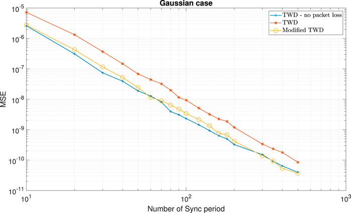
FIGURE 2. Clock skew performance comparison between the modified TWD clock skew estimator (6) with the TWD clock skew estimator (56), for the Gaussian case and the packet loss case (in the Forward path). α =50ppm, Q =5 ms, T_sync =15.6 ms (64 packet/sec), d_ms =0.8 ms, d_sm =1 ms, ${\sigma }_{{\omega }_1}=400\mu s$, ${\sigma }_{{\omega }_2}=10\mu s$. $P_{M_F}=0.9$, $P_{M_R}=0$. The averaged results were obtained for 100 Monte-Carlo trials.

FIGURE 3

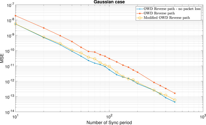
FIGURE 3. Clock skew performance comparison between the modified OWD clock skew estimator for the Reverse path (10) with the OWD clock skew estimator for the Reverse path (58), for the Gaussian case and the packet loss case (in the Forward path). α =50ppm, Q =5 ms, T_sync =15.6 ms (64 packet/sec), d_ms =0.8 ms, d_sm =1 ms, ${\sigma }_{{\omega }_1}=400\mu s$, ${\sigma }_{{\omega }_2}=10\mu s$. $P_{M_F}=0.9$, $P_{M_R}=0$. The averaged results were obtained for 100 Monte-Carlo trials.

FIGURE 4

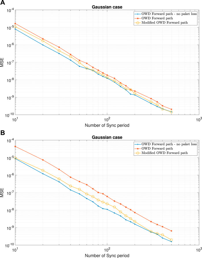
FIGURE 4. Clock skew performance comparison between the modified OWD clock skew estimator for the Forward path (9) with the OWD clock skew estimator for the Forward path (57), for the Gaussian case and the packet loss case (in the Forward path). α =50ppm, Q =5 ms, T_sync =15.6 ms (64 packet/sec), d_ms =0.8 ms, d_sm =1 ms, ${\sigma }_{{\omega }_1}=400\mu s$, ${\sigma }_{{\omega }_2}=10\mu s$. $P_{M_R}=0$. (A) $P_{M_F}=0.9$ (The percentage of missing Sync messages is approx 30%). (B) The percentage of missing Sync messages is 60%. The averaged results were obtained for 100 Monte-Carlo trials.

FIGURE 5

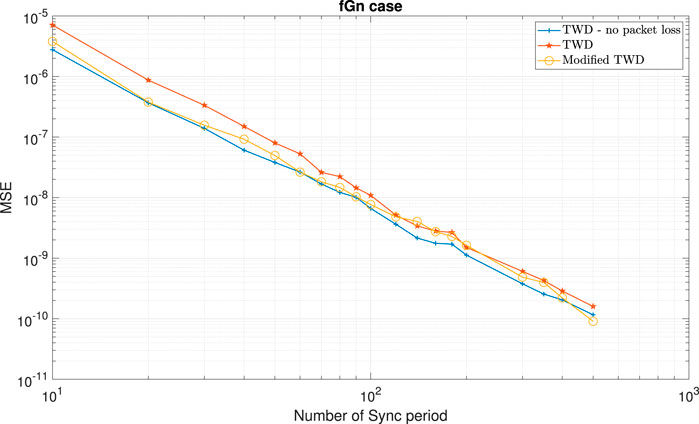
FIGURE 5. Clock skew performance comparison between the modified TWD clock skew estimator (6) with the TWD clock skew estimator (56), for the fGn case and the packet loss case (in the Forward path). α =50ppm, Q =5 ms, T_sync =15.6 ms (64 packet/sec), d_ms =0.8 ms, d_sm =1 ms, ${\sigma }_{{\omega }_1}=400\mu s$, ${\sigma }_{{\omega }_2}=10\mu s$, H_F =0.7, H_R =0.7. $P_{M_F}=0.9$, $P_{M_R}=0$. The averaged results were obtained for 100 Monte-Carlo trials.

FIGURE 6

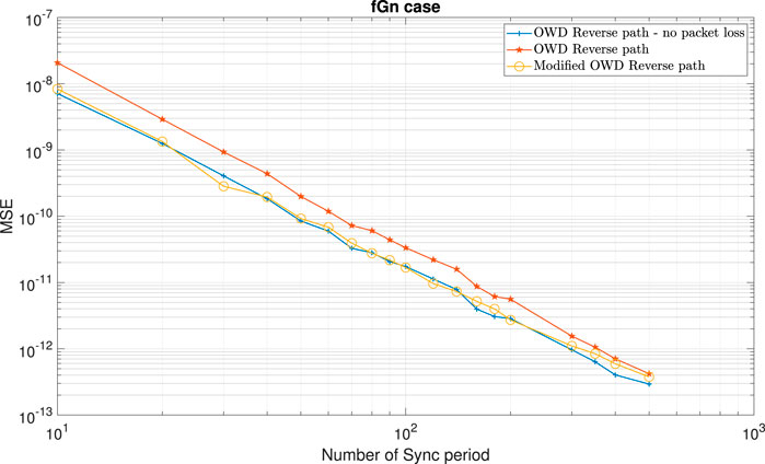
FIGURE 6. Clock skew performance comparison between the modified OWD clock skew estimators for the Reverse path (10) with the OWD clock skew estimator for the Reverse path (58), for the fGn case and the packet loss case (in the Forward path). α =50ppm, Q =5 ms, T_sync =15.6 ms (64 packet/sec), d_ms =0.8 ms, d_sm =1 ms, ${\sigma }_{{\omega }_1}=400\mu s$, ${\sigma }_{{\omega }_2}=10\mu s$, H_F =0.7, H_R =0.7. $P_{M_F}=0.9$, $P_{M_R}=0$. The averaged results were obtained for 100 Monte-Carlo trials.

FIGURE 7

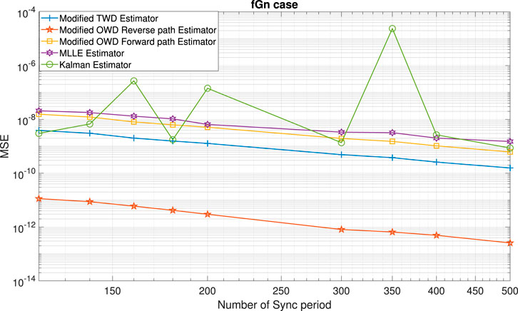
FIGURE 7. Clock skew performance comparison between the modified clock skew estimators ((6); (9); (10)) with the clock skew estimator from Chaloupka et al. [15] denoted here as the Kalman Estimator, and the ML-like clock skew estimator (59) Noh et al. [12] denoted here as MLLE Estimator, for the fGn case and the packet loss case (in the Forward path). α =50ppm, Q =5 ms, T_sync =15.6 ms (64 packet/sec), d_ms =0.8 ms, d_sm =1 ms, ${\sigma }_{{\omega }_1}=400\mu s$, ${\sigma }_{{\omega }_2}=10\mu s$, H_F =0.7, H_R =0.7. $P_{M_F}=0.9$, $P_{M_R}=0$. L =100, Q_KAL =0, δ_σ = δ_μ =1e −4, $\widehat{\mu }[1]=0$. The averaged results were obtained for 100 Monte-Carlo trials.

FIGURE 8

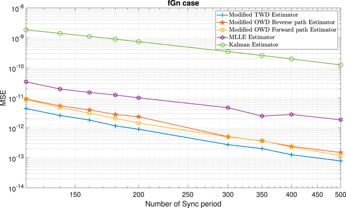
FIGURE 8. Clock skew performance comparison between the modified clock skew estimators ((6); (9); (10)) with the clock skew estimator from [15] denoted here as the Kalman Estimator and the ML-like clock skew estimator from [12] denoted here as MLLE Estimator, for the fGn case and the packet loss case (in the Forward path). α =50ppm, Q =5 ms, T_sync =15.6 ms (64 packet/sec), d_ms =0.8 ms, d_sm =1 ms, ${\sigma }_{{\omega }_1}=10\mu s$, ${\sigma }_{{\omega }_2}=10\mu s$, H_F =0.6, H_R =0.6. $P_{M_F}=0.9$, $P_{M_R}=0$. L =100, Q_KAL =0, δ_σ = δ_μ =1e −4, $\widehat{\mu }[1]=0$. The averaged results were obtained for 100 Monte-Carlo trials.

6.2 The approximated MSE upper bounds

In the following, we test the expressions for the approximated MSE upper bounds ((13); (36); (48)) for various scenarios: 1) Gaussian (H = 0.5) and fGn (H > 0.5) cases. 2) Asymmetry in the PDVs or asymmetry in the Hurst exponent parameters between the Forward and Reverse paths. 3) Randomly distributed missing time stamps or bursts of missing time stamps.Figure 9 and Figure 10 show the performance obtained with the closed-form approximated expressions for the MSE upper bounds ((13), (36), (48)) compared with the simulated performance (MSE) obtained with the modified TWD and OWD clock skew estimators ((6); (9); (10)) with packet loss of 90% in the Forward path. According to Figures 9, 10 the approximated MSE upper bounds ((13); (36); (48)) are very close to the corresponding simulated clock skew performances obtained with (6), (9), and (10). Figure 11 shows the approximated MSE upper bounds ((13); (36); (48)) compared with the simulated performance (MSE) obtained with the modified TWD and OWD clock skew estimators ((6); (9); (10)) for the packet loss case in both paths and asymmetry in the Hurst exponent parameter between the Forward and Reverse path. According to Figure 11, the approximated MSE upper bounds ((13); (36); (48)) are very close to the corresponding simulated clock skew performances obtained with (6), (9) and (10). Until now, we simulated packet loss that was randomly distributed. Next, we tested the performance obtained with the approximated expressions for the upper bounds in case we have a burst of missing messages. Figures 12–14 show the performances of the approximate MSE upper bounds ((13); (36); (48)) compared with the simulated performance (MSE) obtained with the modified TWD and OWD clock skew estimators ((6); (9); (10)) with different lengths of burst for the packet loss case. Figure 12 shows a packet loss burst with the length of 150 Sync periods in the Forward path. In this case, we set r_F = 1 and r_R = 0. Figure 13 shows a packet loss burst with a length of 75 Sync periods in the Forward path. In this case, we set r_F = 0.5 and r_R = 0. In Figure 14, we have a packet loss burst with a length of 75 Sync periods in both paths. In this case, we set r_F = 0.25 and r_R = 0.25 since there is an overlap in the Sync periods of the packet loss burst between the Forward and Reverse paths. According to Figures 12–14, the approximated MSE upper bounds are very close to the corresponding simulated clock skew performances obtained with (6), (9), and (10) before the burst of packet loss begins and after it ends. During the burst mode, the clock skew estimator cannot be updated and thus the clock skew performance (MSE) does not decrease.

FIGURE 9

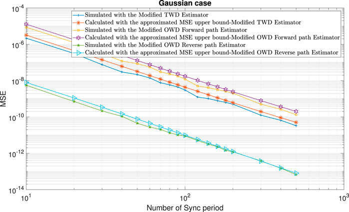
FIGURE 9. Performance comparison between the calculated expressions for the approximated MSE upper bounds ((13); (36); (48)) with the simulated clock skew performance obtained with the modified clock skew estimators ((6); (9); (10)) for the Gaussian case and for the packet loss case (in the Forward path). α =50ppm, Q =5 ms, T_sync =15.6 ms (64 packet/sec), d_ms =0.8 ms, d_sm =1 ms, ${\sigma }_{{\omega }_1}=400\mu s$, ${\sigma }_{{\omega }_2}=10\mu s$, H_F =0.5, H_R =0.5. $P_{M_F}=0.9$, $P_{M_R}=0$, r_F =0, r_R =0. The averaged results were obtained for 100 Monte-Carlo trials.

FIGURE 10

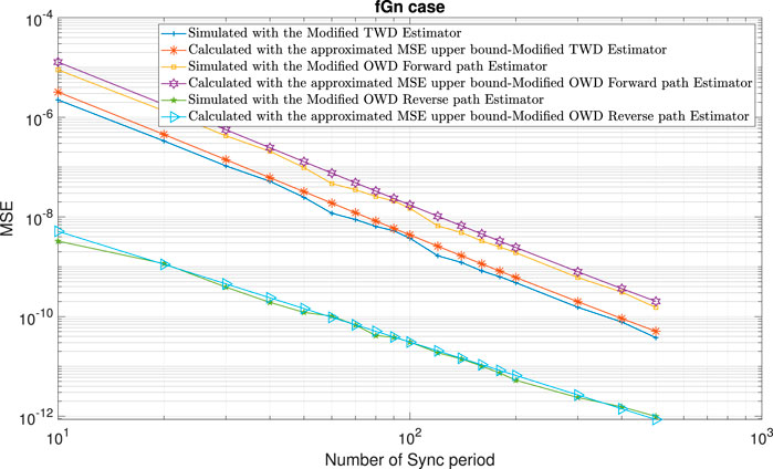
FIGURE 10. Performance comparison between the calculated expressions for the approximated MSE upper bounds ((13); (36); (48)) with the simulated clock skew performance obtained with the modified clock skew estimators ((6); (9); (10)) for the fGn case and for the packet loss case (in the Forward path). α =50ppm, Q =5 ms, T_sync =15.6 ms (64 packet/sec), d_ms =0.8 ms, d_sm =1 ms, ${\sigma }_{{\omega }_1}=400\mu s$, ${\sigma }_{{\omega }_2}=10\mu s$, H_F =0.5, H_R =0.9. $P_{M_F}=0.9$, $P_{M_R}=0$, r_F =0, r_R =0. The averaged results were obtained for 100 Monte-Carlo trials.

FIGURE 11

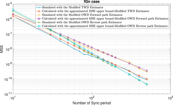
FIGURE 11. Performance comparison between the calculated expressions for the approximated MSE upper bounds ((13); (36); (48)) with the simulated clock skew performance obtained with the modified clock skew estimators ((6); (9); (10)) for the fGn case and for the packet loss case (in the Forward and Reverse paths). α =50ppm, Q =5 ms, T_sync =15.6 ms (64 packet/sec), d_ms =0.8 ms, d_sm =1 ms, ${\sigma }_{{\omega }_1}=200\mu s$, ${\sigma }_{{\omega }_2}=200\mu s$, H_F =0.9, H_R =0.5. $P_{M_F}=0.9$, $P_{M_R}=0.3$, r_F =0, r_R =0. The averaged results were obtained for 100 Monte-Carlo trials.

FIGURE 12

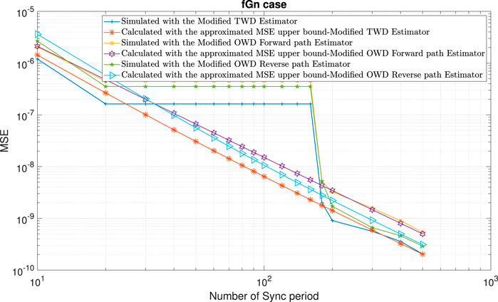
FIGURE 12. Performance comparison between the calculated expressions for the approximated MSE upper bounds ((13); (36); (48)) with the simulated clock skew performance obtained with the modified clock skew estimators ((6); (9); (10)) for the fGn case and the packet loss case (a long burst in the Forward path). α =50ppm, Q =5 ms, T_sync =15.6 ms (64 packet/sec), d_ms =0.8 ms, d_sm =1 ms, ${\sigma }_{{\omega }_1}=200\mu s$, ${\sigma }_{{\omega }_2}=200\mu s$, H_F =0.9, H_R =0.5. $P_{M_F}=0.9$, $P_{M_R}=0$, r_F =1, r_R =0. The averaged results were obtained for 100 Monte-Carlo trials.

FIGURE 13

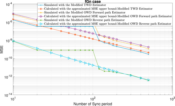
FIGURE 13. Performance comparison between the calculated expressions for the approximated MSE upper bounds ((13); (36); (48)) with the simulated clock skew performance obtained with the modified clock skew estimators ((6); (9); (10)) for the fGn case and for the packet loss case (a sort burst in the Forward path). α =50ppm, Q =5 ms, T_sync =15.6 ms (64 packet/sec), d_ms =0.8 ms, d_sm =1 ms, ${\sigma }_{{\omega }_1}=400\mu s$, ${\sigma }_{{\omega }_2}=10\mu s$, H_F =0.9, H_R =0.5. $P_{M_F}=0.9$, $P_{M_R}=0$, r_F =0.5, r_R =0. The averaged results were obtained for 100 Monte-Carlo trials.

FIGURE 14

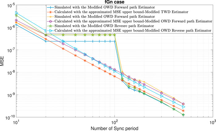
FIGURE 14. Performance comparison between the calculated expressions for the approximated MSE upper bounds ((13); (36); (48)) with the simulated clock skew performance obtained with the modified clock skew estimators ((6); (9); (10)) for the fGn case and the packet loss case (burst in the Forward and Reverse paths). α =50ppm, Q =5 ms, T_sync =15.6 ms (64 packet/sec), d_ms =0.8 ms, d_sm =1 ms, ${\sigma }_{{\omega }_1}=200\mu s$, ${\sigma }_{{\omega }_2}=200\mu s$, H_F =0.9, H_R =0.5. $P_{M_F}=0.9$, $P_{M_R}=0.3$, r_F =0.25, r_R =0.25. The averaged results were obtained for 100Monte-Carlo trials.

7 Conclusion

In this paper, we have derived three modified clock skew estimators (based on the TWD and OWD clock skew estimators from our previous works) applicable in the fGn environment that also answer on the packet loss scenario. These modified clock skew estimators obtain almost the same clock skew performance (MSE) for the packet loss case as those obtained without packet loss. The MSE expression is an essential tool for the system designer in order to estimate the number of Sync periods needed until the clock skew estimator achieves the system’s requirements. In this paper, we derived closed-form approximated expressions for the MSE upper bounds related to the modified TWD and OWD clock skew estimators for the Forward and Reverse paths in the packet loss case. Those closed-form approximated expressions for the MSE upper bounds are suitable for the fGn environment and applicable also if asymmetry in the fixed delays exists or asymmetry in the PDVs is observed or even if asymmetry in the Hurst exponent parameters exists between the Forward and Reverse paths. In addition, those approximated upper bounds are also applicable for cases where the missing time stamps are not randomly distributed over time but come in burst mode. Simulation results confirm that the approximated MSE upper bounds are very tight to the corresponding simulated clock skew performances obtained with our modified clock skew estimators in this work. In the future, we would like to benchmark the modified clock skew estimators against the MLLE and Kalman ones on real-life data sets instead of only simulated ones.

Data availability statement

The original contributions presented in the study are included in the article/Supplementary material, further inquiries can be directed to the corresponding author.

Author contributions

All authors listed have made a substantial, direct, and intellectual contribution to the work and approved it for publication.

Conflict of interest

The authors declare that the research was conducted in the absence of any commercial or financial relationships that could be construed as a potential conflict of interest.

Publisher’s note

All claims expressed in this article are solely those of the authors and do not necessarily represent those of their affiliated organizations, or those of the publisher, the editors and the reviewers. Any product that may be evaluated in this article, or claim that may be made by its manufacturer, is not guaranteed or endorsed by the publisher.

References

1. Arnold D. IEEE 1588-2019 - IEEE standard for a precision clock synchronization protocol for networked measurement and control systems. IEEE (2019).

Google Scholar

2. Avraham Y, Pinchas M. A novel clock skew estimator and its performance for the IEEE 1588v2 (PTP) case in fractional Gaussian noise/generalized fractional Gaussian noise environment. Front Phys (2021) 9:1–21. doi:10.3389/fphy.2021.796811

CrossRef Full Text | Google Scholar

3. Avraham Y, Pinchas M. Two novel one-way delay clock skew estimators and their performances for the fractional Gaussian noise/generalized fractional Gaussian noise environment applicable for the IEEE 1588v2 (PTP) case. Front Phys (2022) 10:1–19. doi:10.3389/fphy.2022.867861

CrossRef Full Text | Google Scholar

4. Karthik AK, Blum RS. Robust phase offset estimation for IEEE 1588 PTP in electrical grid networks. In: 2018 IEEE Power and Energy Society General Meeting; 05-10 August 2018; Portland, OR, USA (2018). doi:10.1109/PESGM.2018.8586488

CrossRef Full Text | Google Scholar

5. Karthik AK, Blum RS. Optimum full information, unlimited complexity, invariant, and minimax clock skew and offset estimators for IEEE 1588. IEEE Trans Commun (2019) 67:3624–37. doi:10.1109/TCOMM.2019.2900317

CrossRef Full Text | Google Scholar

6. Karthik AK, Blum RS. Robust clock skew and offset estimation for IEEE 1588 in the presence of unexpected deterministic path delay asymmetries. IEEE Trans Commun (2020) 68:5102–19. doi:10.1109/TCOMM.2020.2991212

CrossRef Full Text | Google Scholar

7. Satheesh Kumar S, Kemparaj P. Enhanced algorithms for clock selection in a packet based synchronization method. In: 2019 IEEE 9th Symposium on Computer Applications and Industrial Electronics (ISCAIE); 27-28 April 2019; Malaysia (2019). doi:10.1109/ISCAIE.2019.8743747

CrossRef Full Text | Google Scholar

8. Li M. Multi-fractal traffic and anomaly detection in computer communications. 1 edn. Boca Raton: CRC Press (2022). doi:10.1201/9781003268802

CrossRef Full Text | Google Scholar

9. Li M. Fractal teletraffic modeling and delay bounds in computer communications. 1 edn. Boca Raton: CRC Press (2022). doi:10.1201/9781003354987

CrossRef Full Text | Google Scholar

10. Puttnies H, Danielisx P, Timmermann D. PTP-LP: Using linear programming to increase the delay robustness of IEEE 1588 PTP. In: IEEE Global Communications Conference; 09-13 December 2018; Abu Dhabi, United Arab Emirates (2018). doi:10.1109/GLOCOM.2018.8647777

CrossRef Full Text | Google Scholar

11. Li J, Jeske DR. Maximum likelihood estimators of clock offset and skew under exponential delays. Appl Stochastic Models Business Industry (2009) 25:445–59. doi:10.1002/asmb.777

CrossRef Full Text | Google Scholar

12. Noh KL, Chaudhari QM, Serpedin E, Suter BW. Novel clock phase offset and skew estimation using two-way timing message exchanges for wireless sensor networks. IEEE Trans Commun (2007) 55:766–77. doi:10.1109/TCOMM.2007.894102

CrossRef Full Text | Google Scholar

13. Giorgi G, Narduzzi C. Performance analysis of Kalman-filter-based clock synchronization in IEEE 1588 networks. IEEE Trans Instrumentation Meas (2011) 60:2902–9. doi:10.1109/TIM.2011.2113120

CrossRef Full Text | Google Scholar

14. Avraham Y, Pinchas M. PTP clock skew estimator performance with packet impairments. In: SEEEI Electricity & Energy 2022; 01 Nov 2022; Eilat, Israel (2022).

Google Scholar

15. Chaloupka Z, Alsindi N, Aweya J. Clock skew estimation using Kalman filter and IEEE 1588v2 PTP for telecom networks. IEEE Commun Lett (2015) 19:1181–4. doi:10.1109/LCOMM.2015.2427158

CrossRef Full Text | Google Scholar

16. Li M, Zhao W. On bandlimitedness and lag-limitedness of fractional Gaussian noise. Physica A (2013) 392:1955–61. doi:10.1016/j.physa.2012.12.035

CrossRef Full Text | Google Scholar

17. Li M. Generalized fractional Gaussian noise and its application to traffic modeling. Physica A: Stat Mech its Appl (2021) 579:126138. doi:10.1016/j.physa.2021.126138

CrossRef Full Text | Google Scholar

Appendix A

In the following, we present the proof of Theorem 1 from Section 4.

Based on (1) and (2) we can write:

$T_{1,j}\left(i\right)+{\bar{\mathrm{\Omega }}}_{1,j}\left(i\right)=\left(1+{\alpha }_{j,i}\right){\widehat{T}}_{2,j}\left(i\right)(\mathrm{A1})$

And

${\widehat{T}}_{4,j}\left(i\right)-{\bar{\mathrm{\Omega }}}_{2,j}\left(i\right)=\left(1+{\alpha }_{j,i}\right)T_{3,j}\left(i\right)(\mathrm{A2})$

where ${\bar{\mathrm{\Omega }}}_{n,j}(i)$ for n = 1, 2 is the subtraction of two unknown PDV variables from different Sync periods and is defined as:

${\bar{\mathrm{\Omega }}}_{n,j}\left(i\right)={\bar{\omega }}_n\left[j+i\right]-{\bar{\omega }}_n\left[j\right](\mathrm{A3})$

Please note that unlike in [2] and [3], we cover here also the case where packets may get lost and those missing time stamps are estimated in this work based on (3) and (4). Thus, when $T_{\tilde{l},j}(i)$ can be derived via the received time stamps (without the need for any estimation), we may write: ${\widehat{T}}_{\tilde{l},j}(i)=T_{\tilde{l},j}(i)$, ${\bar{\omega }}_n[j+1]={\omega }_n[j+1]$ and ${\bar{\omega }}_n[j]={\omega }_n[j]$, where ω_n [j] and ${\bar{\omega }}_n[j]$ are the unknown PDV variables related to the received time stamps and the estimated time stamps, respectively. Otherwise, we apply the estimated time stamps ${\widehat{t}}_{\tilde{l}}[j]$ or ${\widehat{t}}_{\tilde{l}}[j+i]$ to derive ${\widehat{T}}_{\tilde{l},j}(i)$, and use ${\bar{\omega }}_n[j]$ in our calculations. Based on Eqs. A1, A2 we can write:

${\alpha }_{\begin{array}{c}i,j\end{array}}=\frac{1}{2}\left(\left(\frac{T_{1,j}\left(i\right)}{{\widehat{T}}_{2,j}\left(i\right)}+\frac{T_{4,j}\left(i\right)}{{\widehat{T}}_{3,j}\left(i\right)}\right)+\left(\frac{{\bar{\mathrm{\Omega }}}_{1,j}\left(i\right)}{T_{2,j}\left(i\right)}-\frac{{\bar{\mathrm{\Omega }}}_{2,j}\left(i\right)}{T_{3,j}\left(i\right)}\right)\right)-1(\mathrm{A4})$

From [2] we have:

$\alpha =\frac{2}{J\left(J-1\right)}{\displaystyle \sum _{i=1}^{J-1}}{\displaystyle \sum _{j=1}^{J-i}}{\alpha }_{j,i}(\mathrm{A5})$

By putting Eq. A4 into Eq. A5, we may write:

$\begin{array}{cc}\hfill \alpha & =\frac{1}{J\left(J-1\right)}\left({\displaystyle \sum _{i=1}^{J-1}}{\displaystyle \sum _{j=1}^{J-i}}\left(\frac{T_{1,j}\left(i\right)}{{\widehat{T}}_{2,j}\left(i\right)}+\frac{{\widehat{T}}_{4,j}\left(i\right)}{T_{3,j}\left(i\right)}\right)-1+{\displaystyle \sum _{i=1}^{J-1}}{\displaystyle \sum _{j=1}^{J-i}}\left(\frac{{\bar{\mathrm{\Omega }}}_{1,j}\left(i\right)}{{\widehat{T}}_{2,j}\left(i\right)}-\frac{{\bar{\mathrm{\Omega }}}_{2,j}\left(i\right)}{T_{3,j}\left(i\right)}\right)\right)\hfill \\ \hfill & =\widehat{\alpha }+\frac{1}{J\left(J-1\right)}{\displaystyle \sum _{i=1}^{J-1}}{\displaystyle \sum _{j=1}^{J-i}}\left(\frac{{\bar{\mathrm{\Omega }}}_{1,j}\left(i\right)}{{\widehat{T}}_{2,j}\left(i\right)}-\frac{{\bar{\mathrm{\Omega }}}_{2,j}\left(i\right)}{T_{3,j}\left(i\right)}\right)=\widehat{\alpha }+e\hfill \end{array}(\mathrm{A6})$

where e is its error.

Based on Eqs. A1, A2, and [3], we can write the modified OWD clock skew estimators for the Forward and Reverse paths. The modified OWD clock skew estimator for the Forward path is:

$\begin{array}{cc}\hfill {\alpha }_F& =\frac{2}{J\left(J-1\right)}\left({\displaystyle \sum _{i=1}^{J-1}}{\displaystyle \sum _{j=1}^{J-i}}\left(\frac{T_{1,j}\left(i\right)}{{\widehat{T}}_{2,j}\left(i\right)}\right)-1+{\displaystyle \sum _{i=1}^{J-1}}{\displaystyle \sum _{j=1}^{J-i}}\left(\frac{{\bar{\mathrm{\Omega }}}_{1,j}\left(i\right)}{{\widehat{T}}_{2,j}\left(i\right)}\right)\right)\hfill \\ \hfill & ={\widehat{\alpha }}_F+\frac{2}{J\left(J-1\right)}{\displaystyle \sum _{i=1}^{J-1}}{\displaystyle \sum _{j=1}^{J-i}}\left(\frac{{\bar{\mathrm{\Omega }}}_{1,j}\left(i\right)}{{\widehat{T}}_{2,j}\left(i\right)}\right)={\widehat{\alpha }}_F+e_F\hfill \end{array}(\mathrm{A7})$

And the modified OWD clock skew estimator for the Reverse path is:

$\begin{array}{cc}\hfill {\alpha }_R& =\frac{2}{J\left(J-1\right)}\left({\displaystyle \sum _{i=1}^{J-1}}{\displaystyle \sum _{j=1}^{J-i}}\left(\frac{{\widehat{T}}_{4,j}\left(i\right)}{T_{3,j}\left(i\right)}\right)-1-{\displaystyle \sum _{i=1}^{J-1}}{\displaystyle \sum _{j=1}^{J-i}}\left(\frac{{\bar{\mathrm{\Omega }}}_{2,j}\left(i\right)}{T_{3,j}\left(i\right)}\right)\right)\hfill \\ \hfill & ={\widehat{\alpha }}_R-\frac{2}{J\left(J-1\right)}{\displaystyle \sum _{i=1}^{J-1}}{\displaystyle \sum _{j=1}^{J-i}}\left(\frac{{\bar{\mathrm{\Omega }}}_{2,j}\left(i\right)}{T_{3,j}\left(i\right)}\right)={\widehat{\alpha }}_R-e_R\hfill \end{array}(\mathrm{A8})$

where e_F and e_R are the errors of the modified OWD clock skew estimators for the Forward and Reverse paths, respectively. This completes our proof.