Physically significant solitary wave solutions to the space-time fractional Landau–Ginsburg–Higgs equation via three consistent methods

The Landau–Ginzburg–Higgs equation (LGHE) is a mathematical model used to describe nonlinear waves that exhibit weak scattering and long-range connections in the tropical and mid-latitude troposphere as interactions between equatorial and mid-latitude Rossby waves. This study assessed the fractional Landau–Ginzburg–Higgs model, previously introduced in truncated M-fractional derivatives utilizing the $\left(G^{\prime }/G,1/G\right)$, modified $\left(G^{\prime }/G^2\right)$, and new auxiliary equation methods. Using these techniques, different solutions, including unknown parameters, were obtained in trigonometric, hyperbolic, and exponential functions. This study investigated how varying values of the fractional parameter affected the deeds of the solutions obtained for the given conditions. The predicted solutions, obtained under restricted conditions, were visualized through 2D, 3D, and contour plots using appropriate parameter values. The attained results were confirmed for the aforementioned equations using symbolic soft computations. Moreover, the outcomes confirmed that the methods used in this study were effective mathematical tools for discovering exact solitary wave solutions to nonlinear models encountered in various areas of science and engineering.

1 Introduction

Non-linear partial differential equations (NLPDEs) play significant roles in physics, mathematical engineering, and other phenomena such as heat flow, plasma physics, wave propagation, shallow water waves, chemically dispersed electricity, quantum mechanics, fluid dynamics, and reactive materials. NLPDEs also play substantial roles in nonlinear optical fibers and quantum fields, such as nonlinear wave equations, Monge–Ampere equations, Burgers equations, Liouville equations, Fisher equations, and Kolmogorov–Petrovskii–Piskunov equations [1–4]. These equations assist in the implementation of essential parts of the soliton solution. The soliton is stimulated during diffusion by eliminating the effects of diffusion. Now, soliton assessment is very common [5]. Solitons are solutions to large, weakly detached partial differential equations (PDEs) for physical structures. Nowadays, many models are considered for computing the soliton solutions (SS) [6–8]. Among these, the Landau–Ginzburg–Higgs (LGH) model [9, 10] is one of the most considered in recent years, as follows:

$\frac{{\partial }^{2}v}{\partial t^2}-\frac{{\partial }^{2}v}{\partial x^2}-g^{2}v+h^2{v}^3=0,(1)$

where $v=v\left(x,t\right)$ is the ion-cyclotron wave electrostatic potential $g$ and $h$ are real parameters and $x,t$ indicate the nonlinearized spatial and temporal coordinates. Lev Davidovich Landau and Vitaly Lazarevich Ginzburg designed the LGHE (1) to describe superconductivity and drift cyclotron waves in radially inhomogeneous plasmas of integrated ion cyclotrons [11]. Numerous methods have been used to determine the distinctive SS of the integrable nonlinear evolution equation (NLEE) (1). Bekir and Unsal [12] provided exponential function solutions by using the first integral method for NLEE (1). Iftikhar et al. [13] utilized the $\left(G^{\prime }/G,1/G\right)$-expansion method and inspected a variety of analytical solutions for NLEE (1). They also determined general and kinked shape soliton solutions for different parameter selections. Barman et al. [14, 15] obtained various analytical solutions using the Kudryashov technique comprising the undisclosed parameters of Eq. 1. In addition, they employed the tanh function to create solutions with soliton-like shapes, such as dark solitons, bright solitons, peakons, compactons, and periodic solutions, among others. These solutions can be utilized to investigate the propagation of various waves, such as tidal and tsunami waves, ion-acoustic waves, and magneto-sound waves in plasma. Islam and Akbar [16] used the IBSEF and presented innumerable stable solutions. The results provided several soliton shapes, which considered one-way wave propagation with diffuse systems in nonlinear science.

For two centuries, fractional calculus has fascinated many intellectuals’ curiosity. Use them to develop many nonlinear aspects, inclosing bioprocesses, chemical processes, fluid mechanics, etc. In the traditional integer order, the fractional-order PDEs are used to generalize PDEs. Several definitions of the fractional derivative exist in the literature, such as Riemann–Liouville [17], Caputo [18], Caputo–Fabrizio [19], conformable fractional derivative (FD) [20], and beta-derivative [21] to solve non-integer-order models. Studies have shown that these definitions of FD do not meet some of the basic assets of derivatives, such as product and chain rules. Sousa and Oliveira [22] developed a novel truncated-M fractional derivative that meets numerous properties considered to be the FD’ boundary. This derivative has interesting results in different areas, such as chaos theory, biological modeling, circuit analysis, optical physics, and disease analysis.

The core aim of this study was to explore the space-time fractional LGH model [23], symbolized as

$D_{M,t}^{2\alpha ,\beta }v-D_{M,x}^{2\alpha ,\beta }v-g^{2}v+h^2{v}^3=0,0<\alpha <1,\beta >0,(2)$

where $\alpha$ and $\beta$ are the fractional parameters representing the fractional time derivative’s order.

The fundamental consideration of this exploration was to take advantage of the novel indication of fractional-order derivatives, called truncated truncated-M fractional derivatives [22, 24, 25], for space-time fractional LGHE [23], and to use the $\left(G^{\prime }/G,1/G\right),$ modified $\left(G^{\prime }/G^2\right)$, and new auxiliary equation methods (NAEMs) [23, 26, 27] to obtain new inclusive solitary solutions in the form of solutions of bright, dark, single solitons, and periodic isolated waves. Up to now, the results have different corporate and diverse forms, which have not been reported previously [23].

Moreover, the planned technique has been used to solve various models. For instance, Hafiz [28] employed the $\left(G^{\prime }/G,1/G\right)$-expansion method to determine the closed-form solutions of the generalized fractional reaction Duffing model and the density-dependent fractional diffusion-reaction equation. Li et al. [29] discovered the traveling wave solutions of the Zakharov equation, and Zayed et al. [30] established solutions to the nonlinear Kdv–mKdv equation. Uddin [31] and Wazwaz [32] provided general solutions for the fifth-order NLEEs and the Burger KP-equation, respectively. Sirisubtawee [33] found exact traveling wave solutions for nonlinear fractional evolution equations. Traveling wave solutions for the nonlinear Schrodinger equation with third-order dispersion were obtained using the modified $\left(G^{\prime }/G^2\right)$-expansion model [34]. The Fokas–Lenells equations were solved using this technique to regulate different traveling wave solutions [35]. Aljahdaly [36] extended the NLEEs and described the general exact traveling wave solutions. Dragon and Donmez [37] discovered solutions in the form of traveling waves for the Gardner equation and then used these solutions to address different plasma-related issues. The Sharma–Tasso–Olver (STO) equations were also solved, and exact nonlinear and super nonlinear traveling wave solutions were obtained [38]. Jhangeer et al. [39] used the new auxiliary equations method to find innovative soliton solutions for the fractional Caudrey–Dodd–Gibbon–Sawada–Kotera equation. Raza et al. [40] obtained the new optical solitary wave solitons of the three-dimensional Fractional Wazwaz–Benjamin–Bona–Mahony (WBBM) equation. Furthermore, Riaz et al. [41] scrutinized the various forms of solitary wave solutions for the modified equal-width wave equation.

This work is structured into six sections. Section 2 presents the truncated M-fractional derivative and its properties, which is the foundation of the proposed methods. The methodologies of the three proposed approaches are discussed in Section 3, where we explain how to use the truncated M-fractional derivative to solve mathematical models. Section 4 involves a mathematical examination of the models we have presented and the solutions we have obtained using the proposed methods. We compare them with existing methods in the literature. Section 5 provides a graphical representation of the obtained solutions for each analyzed model. Finally, Section 6 provides the study conclusion by summarizing the key findings and their implications.

2 Truncated M-fractional derivative and its properties

The following section will discuss the truncated M-fractional derivative (TMFD) of order $\alpha$ with its properties.

Definition 2.1. Let $f:\left(0,\infty \right)\to R,$ then, the TMFD of a function $f$ of order $\alpha$ is determined as

$D_M^{\alpha ,\beta }f\left(t\right)={\lim }_{\epsilon \to 0}\frac{f\left(t{\in }_{\beta }\left(\epsilon t^{1-\alpha }\right)\right)-f\left(t\right)}{\epsilon },\mathrm{f}\mathrm{o}\mathrm{r}\mathrm{a}\mathrm{l}\mathrm{l}t>0,0<\alpha <1,\beta >0,$

where $\alpha {\in }_{\beta }\left(\cdot \right)$ is a truncated Mittag–Leffler function of one parameter [22].

Properties 2.2. Let $\alpha \in \left.\left(0,1\right.\right],\beta >0$ and $f=f\left(t\right),g=g\left(t\right)$ be $\alpha$-differentiable at a point $t>0,$ then:

1. $D_M^{\alpha ,\beta }\left(af+bg\right)=a{D}_M^{\alpha ,\beta }f+b{D}_M^{\alpha ,\beta }g,$ $\forall$ $a,b\in R.$

2. $D_M^{\alpha ,\beta }\left(c\right)=0,\mathrm{w}\mathrm{h}\mathrm{e}\mathrm{r}\mathrm{e}f\left(t\right)=c,\mathrm{i}\mathrm{s}\mathrm{a}\mathrm{c}\mathrm{o}\mathrm{n}\mathrm{s}\mathrm{t}\mathrm{a}\mathrm{n}\mathrm{t}.$

3. $D_M^{\alpha ,\beta }\left(f\cdot g\right)=D_M^{\alpha ,\beta }f+D_M^{\alpha ,\beta }g.$

4. $D_M^{\alpha ,\beta }\left(\frac{f}{g}\right)=\frac{g{D}_M^{\alpha ,\beta }f-f{D}_M^{\alpha ,\beta }g}{g^2}.$

5. If $f$ is differentiable, then

$D_M^{\alpha ,\beta }f\left(t\right)=\frac{t^{1-\alpha }}{\mathrm{\Gamma }\left(\beta +1\right)}\frac{df}{dt}.(3)$

6. $D_M^{\alpha ,\beta }\left(f\circ g\right)\left(t\right)=f^{\prime }\left(g\left(t\right)\right)D_M^{\alpha ,\beta }g\left(t\right),\mathrm{f}\mathrm{o}\mathrm{r}f\mathrm{d}\mathrm{i}\mathrm{f}\mathrm{f}\mathrm{e}\mathrm{r}\mathrm{e}\mathrm{n}\mathrm{t}\mathrm{i}\mathrm{a}\mathrm{b}\mathrm{l}\mathrm{e}\mathrm{a}\mathrm{t}g\left(t\right).$

3 General form of the methods

3.1 $\left(G^{\prime }/G,1/G\right)$-expansion method

The core steps of the $\left(G^{\prime }/G,1/G\right)$-expansion model [24, 28] for discovering traveling wave solutions to nonlinear evolution equations are outlined in this section. We begin by examining the second-order linear ordinary differential equation (ODE):

$G^{″}\left(\eta \right)+\lambda G\left(\eta \right)=\mu ,(4)$

where $\varphi =\raisebox{1ex}{$G^{\prime }$}\!\left/ \!\raisebox{-1ex}{$G$}\right.\mathrm{a}\mathrm{n}\mathrm{d}\psi =\raisebox{1ex}{$1$}\!\left/ \!\raisebox{-1ex}{$G$}\right.,$ then

$\varphi ´=-{\varphi }^2+\mu \psi -\lambda ,\psi ´=-\varphi \psi .(5)$

Case 1:. When $\lambda <0,$ the general solutions of Eq. 4 is given as

$G\left(\eta \right)=A_1\sinh \left(\sqrt{-\lambda }\eta \right)+A_2\cosh \left(\sqrt{-\lambda }\eta \right)+\frac{\mu }{\lambda },(6)$

and we have

${\psi }^2=\frac{-\lambda }{{\lambda }^2\sigma +{\mu }^2}\left({\varphi }^2-2\mu \psi +\lambda \right),(7)$

where $A_1\mathrm{a}\mathrm{n}\mathrm{d}{A}_2$ are arbitrary integration constants and $\sigma ={A_1}^2-{A_2}^2.$

Case 2:. When $\lambda >0,$ the general solution of Eq. 4 is clearly

$G\left(\eta \right)=A_1\sin \left(\sqrt{\lambda }\eta \right)+A_2\cos \left(\sqrt{\lambda }\eta \right)+\frac{\mu }{\lambda },(8)$

and we have

${\psi }^2=\frac{\lambda }{{\lambda }^2\sigma -{\mu }^2}\left({\varphi }^2-2\mu \psi +\lambda \right),(9)$

where $A_1\mathrm{a}\mathrm{n}\mathrm{d}{A}_2$ are arbitrary integration constants and $\sigma ={A_1}^2+{A_2}^2.$

Case 3:. When $\lambda =0,$ the general solutions of Eq. 4 is

$G\left(\eta \right)=\frac{\mu }{2}{\eta }^2+A_1\eta +A_2,(10)$

and we have

${\psi }^2=\frac{1}{{A_1}^2-2\mu A_2}\left({\varphi }^2-2\mu \psi \right),(11)$

where $A_1\mathrm{a}\mathrm{n}\mathrm{d}{A}_2$ are arbitrary integration constants.Consider the NLPDE, such as

$Q\left(u,u_t,u_x,u_{tt},u_{xt},u_{xx},\dots \right)=0.(12)$

The unfamiliar function $u=u\left(x,t\right)$ is represented by a $Q$ polynomial of the variable and its partial derivatives. The key phases involved in the $\left(G^{\prime }/G,1/G\right)$-expansion model are as follows:

Step 1:. By coordinate transformation

$\eta =x-ct,u\left(x,t\right)=v\left(\eta \right).(13)$

where $c$ is the speed of the traveling wave.The wave variable allows us to reduce Eq. 12 into a nonlinear ODE for $v=v\left(\eta \right):$

$R\left(v,v^{\prime },v^{″},v‴,...\right)=0,(14)$

where $R$ is a polynomial of $v\left(\eta \right)$ and its total derivatives concerning $\eta .$

Step 2:. Assume that a polynomial can express the solutions of Eq. 14 in two variables $\varphi$ and $\psi$ as

$v\left(\eta \right)={\displaystyle \sum _{i=0}^m}{a}_i{\varphi }^i+{\displaystyle \sum _{i=0}^m}{b}_i{\varphi }^{i-1}\psi .(15)$

To determine the values of the constants $a_i\left(i=0,1,\dots ,m\right)\mathrm{a}\mathrm{n}\mathrm{d}{b}_i\left(i=1,\dots ,m\right)$ and the positive integer $m$, a homogenous imbalance is used among the highest-order derivatives and the nonlinear terms in the given ODE Eq. 14.

Step 3:. Substitute Eq. 15 into Eq. 14 along with Eqs 5 and 7, reducing the left-hand side of the ODE into a polynomial in terms of $\varphi$ and $\psi$, with a maximum degree of 1 for $\psi$. A system of algebraic equations is obtained by setting each coefficient of the polynomial to zero, which can be solved with the aid of Mathematica software to obtain the values for $a_i\left(i=0,1,\dots ,m\right),b_i\left(i=1,\dots ,m\right),c,\mu ,\lambda \left(\lambda <0\right),A_1\mathrm{a}\mathrm{n}\mathrm{d}{A}_2.$

Step 4:. Substitute the values obtained for a_i (i = 0, 1, …, m), b_i (i = 1, …, m), c, μ, λ(λ<0), A₁ and A₂ in Eq. 15 to determine the traveling wave solutions in terms of hyperbolic functions, as expressed in Eq. 14.

Step 5:. Similarly, substitute Eq. 15 into Eq. 14 along with Eq. 5 and either Eq. 9 or Eq. 11 to obtain exact traveling wave solutions expressed in terms of trigonometric or rational functions, respectively.

3.2 The modified $\left(G^{\prime }/G^2\right)$-expansion method

We outline the fundamental steps of the modified $\left(G^{\prime }/G^2\right)$-expansion method [24, 29] as follows:

Step 1:. Start by considering Eqs 12–14.

Step 2:. Extend the solutions to Eq. 14 as follows:

$v\left(\eta \right)={\displaystyle \sum _{i=0}^m}{a}_i{\left(\frac{G^{\prime }}{G^2}\right)}^i,(16)$

where $a_i\left(i=\mathrm{0,1,2,3},\dots ,m\right)$ are constants and found later. It is important that $a_i\ne 0.$The function $G=G\left(\eta \right)$ satisfies the following Riccati equation:

${\left(\frac{G^{\prime }}{G^2}\right)}^{\prime }={\lambda }_1{\left(\frac{G^{\prime }}{G^2}\right)}^2+{\lambda }_0,(17)$

where ${\lambda }_0$ and ${\lambda }_1$ are constants.We can obtain the following solutions to Eq. 17 under different conditions ${\lambda }_0$:When ${\lambda }_0{\lambda }_1<0,$

$\left(\frac{G^{\prime }}{G^2}\right)=-\frac{\sqrt{\left|{\lambda }_0{\lambda }_1\right|}}{{\lambda }_1}+\frac{\sqrt{\left|{\lambda }_0{\lambda }_1\right|}}{2}\left[\frac{C_1\sinh \left(\sqrt{{\lambda }_0{\lambda }_1}\eta \right)+C_2\cosh \left(\sqrt{{\lambda }_0{\lambda }_1}\eta \right)}{C_1\cosh \left(\sqrt{{\lambda }_0{\lambda }_1}\eta \right)+C_2\sinh \left(\sqrt{{\lambda }_0{\lambda }_1}\eta \right)}\right].(18)$

When ${\lambda }_0{\lambda }_1>0,$

$\left(\frac{G^{\prime }}{G^2}\right)=\sqrt{\frac{{\lambda }_0}{{\lambda }_1}}\left[\frac{C_1\cos \left(\sqrt{{\lambda }_0{\lambda }_1}\eta \right)+C_2\sin \left(\sqrt{{\lambda }_0{\lambda }_1}\eta \right)}{C_1\sin \left(\sqrt{{\lambda }_0{\lambda }_1}\eta \right)-C_2\sin \left(\sqrt{{\lambda }_0{\lambda }_1}\eta \right)}\right].(19)$

When ${\lambda }_0=0$ and ${\lambda }_1\ne 0,$

$\left(\frac{G^{\prime }}{G^2}\right)=-\frac{C_1}{{\lambda }_1\left(C_1\eta +C_2\right)},(20)$

where $C_1$ and $C_2$ are arbitrary constants.

Step 3:. If we substitute Eq. 16 and Eq. 17 into Eq. 14 and equate the coefficients of each power of ${\left(\frac{G^{\prime }}{G^2}\right)}^i$ to zero, a set of algebraic equations can be obtained. These equations can then be solved to determine the values of $a_i,{\lambda }_0,{\lambda }_1,c$, and other parameters.

Step 4:. Replacing Eq. 16 of which ${\alpha }_i,c$, and other parameters are found in step 3 in Eq. 13, we obtain the solutions for Eq. 12.

3.3 The new auxiliary equation method

Now, we will designate the elementary steps of the new auxiliary equation method [39, 40].

Step 1:. Consider Eqs 12–14.

Step 2:. Subsequently determine the solutions of Eq. 14:

$v\left(\eta \right)={\displaystyle \sum _{i=0}^m}{a}_i{\gamma }^{if\left(\eta \right)},(21)$

which satisfies the auxiliary equation:

$f^{\prime }\left(\eta \right)=\frac{1}{\ln \left(\gamma \right)}\left(\mu {\gamma }^{-f\left(\eta \right)}+\lambda +\zeta {\gamma }^{f\left(\eta \right)}\right),(22)$

where $a_0,a_1,a_2,\dots ,a_m$ are coefficients to be solved such that $a_m\ne 0.$ We then utilized the balancing principle to obtain the value of $m,$ which states that we can find $m$ by equating the nonlinear term of Eq. 14 with the highest-order derivative.For Eq. 22, the family of solutions can be attained as follows:Family-1 When ${\lambda }^2-4\mu \zeta <0$ and $\zeta \ne 0,$

$\begin{array}{l}{\gamma }^{f\left(\eta \right)}=\frac{-\lambda }{2\zeta }+\frac{\sqrt{4\mu \zeta -{\lambda }^2}}{2\zeta }\tan \left(\frac{\sqrt{4\mu \zeta -{\lambda }^2}}{2}\eta \right),\\ {\gamma }^{f\left(\eta \right)}=\frac{-\lambda }{2\zeta }-\frac{\sqrt{4\mu \zeta -{\lambda }^2}}{2\zeta }\cot \left(\frac{\sqrt{4\mu \zeta -{\lambda }^2}}{2}\eta \right).\end{array}$

Family-2 When ${\lambda }^2-4\mu \zeta >0$ and $\zeta \ne 0,$

$\begin{array}{l}{\gamma }^{f\left(\eta \right)}=\frac{-\lambda }{2\zeta }-\frac{\sqrt{{\lambda }^2-4\mu \zeta }}{2\zeta }\tanh \left(\frac{\sqrt{{\lambda }^2-4\mu \zeta }}{2}\eta \right),\\ {\gamma }^{f\left(\eta \right)}=\frac{-\lambda }{2\zeta }-\frac{\sqrt{{\lambda }^2-4\mu \zeta }}{2\zeta }\coth \left(\frac{\sqrt{{\lambda }^2-4\mu \zeta }}{2}\eta \right).\end{array}$

Family-3 When ${\lambda }^2+4{\mu }^2<0,\zeta \ne 0$ and $\zeta =-\mu ,$

$\begin{array}{l}{\gamma }^{f\left(\eta \right)}=\frac{\lambda }{2\mu }-\frac{\sqrt{-4{\mu }^2-{\lambda }^2}}{2\mu }\tan \left(\frac{\sqrt{-4{\mu }^2-{\lambda }^2}}{2}\eta \right),\\ {\gamma }^{f\left(\eta \right)}=\frac{\lambda }{2\mu }+\frac{\sqrt{-4{\mu }^2-{\lambda }^2}}{2\mu }\cot \left(\frac{\sqrt{-4{\mu }^2-{\lambda }^2}}{2}\eta \right).\end{array}$

Family-4 When ${\lambda }^2+4{\mu }^2>0,\zeta \ne 0$ and $\zeta =-\mu ,$

$\begin{array}{l}{\gamma }^{f\left(\eta \right)}=\frac{\lambda }{2\mu }+\frac{\sqrt{4{\mu }^2+{\lambda }^2}}{2\mu }\tanh \left(\frac{\sqrt{4{\mu }^2+{\lambda }^2}}{2}\eta \right),\\ {\gamma }^{f\left(\eta \right)}=\frac{\lambda }{2\mu }+\frac{\sqrt{4{\mu }^2+{\lambda }^2}}{2\mu }\coth \left(\frac{\sqrt{4{\mu }^2+{\lambda }^2}}{2}\eta \right).\end{array}$

Family-5 When ${\lambda }^2-4{\mu }^2<0$ and $\zeta =\mu ,$

$\begin{array}{l}{\gamma }^{f\left(\eta \right)}=\frac{-\lambda }{2\mu }+\frac{\sqrt{4{\mu }^2-{\lambda }^2}}{2\mu }\tan \left(\frac{\sqrt{4{\mu }^2-{\lambda }^2}}{2}\eta \right),\\ {\gamma }^{f\left(\eta \right)}=\frac{-\lambda }{2\mu }-\frac{\sqrt{4{\mu }^2-{\lambda }^2}}{2\mu }\cot \left(\frac{\sqrt{4{\mu }^2-{\lambda }^2}}{2}\eta \right).\end{array}$

Family-6 When ${\lambda }^2-4{\mu }^2>0$ and $\zeta =\mu ,$

$\begin{array}{l}{\gamma }^{f\left(\eta \right)}=\frac{-\lambda }{2\mu }-\frac{\sqrt{-4{\mu }^2+{\lambda }^2}}{2\mu }\tanh \left(\frac{\sqrt{-4{\mu }^2+{\lambda }^2}}{2}\eta \right),\\ {\gamma }^{f\left(\eta \right)}=\frac{-\lambda }{2\mu }-\frac{\sqrt{-4{\mu }^2+{\lambda }^2}}{2\mu }\coth \left(\frac{\sqrt{-4{\mu }^2+{\lambda }^2}}{2}\eta \right).\end{array}$

Family-7 When ${\lambda }^2=4\mu \zeta ,$

${\gamma }^{f\left(\eta \right)}=-\frac{2+\lambda \eta }{2\zeta \eta }.$

Family-8 When $\mu \zeta <0,\lambda =0$ and $\zeta \ne 0,$

$\begin{array}{l}{\gamma }^{f\left(\eta \right)}=-\sqrt{\frac{-\mu }{\zeta }}\tanh \left(\sqrt{-\mu \zeta }\eta \right),\\ {\gamma }^{f\left(\eta \right)}=-\sqrt{\frac{-\mu }{\zeta }}\coth \left(\sqrt{-\mu \zeta }\eta \right).\end{array}$

Family-9 When $\lambda =0$ and $\mu =-\zeta ,$

${\gamma }^{f\left(\eta \right)}=\frac{1+e^{-2\zeta \eta }}{-1+e^{-2\zeta \eta }}.$

Family-10 When $\mu =\zeta =0,$

${\gamma }^{f\left(\eta \right)}=\cosh \left(\lambda \eta \right)+\sinh \left(\lambda \eta \right).$

Family-11 When $\mu =\lambda =K$ and $\zeta =0,$

${\gamma }^{f\left(\eta \right)}=e^{K\eta }-1.$

Family-12 When $\zeta =\lambda =K$ and $\mu =0,$

${\gamma }^{f\left(\eta \right)}=\frac{e^{K\eta }}{1-e^{K\eta }}.$

Family-13 When $\lambda =\mu +\zeta ,$

${\gamma }^{f\left(\eta \right)}=-\frac{1-\mu e^{\left(\mu -\zeta \right)\eta }}{1-\zeta e^{\left(\mu -\zeta \right)\eta }}.$

Family-14 When $\lambda =-\left(\mu +\zeta \right),$

${\gamma }^{f\left(\eta \right)}=\frac{\mu -e^{\left(\mu -\zeta \right)\eta }}{\zeta -e^{\left(\mu -\zeta \right)\eta }}.$

Family-15 When $\mu =0,$

${\gamma }^{f\left(\eta \right)}=\frac{\lambda e^{\lambda \eta }}{1-\zeta e^{\lambda \eta }}.$

Family-16 When $\lambda =\mu =\zeta \ne 0,$

${\gamma }^{f\left(\eta \right)}=\frac{1}{2}\left[\sqrt{3}\tan \left(\frac{\sqrt{3}}{2}\mu \eta \right)-1\right].$

Family-17 When $\lambda =\zeta =0,$

${\gamma }^{f\left(\eta \right)}=\mu \eta .$

Family-18 When $\lambda =\mu =0,$

${\gamma }^{f\left(\eta \right)}=-\frac{1}{\zeta \eta }.$

Family-19 When $\mu =\zeta$ and $\lambda =0,$

${\gamma }^{f\left(\eta \right)}=\tan \left(\mu \eta \right).$

Family-20 When $\zeta =0,$

${\gamma }^{f\left(\eta \right)}=e^{\lambda \eta }-\frac{m}{n}.$

4 Mathematical analyses of the models and their solutions

Assuming the transformations:

$v\left(x,t\right)=v\left(\eta \right),\eta =\frac{\mathrm{\Gamma }\left(\beta +1\right)}{\alpha }\left(k{x}^{\alpha }-c{t}^{\alpha }\right),(23)$

where $k$ and $c$ are constants. Using Eq. 8 in Eq. 2, we acquire the subsequent ODE

$\left(c^2-k^2\right)v^{″}-g^{2}v+h^2{v}^3=0.(24)$

The subsequent sections employ the planned techniques to obtain the desired solutions.

4.1 Solutions with the $\left(G^{\prime }/G,1/G\right)$-expansion method

Using the homogenous balance technique to the highest-order derivative with the nonlinear term in Eq. 24, we get $m=1.$ For $m=1,$ Eq. 15 has the form:

$v\left(\eta \right)=a_0+a_1\varphi \left(\eta \right)+b_1\psi \left(\eta \right),(25)$

where $a_0,a_1\mathrm{a}\mathrm{n}\mathrm{d}{b}_1$ are unknown parameters.

Case 1:. The obtained Eq. 25 is substituted into Eq. 24 with the use of Eqs 5 and 7 to result in a polynomial equation. A system of algebraic equations is obtained by setting each polynomial coefficient to zero $a_0,a_1,b_1,\mu ,\sigma ,\lambda ,c,\mathrm{a}\mathrm{n}\mathrm{d}k$. This system of algebraic equations can be solved using symbolic computation software such as MATHEMATICA, which provides the following results:

$a_0=0,a_1=\frac{\sqrt{k^2-c^2}}{\sqrt{2}h},b_1=\frac{\sqrt{k^2-c^2}\sqrt{\lambda }\sqrt{\sigma }}{\sqrt{2}h},g=\frac{\sqrt{c^2-k^2}\sqrt{\lambda }}{\sqrt{2}},\mu =0.(26)$

The hyperbolic traveling wave solutions of Eq. 24 can be obtained by substituting Eq. 26 into Eq. 25:

$\begin{array}{l}v\left(x,t\right)=\frac{\sqrt{k^2-c^2}}{\sqrt{2}h}\left(\frac{A_1\sqrt{-\lambda }\cosh \left(\sqrt{-\lambda }\eta \right)+A_2\sqrt{-\lambda }\sinh \left(\sqrt{-\lambda }\eta \right)}{A_1\sinh \left(\sqrt{-\lambda }\eta \right)+A_2\cosh \left(\sqrt{-\lambda }\eta \right)+\frac{\mu }{\lambda }}\right),\\ +\frac{\sqrt{k^2-c^2}\sqrt{\lambda \sigma }}{\sqrt{2}h}\left(\frac{1}{A_1\sinh \left(\sqrt{-\lambda }\eta \right)+A_2\cosh \left(\sqrt{-\lambda }\eta \right)+\frac{\mu }{\lambda }}\right),\end{array}(27)$

where $\sigma ={A_1}^2-{A_2}^2.$Family 1.1: If $A_1=0,A_2\ne 0,\mathrm{a}\mathrm{n}\mathrm{d}\mu =0$ in Eq. 27, then we obtain the subsequent hyperbolic traveling wave solution:

$v\left(x,t\right)=-\frac{\sqrt{c^2-k^2}\sqrt{\lambda }}{\sqrt{2}h}\left(\tanh \left(\sqrt{-\lambda }\eta \right)-\sqrt{\sigma }\frac{1}{A_2}\mathrm{sech}\left(\sqrt{-\lambda }\eta \right)\right).(28)$

Family 1.2: If $A_1\ne 0,A_2=0\mathrm{a}\mathrm{n}\mathrm{d}\mu =0$ in Eq. 27, we obtain the following hyperbolic traveling wave solution:

$v\left(x,t\right)=-\frac{\sqrt{c^2-k^2}\sqrt{\lambda }}{\sqrt{2}h}\left(\coth \left(\sqrt{-\lambda }\eta \right)-\sqrt{\sigma }\frac{1}{A_1}\mathrm{c}\mathrm{o}\mathrm{s}\mathrm{e}\mathrm{c}\mathrm{h}\left(\sqrt{-\lambda }\eta \right)\right).(29)$

Case 2:. By substituting Eq. 25 into Eq. 24 along with Eqs 5 and 9 for $\lambda >0,$ we can obtain a polynomial equation. Setting each polynomial coefficient to zero generates a system of algebraic equations for $a_0,a_1,b_1,\mu ,\sigma ,\lambda ,c,\mathrm{a}\mathrm{n}\mathrm{d}k$. By solving this system of algebraic equations using software such as Mathematica, we can obtain the following outcomes:

$a_0=0,a_1=\frac{\sqrt{k^2-c^2}}{\sqrt{2}h},b_1=-\frac{\sqrt{k^2-c^2}\sqrt{\lambda }\sqrt{\sigma }}{\sqrt{2}h},g=\frac{\sqrt{c^2-k^2}\sqrt{\lambda }}{\sqrt{2}},\mu =0.(30)$

The periodic trigonometric traveling wave solution of Eq. 24 can be obtained by substituting Eq. 30 into Eq. 25, as follows:

$\begin{array}{l}v\left(x,t\right)=\frac{\sqrt{k^2-c^2}}{\sqrt{2}h}\left(\frac{A_1\sqrt{\lambda }\cos \left(\sqrt{\lambda }\eta \right)-A_2\sqrt{\lambda }\sin \left(\sqrt{\lambda }\eta \right)}{A_1\sin \left(\sqrt{\lambda }\eta \right)+A_2\cos \left(\sqrt{\lambda }\eta \right)+\frac{\mu }{\lambda }}\right),\\ -\frac{\sqrt{k^2-c^2}\sqrt{\lambda \sigma }}{\sqrt{2}h}\left(\frac{1}{A_1\sin \left(\sqrt{\lambda }\eta \right)+A_2\cos \left(\sqrt{\lambda }\eta \right)+\frac{\mu }{\lambda }}\right),\end{array}(31)$

where $\sigma ={A_1}^2+{A_2}^2.$Family 2.1: If $A_1=0,A_2\ne 0,\mathrm{a}\mathrm{n}\mathrm{d}\mu =0$ in Eq. 31, we obtain the following trigonometric traveling wave solution:

$v\left(x,t\right)=-\frac{\sqrt{k^2-c^2}\sqrt{\lambda }}{\sqrt{2}h}\left(\tan \left(\sqrt{\lambda }\eta \right)-\sqrt{\sigma }\frac{1}{A_2}\mathrm{s}ec\left(\sqrt{\lambda }\eta \right)\right),(32)$

$v\left(x,t\right)=\frac{\sqrt{k^2-c^2}\sqrt{\lambda }}{\sqrt{2}h}\left(\cot \left(\sqrt{\lambda }\eta \right)-\sqrt{\sigma }\frac{1}{A_1}\cos ec\left(\sqrt{\lambda }\eta \right)\right).(33)$

4.2 Solutions with the modified $\left(G^{\prime }/G^2\right)$-expansion method

Using the homogenous balance technique to the highest order derivatives with the nonlinear term in Eq. 24, we get $m=1.$ For $m=1,$ Eq. 16 has the form:

$v\left(\eta \right)=a_0+a_1\left(\frac{G^{\prime }}{G^2}\right),(34)$

where $a_0$ and $a_1$ are unknown parameters. We can then substitute Eq. 34 and Eq. 17 into Eq. 24 and sum all coefficients of the same order. $\left(G^{\prime }/G^2\right)$ yields a set of algebraic equations involving $a_0,a_1$, and other parameters. The set of algebraic equations is then solved using the symbolic computation software Mathematica, resulting in specific values for the unknown parameters:

$a_0=0,a_1=\pm \frac{ig\sqrt{{\lambda }_1}}{h\sqrt{{\lambda }_0}},k=\pm \frac{\sqrt{-g^2+2c^2{\lambda }_0{\lambda }_1}}{\sqrt{2{\lambda }_0{\lambda }_1}}.(35)$

By substituting Eqs 35, 18, and 19 into Eq. 34 and considering the following cases, if ${\lambda }_1<0,$ then

$v_1\left(x,t\right)=-\frac{ig\sqrt{\left|{\lambda }_0{\lambda }_1\right|}}{h\sqrt{{\lambda }_0{\lambda }_1}}\left(1-\frac{{\lambda }_1}{2}\left[\frac{C_1\sinh \left(\sqrt{{\lambda }_0{\lambda }_1}\eta \right)+C_2\cosh \left(\sqrt{{\lambda }_0{\lambda }_1}\eta \right)}{C_1\cosh \left(\sqrt{{\lambda }_0{\lambda }_1}\eta \right)+C_2\sinh \left(\sqrt{{\lambda }_0{\lambda }_1}\eta \right)}\right]\right),(36)$

$v_2\left(x,t\right)=\frac{ig}{h}\left(\frac{C_1\sinh \left(\sqrt{{\lambda }_0{\lambda }_1}\eta \right)+C_2\cosh \left(\sqrt{{\lambda }_0{\lambda }_1}\eta \right)}{C_1\cosh \left(\sqrt{{\lambda }_0{\lambda }_1}\eta \right)+C_2\sinh \left(\sqrt{{\lambda }_0{\lambda }_1}\eta \right)}\right).(37)$

4.3 Solutions with the new auxiliary equation method

Using the homogenous balance technique to the highest order derivative with the nonlinear term in Eq. 24, we obtain $m=1.$ For $m=1,$ Eq. 24 has the form:

$v\left(\eta \right)=a_0+a_1{\gamma }^{f\left(\eta \right)},(38)$

where $a_0$ and $a_1$ are unknown parameters.

Switching Eq. 10 into Eq. 24 with Eq. 22, we obtain the algebraic equations involving $a_0,a_1$, and other parameters by equating all coefficients of different powers ${\gamma }^{f\left(\eta \right)}$ to zero:

$\begin{array}{l}{f}^0\left(\eta \right):-a_0{g}^2+{a_0}^3{h}^2-a_1{k}^2\lambda \mu +a_1{c}^2\lambda \mu =0,\\ f^1\left(\eta \right):-a_1{g}^2+3{a_0}^2{a}_1{h}^2-a_1{k}^2{\lambda }^2+a_1{c}^2{\lambda }^2-2a_1{k}^2\zeta \mu +2a_1{c}^2\zeta \mu =0,\\ f^2\left(\eta \right):3a_0{a_1}^2{h}^2-3a_1{k}^2\zeta \lambda +3a_1{c}^2\zeta \lambda =0,\\ f^3\left(\eta \right):{a_1}^3{h}^2-2a_1{k}^2{\zeta }^2+2a_1{c}^2{v}^2=0.\end{array}(39)$

Using mathematical software (Mathematica) to solve the aforementioned system of algebraic equations, we obtain the subsequent solution:

$a_0=\lambda \mathrm{\Lambda },a_1=2\zeta \mathrm{\Lambda },g=-\frac{\sqrt{k^2-c^2}\sqrt{{\lambda }^2-4v\mu }}{\sqrt{2}},(40)$

where $\mathrm{\Lambda }=\frac{\sqrt{k^2-c^2}}{\sqrt{2}h}.$

Substituting the attained solution Eq. 40 into Eq. 38, we obtain the following:

$v\left(\eta \right)=\mathrm{\Lambda }\left\{\lambda +2\zeta {\gamma }^{f\left(\eta \right)}\right\}.(41)$

Substituting the solution stated by Eq. 22 into Eq. 41, the solutions regained are:

For Family 1: When ${\lambda }^2-4\mu \zeta <0$ and $\zeta \ne 0,$

$v_{\mathrm{1,1}}\left(x,t\right)=\mathrm{\Lambda }\left[\sqrt{4\mu \zeta -{\lambda }^2}\tan \left(\frac{\sqrt{4\mu \zeta -{\lambda }^2}}{2}\eta \right)\right],(42)$

$v_{\mathrm{1,2}}\left(x,t\right)=-\mathrm{\Lambda }\left[\sqrt{4\mu \zeta -{\lambda }^2}\cot \left(\frac{\sqrt{4\mu \zeta -{\lambda }^2}}{2}\eta \right)\right].(43)$

For Family 2: When ${\lambda }^2-4\mu \zeta >0$ and $\zeta \ne 0,$

$v_{\mathrm{2,1}}\left(x,t\right)=-\mathrm{\Lambda }\left[\sqrt{{\lambda }^2-4\mu \zeta }\tanh \left(\frac{\sqrt{{\lambda }^2-4\mu \zeta }}{2}\eta \right)\right],(44)$

$v_{\mathrm{2,2}}\left(x,t\right)=-\mathrm{\Lambda }\left[\sqrt{{\lambda }^2-4\mu \zeta }\coth \left(\frac{\sqrt{{\lambda }^2-4\mu \zeta }}{2}\eta \right)\right].(45)$

For Family 3: When ${\lambda }^2+4{\mu }^2<0,\zeta \ne 0$ and $\zeta =-\mu ,$

$v_{\mathrm{3,1}}\left(x,t\right)=\mathrm{\Lambda }\left[\sqrt{-4{\mu }^2-{\lambda }^2}\tan \left(\frac{\sqrt{-4{\mu }^2-{\lambda }^2}}{2}\eta \right)\right],(46)$

$v_{\mathrm{3,2}}\left(x,t\right)=-\mathrm{\Lambda }\left[\sqrt{-4{\mu }^2-{\lambda }^2}\cot \left(\frac{\sqrt{-4{\mu }^2-{\lambda }^2}}{2}\eta \right)\right].(47)$

For Family 4: When ${\lambda }^2+4{\mu }^2>0,\zeta \ne 0$ and $\zeta =-\mu ,$

$v_{\mathrm{4,1}}\left(x,t\right)=-\mathrm{\Lambda }\left[\sqrt{4{\mu }^2+{\lambda }^2}\tanh \left(\frac{\sqrt{4{\mu }^2+{\lambda }^2}}{2}\eta \right)\right],(48)$

$v_{\mathrm{4,2}}\left(x,t\right)=-\mathrm{\Lambda }\left[\sqrt{4{\mu }^2+{\lambda }^2}\coth \left(\frac{\sqrt{4{\mu }^2+{\lambda }^2}}{2}\eta \right)\right].(49)$

For Family 5: When ${\lambda }^2-4{\mu }^2<0$ and $\zeta =\mu ,$

$v_{\mathrm{5,1}}\left(x,t\right)=\mathrm{\Lambda }\left[\sqrt{4{\mu }^2-{\lambda }^2}\tan \left(\frac{\sqrt{4{\mu }^2-{\lambda }^2}}{2}\eta \right)\right],(50)$

$v_{\mathrm{5,2}}\left(x,t\right)=-\mathrm{\Lambda }\left[\sqrt{4{\mu }^2-{\lambda }^2}\cot \left(\frac{\sqrt{4{\mu }^2-{\lambda }^2}}{2}\eta \right)\right].(51)$

For Family 6: When ${\lambda }^2-4{\mu }^2>0$ and $\zeta =\mu ,$

$v_{\mathrm{6,1}}\left(x,t\right)=-\mathrm{\Lambda }\left[\sqrt{{\lambda }^2-4{\mu }^2}\tanh \left(\frac{\sqrt{{\lambda }^2-4{\mu }^2}}{2}\eta \right)\right],(52)$

$v_{\mathrm{6,2}}\left(x,t\right)=-\mathrm{\Lambda }\left[\sqrt{{\lambda }^2-4{\mu }^2}\coth \left(\frac{\sqrt{{\lambda }^2-4{\mu }^2}}{2}\eta \right)\right].(53)$

For Family 7: When ${\lambda }^2=4\mu \zeta ,$

$v_7\left(x,t\right)=\frac{-2\mathrm{\Lambda }}{\eta }.(54)$

For Family 8: When $\mu \zeta <0,\lambda =0$ and $\zeta \ne 0,$

$v_{\mathrm{8,1}}\left(x,t\right)=-\mathrm{\Lambda }\left[2\sqrt{-\mu \zeta }\tanh \left(\sqrt{-\mu \zeta }\eta \right)\right],(55)$

$v_{\mathrm{8,2}}\left(x,t\right)=-\mathrm{\Lambda }\left[2\zeta \sqrt{-\mu \zeta }\coth \left(\sqrt{-\mu \zeta }\eta \right)\right].(56)$

For Family 9: When $\lambda =0$ and $\mu =-\zeta ,$

$v_9\left(x,t\right)=\mathrm{\Lambda }\left[2\zeta \left(\frac{e^{-2\zeta \eta }+1}{e^{-2\zeta \eta }-1}\right)\right],(57)$

$v_{12}\left(x,t\right)=\mathrm{\Lambda }\left[K+2K\left(\frac{e^{K\eta }}{1-e^{K\eta }}\right)\right].(58)$

For Family 13: When $\lambda =\mu +\zeta ,$

$v_{13}\left(x,t\right)=\mathrm{\Lambda }\left[\mu +\zeta -2\zeta \left(\frac{1-\mu e^{\left(\mu -\zeta \right)\eta }}{1-\zeta e^{\left(\mu -\zeta \right)\eta }}\right)\right].(59)$

For Family 14: When $\lambda =-\left(\mu +\zeta \right),$

$v_{14}\left(x,t\right)=-\mathrm{\Lambda }\left[\mu +\zeta -2\zeta \left(\frac{\mu -e^{\left(\mu -\zeta \right)\eta }}{\zeta -e^{\left(\mu -\zeta \right)\eta }}\right)\right].(60)$

For Family 15: When $\mu =0,$

$v_{15}\left(x,t\right)=\mathrm{\Lambda }\left[\lambda +2\zeta \left(\frac{\lambda e^{\lambda \eta }}{1-\zeta e^{\lambda \eta }}\right)\right].(61)$

For Family 16: When $\lambda =\mu =\zeta \ne 0,$

$v_{16}\left(x,t\right)=\mathrm{\Lambda }\left[\lambda +\zeta \left(\sqrt{3}\tan \left(\frac{\sqrt{3}}{2}\mu \eta \right)-1\right)\right].(62)$

For Family 18: When $\lambda =\mu =0,$

$v_{18}\left(x,t\right)=-\frac{2\mathrm{\Lambda }}{\eta }.(63)$

For Family 19: When $\mu =\zeta$ and $\lambda =0,$

$v_{19}\left(x,t\right)=2\zeta \mathrm{\Lambda }\tan \left(\mu \eta \right).(64)$

5 Graphical demonstration and explanation

To demonstrate the dynamics and behavior of our solutions, we used Eqs 32, 36, 42, and 17 to graphically represent the solutions in 3D, 2D, and contour graphs, which are shown in Figures 1–4. To illustrate the variation over time or to compare multiple wave items, 3D plots are often used. In this study, the wave points were arranged in a series with evenly spaced breaks and connected by a line to emphasize their relationships. In contrast, 2D line plots demonstrate very high and low frequency and amplitude. The authors note that the plots show the different natures of the solutions, such as periodic, singular-kink type, singular-bell shaped, and bright singular wave solutions. Furthermore, the authors emphasize that the correct physical description of the solutions can be generated by choosing distinct values for the fractional parameter $\alpha$.

FIGURE 1

FIGURE 1. Influence of fractional order by 2D, 3D, and corresponding contours of Eq. 32 for $k=2,h=0.6,\lambda =0.3,\beta =0.5,A_2=2,\sigma =4,c=0.05,t=1$. Family 2.2: If $A_1\ne 0,A_2=0\mathrm{a}\mathrm{n}\mathrm{d}\mu =0$ in Eq. 31, we obtain the following trigonometric traveling wave solution.

FIGURE 2

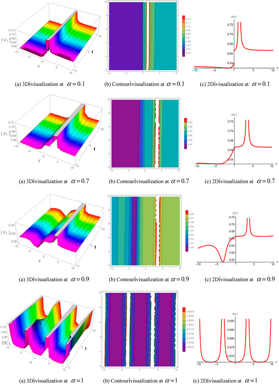
FIGURE 2. Influence of fractional order by 2D, 3D, and corresponding contours of Eq. 36 for $k=2,h=0.6,{\lambda }_0=0.4,{\lambda }_1=-0.2,\beta =0.5,c=0.05,t=1$. $\mathrm{I}\mathrm{f}{\lambda }_0{\lambda }_1>0,$ then

FIGURE 3

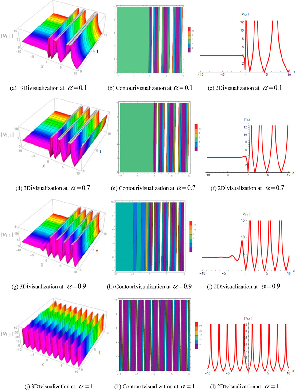
FIGURE 3. Influence of fractional order by 2D, 3D, and corresponding contours of Eq. 42 for $k=2,h=0.6,\lambda =0.5,\beta =0.5,\mu =0.8,\zeta =1,c=0.05,t=1.$

FIGURE 4

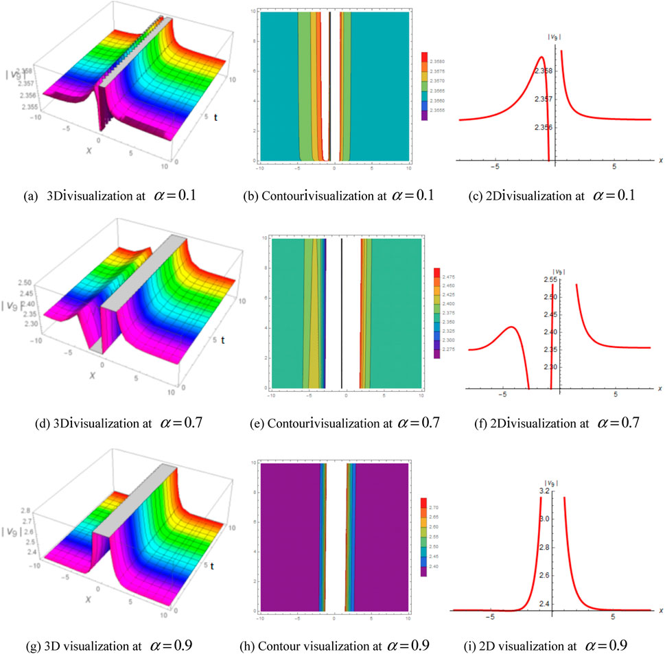
FIGURE 4. Influence of fractional order by 2D, 3D, and corresponding contours of Eq. 57 for $k=2,h=0.6,\lambda =0.5,\beta =0.5,\mu =0.8,\zeta =1,c=0.05,t=1$. For Family 12: When $\zeta =\lambda =K$ and $\mu =0,$

6 Conclusion

In this work, we applied the $\left(G^{\prime }/G,1/G\right)$-expansion, modified the $\left(G^{\prime }/G^2\right)$-expansion, and provided new auxiliary equations methods in a satisfactory way to determine the novel soliton solutions of the space-time fractional LGHE by considering the truncated M-fractional derivative. These methods restored the periodic, singular-kink type, singular-bell shaped, and bright singular wave solutions dark, bright-singular, exponential, trigonometric, and rational solitons. Mathematica was utilized to perform the algebraic computations and generate graphical representations of the obtained solutions at different parameter values. Compared with other works [10, 23], our solutions have not been reported in the previous literature. These techniques are highly effective and robust for discovering soliton solutions for nonlinear fractional differential equations. Furthermore, the solutions obtained can provide deeper insights into the nonlinear dynamics of optical soliton propagation.

Data availability statement

The original contributions presented in the study are included in the article/Supplementary Material. Further inquiries can be directed to the corresponding author.

Author contributions

RZ, W-XM, SA, and IS contributed to the study conception and design. IS and AH organized the database. AH and SA performed the statistical analysis. RZ and KM wrote the first draft of the manuscript. W-XM, IS, and AH wrote sections of the manuscript. SA and AH writing-review and editing. SA is the project administrative. All authors contributed to the article and approved the submitted version.

Funding

This Project is funded by King Saud University, Riyadh, Saudi Arabia.

Acknowledgments

Research Supporting Project number (RSP2023R167), King Saud University, Riyadh, Saudi Arabia.

Conflict of interest

The authors declare that the research was conducted in the absence of any commercial or financial relationships that could be construed as a potential conflict of interest.

Publisher’s note

All claims expressed in this article are solely those of the authors and do not necessarily represent those of their affiliated organizations, or those of the publisher, the editors, and the reviewers. Any product that may be evaluated in this article, or claim that may be made by its manufacturer, is not guaranteed or endorsed by the publisher.

References

1.Wazwaz. Partial differential equations and solitary wave theory. Berlin, Germany: Springer (2009).

Google Scholar

2. Whitham GB. Linear and nonlinear waves. New York: Wiley (1972).

Google Scholar

3. Wazwaz AM. The extended tanh method for abundant solitary wave solutions of nonlinear wave equations. Appl Math Comput (2007) 187:1131–42. doi:10.1016/j.amc.2006.09.013

CrossRef Full Text | Google Scholar

4. Raza N, Zubair A. Bright, dark and dark-singular soliton solutions of nonlinear Schrödinger's equation with spatio-temporal dispersion. J Mod Opt (2018) 65:1975–82. doi:10.1080/09500340.2018.1480066

CrossRef Full Text | Google Scholar

5. Seadawy AR. Two-dimensional interaction of a shear flow with a free surface in a stratified fluid and its solitary-wave solutions via mathematical methods. Eur Phys J Plus (2017) 132:518. doi:10.1140/epjp/i2017-11755-6

CrossRef Full Text | Google Scholar

6. Hosseini K, Sadri K, Mirzazadeh M, Chu YM, Ahmadian A, Pansera BA, et al. A high-order nonlinear Schrödinger equation with the weak non-local nonlinearity and its optical solitons. Results Phys (2021) 23:104035. doi:10.1016/j.rinp.2021.104035

CrossRef Full Text | Google Scholar

7. Hoan LVC, Owyed S, Inc M, Ouahid L, Abdou MA, Chu YM. New explicit optical solitons of fractional nonlinear evolution equation via three different methods. Phys (2020) 18:103209. doi:10.1016/j.rinp.2020.103209

CrossRef Full Text | Google Scholar

8. Rezazadeh H, Ullah N, Akinyemi L, Shah A, Alizamin SMM, Chu YM, et al. Optical soliton solutions of the generalized non-autonomous nonlinear Schrödinger equations by the new Kudryashov’s method. Phys (2021) 24:104179. doi:10.1016/j.rinp.2021.104179

CrossRef Full Text | Google Scholar

9. Hu WP, Deng ZC, Han SM, Fa W. Multi-symplectic Runge-Kutta methods for Landau-Ginzburg-Higgs equation. Appl Math Mech (2009) 30(8):1027–34. doi:10.1007/s10483-009-0809-x

CrossRef Full Text | Google Scholar

10. Bekir1 A, Unsal O. Exact solutions for a class of nonlinear wave equations by using First Integral Method. Int J Nonlinear Sci (2013) 15(2):99–110.

Google Scholar

11. Cyrot M. Ginzburg-Landau theory for superconductors. Rep Prog Phys (1973) 36(2):103–58. doi:10.1088/0034-4885/36/2/001

CrossRef Full Text | Google Scholar

12. Bekir A, Unsal O. Exact solutions for a class of nonlinear wave equations by using the first integral method. Int J Nonlinear Sci (2013) 15(2):99–110.

Google Scholar

13. Iftikhar A, Ghafoor A, Jubair T, Firdous S, Mohyud-Din ST. The expansion method for travelling wave solutions of (2+1)-dimensional generalized KdV, sine Gordon and Landau-Ginzburg-Higgs equation. Sci Res Essays (2013) 8:1349–859.

Google Scholar

14. Barman HK, Akbar MA, Osman MS, Nisar KS, Zakarya M, Abdel-Aty AH, et al. Solutions to the Konopelchenko-Dubrovsky equation and the Landau-Ginzburg-Higgs equation via the generalized Kudryashov technique. Results Phys (2021) 24:104092. doi:10.1016/j.rinp.2021.104092

CrossRef Full Text | Google Scholar

15. Barman HK, Aktar MS, Uddin MH, Akbar MA, Baleanu D, Osman MS. Physically significant wave solutions to the Riemann wave equations and the Landau-Ginsburg-Higgs equation. Results Phys (2021) 27:104517. doi:10.1016/j.rinp.2021.104517

CrossRef Full Text | Google Scholar

16. Islam ME, Akbar MA. Stable wave solutions to the Landau-Ginzburg-Higgs equation and the modified equal width wave equation using the IBSEF method. Arab J Basic Appl Sci (2020) 27(1):270–8. doi:10.1080/25765299.2020.1791466

CrossRef Full Text | Google Scholar

17. Kilbas AA, Srivastava HM, Trujillo JJ. Theory and applications of fractional differential equations. Amsterdam: Elsevier (2006).

Google Scholar

18. Miller S, Ross B. An introduction to the fractional calculus and fractional differential equations. New York, NY: Wiley (1993).

Google Scholar

19. Caputo M, Fabrizio M. A new definition of Fractional differential without singular kernel. Prog Fract Differ Appl (2015) 1(2):1–13.

Google Scholar

20. Khalil R, Horani MA, Yousef A, Sababheh M. A new definition of fractional derivativefinition of fractional derivative. J Compu Appl Math (2014) 264:65–70. doi:10.1016/j.cam.2014.01.002

CrossRef Full Text | Google Scholar

21. Atangana A, Baleanu D, Alsaedi A. Analysis of time-fractional hunter-saxton equation: A model of neumatic liquid crystal. Open Phys (2016) 14:145–9. doi:10.1515/phys-2016-0010

CrossRef Full Text | Google Scholar

22. Vanterler D, Sousa JC, Capelas deOliveira E. A new truncated M-fractional derivative type unifying some fractional derivative types with classical properties. Int J Anal Appli (2018) 16(1):83–96.

Google Scholar

23. Deng SX, Ge XX. Analytical solution to local fractional Landau-Ginzburg-Higgs equation on fractal media. Therm Sci (2021) 25(6B):4449–55. doi:10.2298/tsci2106449d

CrossRef Full Text | Google Scholar

24. Siddique I, Zafar A, Bukht Mehdi K, Osman M, Jaradat A, Zafar KB, et al. Exact traveling wave solutions for two prolific conformable M-Fractional differential equations via three diverse approaches. Results Phys (2021) 28:104557. doi:10.1016/j.rinp.2021.104557

CrossRef Full Text | Google Scholar

25. Siddique I, Mehdi KB, Jaradat MMM, Zafar A, Elbrolosy ME, Elmandouh AA, et al. Bifurcation of some new traveling wave solutions for the time–space M-fractional MEW equation via three altered methods. Results Phys (2022) 41:105896. doi:10.1016/j.rinp.2022.105896

CrossRef Full Text | Google Scholar

26. Sirendaoreji S. Auxiliary equation method and new solutions of Klein–Gordon equations. Chaos Solitons Fractals (2007) 31(4):943–50. doi:10.1016/j.chaos.2005.10.048

CrossRef Full Text | Google Scholar

27. Rezazadeh H, Adel W, Tebue ET, Yao SW, Inc M. Bright and singular soliton solutions to the Atangana-Baleanu fractional system of equations for the ISALWs. J King Saud Univ – Sci (2021) 33:101420. doi:10.1016/j.jksus.2021.101420

CrossRef Full Text | Google Scholar

28. Zayed EME, Abdelaziz MAM. The two variable G'G, 1G-expansion method for solving the nonlinear KdVmKdV equation. Math Prob Engr., ID (2012) 725061:14.

Google Scholar

29. Zhang Y, Zhang L, pang J. Application of G'G2expansion method for solving Schrodinger’s equation with three-order dispersion. Adv Appl Math (2017) 6(2):212–7.

Google Scholar

30. Demiray S, Unsal O, Bekir A. New exact solutions for boussinesq type equations by using (G'/G, 1/G) and (1/G')-Expansion MethodsG'G, 1Gand 1G'expansion method. Acta Phys Pol A (2014) 125(5):1093–8. doi:10.12693/aphyspola.125.1093

CrossRef Full Text | Google Scholar

31. Hafiz Uddin M. Close form solutions of the fractional generalized reaction duffing model and the density dependent fractional diffusion reaction equation. Fractional Diffusion React Equation (2017) 6(4):177–84. doi:10.11648/j.acm.20170604.13

CrossRef Full Text | Google Scholar

32. Wazwaz AM. Couplings of a fifth order nonlinear integrable equation: Multiple kink solutions. Comput Fluids (2013) 84:97–9. doi:10.1016/j.compfluid.2013.05.020

CrossRef Full Text | Google Scholar

33. Wazwaz AM. Kink solutions for three new fifth-order nonlinear equations. Appl Math Model (2014) 38:110–8. doi:10.1016/j.apm.2013.06.009

CrossRef Full Text | Google Scholar

34. Sirisubtawee S, Koonprasert S, Sungnul S. Some applications of the (G′/G,1/G)-Expansion method for finding exact traveling wave solutions of nonlinear fractional evolution EquationsG'G,1Gexpansion method for finding exact traveling wave solutions of nonlinear fractional evolution equations. Symmetry (2019) 11:952. doi:10.3390/sym11080952

CrossRef Full Text | Google Scholar

35. Mahak N, Akram G. Exact solitary wave solutions of the (1+1)-dimensional Fokas-Lenells equation. Optik (2020) 208:164459. doi:10.1016/j.ijleo.2020.164459

CrossRef Full Text | Google Scholar

36. Noufe Aljahdaly H. Some applications of the modified G'G2expansion method in mathematical physics. Results Phys (2019) 13:102272. doi:10.1016/j.rinp.2019.102272

CrossRef Full Text | Google Scholar

37. Daghan D, Donmez O. Exact solutions of the gardner equation and their applications to the different physical plasmas. Braz J Phys (2016) 46:321–33. doi:10.1007/s13538-016-0420-9

CrossRef Full Text | Google Scholar

38. Ali MN, Husnine SM, Saha A, Bhowmik SK, Dhawan S, Ak T. Exact solutions, conservation laws, bifurcation of nonlinear and super nonlinear traveling waves for Sharma-Tasso-Olver equation. Nonlinear Dyn (2018) 94:1791–801. doi:10.1007/s11071-018-4457-x

CrossRef Full Text | Google Scholar

39. Jhangeer A, Almusawa H, Rahman RU. Fractional derivative-based performance analysis to caudrey–dodd–gibbon–sawada–kotera equation. Results Phys (2022) 36:105356. doi:10.1016/j.rinp.2022.105356

CrossRef Full Text | Google Scholar

40. Raza N, Jhangeer A, Rahman R, Butt AR, Chu YM. Sensitive visualization of the fractional wazwaz-benjamin-bona-mahony equation with fractional derivatives: A comparative analysis. Results Phys (2021) 25:104171. doi:10.1016/j.rinp.2021.104171

CrossRef Full Text | Google Scholar

41. Riaz MB, Wojciechowski A, Oros GI, Rahman R. Soliton solutions and sensitive analysis of ModifiedEqual-width equation using fractional operators. Symmetry (2022) 14:1731. doi:10.3390/sym14081731

CrossRef Full Text | Google Scholar