 Huiqiang Tao
 Naveed Anjum
 Yong-Ju Yang3
95% of researchers rate our articles as excellent or good
Learn more about the work of our research integrity team to safeguard the quality of each article we publish.
Find out more
ORIGINAL RESEARCH article
Front. Phys. , 27 April 2023
Sec. Interdisciplinary Physics
Volume 11 - 2023 | https://doi.org/10.3389/fphy.2023.1168795
This article is part of the Research Topic Analytical Methods for Nonlinear Oscillators and Solitary Waves View all 14 articles
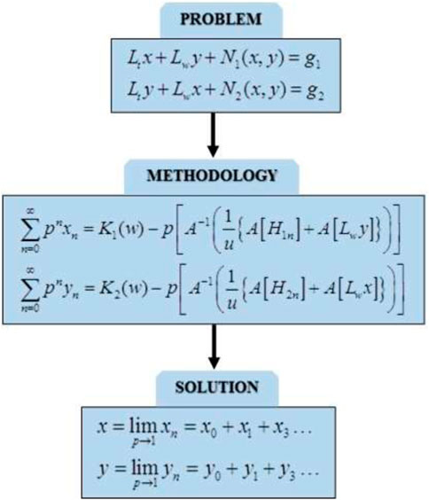
Fractional differential equations can model various complex problems in physics and engineering, but there is no universal method to solve fractional models precisely. This paper offers a new hope for this purpose by coupling the homotopy perturbation method with Aboodh transform. The new hybrid technique leads to a simple approach to finding an approximate solution, which converges fast to the exact one with less computing effort. An example of the fractional casting-mold system is given to elucidate the hope for fractional calculus, and this paper serves as a model for other fractional differential equations.
Fractional calculus has triggered much interest in both physics and mathematics [1, 2]. Traditional differential equations cannot accurately represent many physical problems, and the fractional partner can provide deeper insight into these complex physical phenomena with ease. In general, this newly developed field is for studying real-world applications in the fractal space, so most literature labeled it as the fractal–fractional calculus [3–5] or the local fractional calculus on the Cantor set [6]. A continuum medium, e.g., water or air, becomes a fractal space (porous medium) when we observe it on a molecule’s scale. Any phenomena arising in molecules’ perturbation have to be modeled by the fractal–fractional model [7]. As an example, we consider a nanoparticle’s motion in the air, which is stochastic and difficult to be modeled by the traditional differential equation; however, if the air is considered as a fractal space on a molecule’s scale, its motion is determinate and can be modeled by the fractal–fractional model. So, we need two scales for a porous medium; one is large enough so that the continuum assumption works, and the other is small enough so that the porosity can be measured, as pointed out by Ji-Huan He that “seeing with a single scale is always unbelieving” [8]. Another example is the motion of the Moon, which is naturally periodic; however, if we measure its motion at an extremely far distance, its motion becomes stochastic, and the Heisenberg-like uncertainty principle works for the Moon [9]. He and Qian showed that the fractal diffusion process in water depends on the fractal dimensions [10], and other scientists also discussed the fractional advection–reaction–diffusion process [11] and the fractal diffusion–reaction process [12]. A cocoon’s air/moisture permeability and its thermal property can best be revealed by the fractal–fractional model [13, 14], and the fractal micro-electromechanical systems show even more amazing properties [15–18].
Fractional calculus is a good and reliable tool for scientists and engineers but a mixed blessing for practical applications because an intractable problem arises; that is, fractional models are extremely difficult to be solved. Researchers have been racing to test various analytical methods which were originally proposed to solve traditional differential equations. Though there are many famous analytical methods in the literature, for example, the homotopy perturbation method [19–23] and its various modifications [24–26], the decomposition method [27], the variational iteration method [28–30], the exp-function method [31], and the differential transform method [32], so far, there is not a universal approach to solving exactly fractional differential equations, and this paper offers a new hope for this purpose by coupling the homotopy perturbation method [33, 34] and the Aboodh transform [35].
The homotopy perturbation method (HPM) was first proposed by Chinese mathematician Prof. Ji-Huan He in the later 1990s [33]; it is mathematically simple and physically insightful. The method is equally suitable for linear or non-linear, homogeneous or inhomogeneous, and initial and/or boundary value problems. The solution is expressed in an infinite series and typically converges to the exact solution. The HPM is now considered a matured tool for almost all kinds of problems, and many researchers have used this method for an accurate insight into the solution properties of a complex problem [36–38].
The Aboodh transform (AT) was proposed by Aboodh [35] and derived from the classical Fourier integral. This transform is now considered a simple technique for solving linear differential equations but is unable to solve non-linear ones. By coupling AT with the HPM, one has the capability to solve linear and non-linear problems, and a lot of literature works have been witnessed to utilize this coupling for solving various types of problems. Using AT–HPM, Manimegalai et al. [39] solved strongly non-linear oscillators with great success. Jani and Singh [40] found it had obvious advantages over the decomposition method, Yasmin [41] revealed the dynamic behavior of the fractional convection–reaction–diffusion process, and Jani and Singh [42] extended it to the soliton theory.
Though much work was achieved, in this study, we will show that AT–HPM is a universal tool for fractional calculus. As an example, we consider the time-fractional casting-mold system which is used in manufacturing various medical equipment, ranging from injections to the COVID-19 tool-kit [43]. The significant findings reveal that AT–HPM is an accurate and effective approach that reduces the computational work with fast convergence ratio.
This section is divided into two sections. In the first section, the methodology will be proposed, and the convergence of the suggested technique will be discussed in the second section.
In this section, we give a brief introduction to the Aboodh transform [35] and homotopy perturbation method [33, 34].
If
where
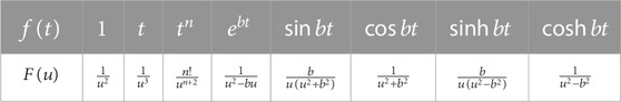
TABLE 1. Aboodh transform of some elementary functions.
The Aboodh transform of the partial derivative of time can be obtained using the following formula:
where
where
where
By employing the differential characteristic of Aboodh transform, we can express Eq. 3 as
and after using the initial conditions, we have
or
where
where
where
By substituting Eqs 7, 8 in Eq. 6, we get
Comparing the coefficients of like powers of
We can obtain the best approximation for the solution as
To show that the series solution of the system in Eq. 14 converges to the solution of Eq. 3, we are to prove the sufficient condition of the convergence, and the following theorem will help us.
Theorem: We assume that X and Y are Banach spaces and
Then, according to Banach’s fixed point theorem, M has a unique fixed point
and considering that
(i)
(ii)
Proof: (i) By the principle of mathematical induction, for
Assuming
By employing the definition of
(ii) As
Hence, the given statement is proved.
In this section, three examples are presented to illustrate the idea explained in Section 2. First, we will study the method for a homogeneous linear system of PDEs. Second, the analytical solution will be obtained for an inhomogeneous linear system of PDEs. Finally, the inhomogeneous non-linear system of PDEs will be examined.
We consider the following linear system:
with initial conditions
By employing the Aboodh transform method, we have
Using the initial conditions given in Eq. 16, we reach
or
The Aboodh transform-based homotopy perturbation method considers a series solution given by
By using the aforestated equation, the system of equations in Eq. 19 gets the form
By comparing like powers of
Hence, the series solution by using Eq. 14 can be expressed as
or in a closed form as
which is the exact solution of Eq. 15.
Suppose the following inhomogeneous linear system of PDEs:
with initial conditions
Applying the Aboodh transform on each side of the equations in Eq. 24 and then putting on the given initial conditions, we obtain
or
By using the Aboodh transform-based homotopy perturbation method, the series solution is expressed by
The system of equations in Eq. 27 gets the following form after employing the aforestated equation:
By comparing the coefficient of like powers of
Therefore, the solution in the form of an infinite series by using Eq. 14 can be expressed as
or in its convergent form as
which is the exact solution of Eq. 24.
Suppose the following inhomogeneous non-linear system of PDEs:
with initial conditions
Employing the Aboodh transform on each side of the equations in Eq. 36 and then applying the given initial conditions give
Taking the inverse Aboodh transform on each side, we obtain
According to the Aboodh transform-based homotopy perturbation method, the solution functions
where the non-linear terms
By comparing the coefficient of like powers of
Therefore, the solution in the form of an infinite series by using Eq. 14 can be expressed as
or in its convergent form as
which is the exact solution of Eq. 36.
Now, we turn back to a time-fractional casting-mold system which models the temperature distribution in the casting and molding processes. For this, two heat conduction equations are used with initial and Dirichlet boundary conditions [45]. The mathematical model is depicted as follows:
where
It is necessary to point out that Eq. 48 was originally studied in [45], where the series solution was presented and no closed-form solution was formulated. Our aim here is to overcome the main shortcomings in [45] and to offer a totally new hope for numerical approximation. To this end, applying the Aboodh transform in the aforementioned system, we have
Now, by inverse Aboodh transformation, we obtain
which can further be written as
According to the standard HPM [33, 34], the solution
By substituting Eq. 52 in Eq. 51, the solution can be written as
Equating coefficients of powers of
The approximate solution can be obtained as
We consider the system expressed in Eq. 48 for the case
By employing Eq. 57, the solution can be written as
The expressions are similar to those obtained by the fractional complex transform [46–49]. In the closed form, we obtain
where
This section is devoted to test the applicability and validity of the suggested technique for the time-fractional casting-mold system over the series-based solution of the same model.
Figures 1, 2 present the errors of the series solutions obtained by the HPM [45] for the fractal dimension β = 1. It is observed that for all the parameters and for both casting and molding processes, the errors grow exponentially for the case of a series solution [45] and can be reduced by adding more terms in the solution. On the other hand, the suggested solution has the exact solution, and there is no chance of error even for a larger range of t. Therefore, based on these findings, we can say that the proposed technique is more effective than the previous method [45].
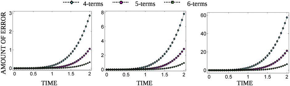
FIGURE 1. Error estimations for the casting process at β = 1 and x = 0.5, 1, 2.
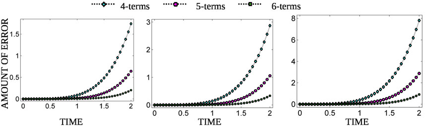
FIGURE 2. Error estimations for the molding process at β = 1 and x = 0.5, 1, 2.
The Aboodh transform-based homotopy perturbation method is successfully employed to solve traditional differential equations and fractional differential equations successfully. This approach has been shown to have the potential to solve both linear and non-linear problems. For a linear system, the exact solution is predicted, while for a non-linear system, with the help of He’s polynomials, a series solution is obtained, which converges fast to the exact one. So, the method pushes the progress of non-linear science and will make a “big change” to increase the number of practical applications, and this paper serves as a model for other applications.
The original contributions presented in the study are included in the article/Supplementary Materials; further inquiries can be directed to the corresponding author.
Conceptualization: HT and NA; methodology: NA and YY; validation: NA and YY; writing—original draft preparation: HT and YY; writing—review and editing: HT, NA, and YY; supervision: HT and YY; and funding acquisition: YY. All authors read and agreed to the published version of the manuscript.
The study was supported by the Natural Science Foundation of Henan Province (No. 222300420507); National Natural Science Foundation of China (No. 12171193), Key Scientific Research Project of High Education Institutions of Henan Province (No. 23A110019), Science and Technology Research Projects of Henan Province (No. 182102110292), Basic and Frontier Technology Research Project of Henan Province (Nos. 12300410398 and 132300410084), and Zhumadian Key Laboratory of Statistical Computing and Data Modeling [No. (2022)12].
The authors declare that the research was conducted in the absence of any commercial or financial relationships that could be construed as a potential conflict of interest.
All claims expressed in this article are solely those of the authors and do not necessarily represent those of their affiliated organizations, or those of the publisher, the editors, and the reviewers. Any product that may be evaluated in this article, or claim that may be made by its manufacturer, is not guaranteed or endorsed by the publisher.
1. Hong BJ. Exact solutions for the conformable fractional coupled nonlinear Schrodinger equations with variable coefficients. J Low Frequency Noise, Vibration Active Control (2023) 146134842211354. doi:10.1177/14613484221135478
2. He JH, He CH, Saeed T. A fractal modification of Chen-Lee-Liu equation and its fractal variational principle. Int J Mode Phys B (2021) 35(21):2150214. doi:10.1142/s0217979221502143
3. Wang KL, Wei CF. Fractal soliton solutions for the fractal-fractional shallow water wave equation arising in ocean engineering. Alexandria Eng J (2023) 65(2023):859–65. doi:10.1016/j.aej.2022.10.024
4. Feng GQ, Niu JY. An analytical solution of the fractal toda oscillator. Results Phys (2023) 44:106208. doi:10.1016/j.rinp.2023.106208
5. He JH, Qie N, He CH. Solitary waves travelling along an unsmooth boundary. Results Phys (2021) 24:104104. doi:10.1016/j.rinp.2021.104104
6. Yang XJ, Srivastava HM, He JH, Baleanu D. Cantor-type cylindrical-coordinate method for differential equations with local fractional derivatives. Phys Lett A (2013) 377(28-30):1696–700. doi:10.1016/j.physleta.2013.04.012
7. He JH. Fractal calculus and its geometrical explanation. Results Phys (2018) 10:272–6. doi:10.1016/j.rinp.2018.06.011
8. He JH. Seeing with a single scale is always unbelieving: From magic to two-scale fractal. Therm Sci (2021) 25(2):1217–9. doi:10.2298/tsci2102217h
9. He JH. Frontier of modern textile engineering and short remarks on some topics in physics. Int J Nonlinear Sci Numer Simulation (2010) 11(7):555–63. doi:10.1515/ijnsns.2010.11.7.555
10. He JH, Qian MY. A fractal approach to the diffusion process of red ink in a saline water. Therm Sci (2022) 26(3B):2447–51. doi:10.2298/tsci2203447h
11. Dai DD, Ban TT, Wang YL, Zhang W. The piecewise reproducing kernel method for the time variable fractional order advection-reaction-diffusion equations. Therm Sci (2021) 25(2B):1261–8. doi:10.2298/tsci200302021d
12. Lin L, Qiao Y. Fractal diffusion-reaction model for a porous electrode. Therm Sci (2021) 25(2):1305–11. doi:10.2298/tsci191212026l
13. Liu FJ, Zhang T, He CH, Tian D. Thermal oscillation arising in a heat shock of a porous hierarchy and its application. Facta Universitatis Ser Mech Eng (2022) 20(3):633–45. doi:10.22190/fume210317054l
14. Xue RJ, Liu FJ. A Fractional model and its application to heat prevention coating with cocoon-like hierarchy. Therm Sci (2022) 26(3):2493–8. doi:10.2298/tsci2203493x
15. Tian D, Ain QT, Anjum N, He CH, Cheng B. Fractal N/MEMS: From pull-in instability to pull-in stability. Fractals (2021) 29:2150030. doi:10.1142/s0218348x21500304
16. Tian D, He CH. A fractal micro-electromechanical system and its pull-in stability. J Low Frequency Noise Vibration Active Control (2021) 40(3):1380–6. doi:10.1177/1461348420984041
17. He JH, Yang Q, He CH, Li HB, Buhe E. Pull-in stability of a fractal MEMS system and its pull-in plateau. Fractals (2023) 30. doi:10.1142/S0218348X22501857
18. He CH. A variational principle for a fractal nano/microelectromechanical (N/MEMS) system. Int J Numer Methods Heat Fluid Flow (2023) 33(1):351–9. doi:10.1108/hff-03-2022-0191
19. Anjum N, He JH. Higher-order homotopy perturbation method for conservative nonlinear oscillators generally and microelectromechanical systems’ oscillators particularly. Int J Mod Phys B (2020) 34:2050313. doi:10.1142/S0217979220503130
20. He CH, El-Dib YO. A heuristic review on the homotopy perturbation method for non-conservative oscillators. J Low Frequency Noise, Vibration Active Control (2022) 41(2):572–603. doi:10.1177/14613484211059264
21. Anjum N, He JH. Homotopy perturbation method for N/MEMS oscillators. Math Methods Appl Sci (2020). doi:10.1002/mma.6583
22. He JH, Jiao ML, He CH. Homotopy perturbation method for fractal Duffing oscillator with arbitrary conditions. Fractals (2023) 30. doi:10.1142/S0218348X22501651
23. He JH, Moatimid GM, Zekry MH. Forced nonlinear oscillator in a fractal space. Facta Universitatis Ser Mech Eng (2022) 20(1):001–20. doi:10.22190/fume220118004h
24. Li XX, He CH (2019). Homotopy perturbation method coupled with the enhanced perturbation method, J Low Frequency Noise Vibration Active Control 38, 1399–403. doi:10.1177/1461348418800554
25. Anjum N, He JH, Ain QT, Tian D. Li-He’s modified homotopy perturbation method for doubly-clamped electrically actuated microbeams-based microelectromechanical system. Facta Universitatis Ser Mech Eng (2021) 19(4):601–12. doi:10.22190/fume210112025a
26. He JH, El-Dib YO. The enhanced homotopy perturbation method for axial vibration of strings. Facta Universitatis Ser Mech Eng (2021) 19(4):735–50. doi:10.22190/fume210125033h
27. Wazwaz AM. The decomposition method applied to systems of partial differential equations and to the reaction–diffusion Brusselator model. Appl Math Comput (2000) 110:251–64. doi:10.1016/s0096-3003(99)00131-9
28. Wang SQ, He JH. Variational iteration method for solving integro-differential equations. Phys Lett A (2007) 367(3):188–91. doi:10.1016/j.physleta.2007.02.049
29. Wang SQ. A variational approach to nonlinear two-point boundary value problems. Comput Math Appl (2009) 58(11):2452–5. doi:10.1016/j.camwa.2009.03.050
30. Shen YY, Huang XX, Kwak K, Yang B, Wang S. Subcarrier-pairing-based resource optimization for OFDM wireless powered relay transmissions with time switching scheme. IEEE Trans Signal Process (2016) 65(5):1130–45. doi:10.1109/tsp.2016.2628351
31. Chen QL, Sun ZQ. The exact solution of the non-linear Schrodinger equation by the exp-function method. Therm Sci (2021) 25(3B):2057–62. doi:10.2298/tsci200301088c
32. Güzel N, Kurulay M. Solution of shiff systems by using differential transform method. Journal of Science and Technology of Dumlupinar University (2008) 16:49–60.
33. He JH. Homotopy perturbation technique. Comp Methods Appl Mech Eng (1999) 178:257–62. doi:10.1016/s0045-7825(99)00018-3
34. He JH, He CH, Alsolami AA. A good initial guess for approximating nonlinear oscillators by the homotopy perturbation method. Facta Universitatis, Ser Mech Eng (2023). doi:10.22190/FUME230108006H
35. Aboodh KS. Application of new transform “Aboodh transform” to partial differential equations. Glob J Pure Appl Math (2014) 10(2):249–54.
36. Peker HA, Cuha FA. Application of Kashuri Fundo transform and homotopy perturbation methods to fractional heat transfer and porous media equations. Therm Sci (2022) 26(4):2877–84. doi:10.2298/tsci2204877p
37. Anjum N, He JH. Two modifications of the homotopy perturbation method for nonlinear oscillators. J Appl Comput Mech (2020) 2020:2482. doi:10.22055/JACM.2020.34850.2482
38. Nadeem M, Li FQ. He-Laplace method for nonlinear vibration systems and nonlinear wave equations. J Low Frequency Noise, Vibration Active Control (2019) 38(3-4):1060–74. doi:10.1177/1461348418818973
39. Manimegalai K, Zephania C F S, Bera PK, Bera P, Das SK, Sil T. Study of strongly nonlinear oscillators using the Aboodh transform and the homotopy perturbation method. Eur Phys J Plus (2019) 134:462–71. doi:10.1140/epjp/i2019-12824-6
40. Jani HP, Singh TR. Aboodh transform homotopy perturbation method for solving fractional-order Newell-Whitehead-Segel equation. Math Methods Appl Sci (2022). doi:10.1002/mma.8886
41. Yasmin H. Application of Aboodh homotopy perturbation transform method for fractional-order convection–reaction–diffusion equation within caputo and atangana–baleanu operators. Symmetry (2023) 15(2):453. doi:10.3390/sym15020453
42. Jani HP, Singh TR. A robust analytical method for regularized long wave equations. Iranian J Sci Technol Trans A: Sci (2022) 46(6):1667–79. doi:10.1007/s40995-022-01380-9
43. Xu RH, Yang LB, Qin Z. Design, manufacture, and testing of customized sterilizable respirator. J Mech Behav Biomed Mater (2022) 131:105248. doi:10.1016/j.jmbbm.2022.105248
44. Ghorbani A. Beyond adomian polynomials: He polynomials. Chaos Solitons Fractals (2009) 39:1486–92. doi:10.1016/j.chaos.2007.06.034
45. Luo XK, Nadeem M, Asjad MI, Abdo MS. A computational approach for the calculation of temperature distribution in casting-mould heterogeneous system with fractional order. Comput Math Methods Med (2022) 2022:1–10. doi:10.1155/2022/3648277
46. Li ZB, He JH. Fractional complex transform for fractional differential equations. Math Comput Appl (2010) 15(5):970–3. doi:10.3390/mca15050970
47. He JH, Elagan SK, Li ZB. Geometrical explanation of the fractional complex transform and derivative chain rule for fractional calculus. Phys Lett A (2012) 376(4):257–9. doi:10.1016/j.physleta.2011.11.030
48. Ain QT, He JH, Anjum N, Ali M. The fractional complex transform: A novel approach to the time-fractional schrödinger equation. Fractals (2021) 28(7):2050141. doi:10.1142/s0218348x20501418
49. He JH, El-Dib YO. A tutorial introduction to the two-scale fractal calculus and its application to the fractal Zhiber-Shabat Oscillator. Fractals (2021) 29:2150268. doi:10.1142/s0218348x21502686
50. Haubold HJ, Mathai AM, Saxena RK. Mittag-leffler functions and their applications. J Appl Math (2011) 2011:1–51. doi:10.1155/2011/298628
Keywords: homotopy perturbation method, Aboodh transform, He’s polynomials, fractional differential equation, two-scale fractal theory
Citation: Tao H, Anjum N and Yang Y-J (2023) The Aboodh transformation-based homotopy perturbation method: new hope for fractional calculus. Front. Phys. 11:1168795. doi: 10.3389/fphy.2023.1168795
Received: 18 February 2023; Accepted: 03 April 2023;
Published: 27 April 2023.
Edited by:
Hamid M. Sedighi, Shahid Chamran University of Ahvaz, IranReviewed by:
Szabolcs Fischer, Széchenyi István University, HungaryCopyright © 2023 Tao, Anjum and Yang. This is an open-access article distributed under the terms of the Creative Commons Attribution License (CC BY). The use, distribution or reproduction in other forums is permitted, provided the original author(s) and the copyright owner(s) are credited and that the original publication in this journal is cited, in accordance with accepted academic practice. No use, distribution or reproduction is permitted which does not comply with these terms.
*Correspondence: Naveed Anjum, eHNuYXZlZWRAeWFob28uY29t
Disclaimer: All claims expressed in this article are solely those of the authors and do not necessarily represent those of their affiliated organizations, or those of the publisher, the editors and the reviewers. Any product that may be evaluated in this article or claim that may be made by its manufacturer is not guaranteed or endorsed by the publisher.
Research integrity at Frontiers
Learn more about the work of our research integrity team to safeguard the quality of each article we publish.