Distinguishable cash, bosonic bitcoin, and fermionic non-fungible token

Modern technology has brought novel types of wealth. In contrast to hard cash, digital currency does not have a physical form. It exists in electronic forms only. To date, it has not been clear what impacts its ongoing growth will have, if any, on wealth distribution. Here, we propose to identify all forms of contemporary wealth into two classes: ‘distinguishable’ or ‘identical’. Traditional tangible moneys are all distinguishable. Financial assets and cryptocurrencies, such as bank deposits and Bitcoin, are boson-like, while non-fungible tokens are fermion-like. We derived their ownership-based distributions in a unified manner. Each class follows essentially the Poisson or the geometric distribution. We contrast their distinct features such as Gini coefficients. Furthermore, aggregating different kinds of wealth corresponds to a weighted convolution where the number of banks matters and Bitcoin follows Bose–Einstein distribution. Our proposal opens a new avenue to understand the deepened inequality in modern economy, which is based on the statistical physics property of wealth rather than the individual ability of owners. We call for verifications with real data.

Introduction

When two one-dollar banknotes are randomly gifted to two people, there occur total four possible ways of distributions. While counting so, it has been naturally assumed that both notes are distinguishable from each other, since they are for sure distinct physical objects, not to mention the different serial numbers printed on them. In contrast, when two cents are credited to a pair of savings bank accounts, there are three possibilities because the two cents as deposits are indistinguishable. Deposits do not have a physical form. They exist in the form of abstract numbers by ‘claim’ and ‘trust’ between the bank and the account holders. While one’s can add up to a natural number, say $k\in \mathbb{N}$,

$1+1+\cdots +1=k,(1)$

all the one’s are intrinsically identical and indistinguishable from one another. The notion of being indistinguishable, or interchangeably identical, is a fundamental property of elementary particles in physics: bosons can share quantum states but fermions subject to the Pauli’s exclusion principle cannot. Consequently, their statistical distributions differ significantly. While the identical property holds certainly for particles at quantum scale, there appears no clear-cut limit of applicability to larger macroscopic objects. In this paper, we propose to identify all kinds of wealth into two classes: distinguishable or identical. All the traditional tangible moneys, i.e., hard cash including minted coins and banknotes, are of physical existence and belong to the distinguishable class. In contrast, financial assets such as bank deposits, stocks, bonds, and loans belong to the boson-like identical class. Furthermore, all the electronic forms of wealth share the identical property. At deep down level of information technology or atomic physics, they comprise of chain of bits which have finite length. The pieces of information stored are accordingly limited mostly to the amounts and, hence, are abstract like the deposit or the natural number (1). With no restriction on the amount of possession, cryptocurrencies, e.g., Bitcoin [1], are boson-like. Contrarily, having unique digital identifiers, non-fungible tokens (NFTs) may be identified as fermions. Having said so, we shall demonstrate that generic identical wealth can be universally and effectively described by Gentile statistics [2] which postulates a cutoff for the maximal amount of possession. It is an established fact that distinguishable, bosonic, and fermionic particles follow, respectively, the Maxwell–Boltzmann, Bose–Einstein, and Fermi–Dirac statistics, which are all about the number of the particles themselves for a given energy. On the contrary, our primary interest in this work is to derive the ownership-based distributions of wealth, i.e., the number of owners who possess a certain amount of wealth, while the owners are assumed to be always distinguishable. Furthermore, it is our working assumption that wealth is distributed in a ‘random’ manner. This should be the case if ideally the owners were all equal. It goes beyond the scope of the present paper to test the hypothesis against real data.

Basic scheme through elemental examples: We start with an elementary example of distributing M number of minted one-cent coins to N number of people in a random manner. We let n_k be the number of people each of whom owns k number of coins, k = 0, 1, 2, ⋯. As we focus on ‘private ownership’ meaning no allowance of sharing, the opposite notion “k_n” does not make sense (except k_n=1), which in a way breaks the symmetry between people and coins both of which are distinguishable. There are two constraints n_k’s satisfy.

$\begin{array}{c}{\sum }_{k=0}^{\infty }{n}_k=N,{\sum }_{k=0}^{\infty }k{n}_k=M.\hfill \end{array}(2)$

Irrespective of our notation, an effective upper bound in the sums exists such as 0 ≤ k ≤ M. Our primary aim is to compute the total number of all possible or ‘degenerate’ ways of distributions for a given set $\left\{\right.n_k’\mathrm{s}\left.\right\}$. Hereafter, generically for any kinds of wealth, we denote such a total number by Ω and further factorize it into two numbers, Ω = ϒ ×Φ, where ϒ is all about the grouping of the owners into $\left\{\right.n_k’\mathrm{s}\left.\right\}$ and, thus, is independent of the sorts of wealth. The properties of wealth are to be reflected in Φ. Specifically, the total number of possible cases for the N number of people to be grouped into n₀, n₁, n₂, ⋯ is

$\mathrm{\Upsilon }=\frac{N!}{n_0!n_1!n_2!\cdots }=\frac{N!}{{\prod }_{k=0}^{\infty }{n}_k!}.(3)$

So, that for the M coins to be grouped into

$\underset{n_1}{\underbrace{\mathrm{1,1},\dots ,1}},\underset{n_2}{\underbrace{\mathrm{2,2},\dots ,2}},\cdots \cdots \underset{n_k}{\underbrace{k,k,\dots ,k}},\cdots (4)$

is, as the coins are distinguishable,

$\mathrm{\Phi }=\frac{M!}{{\left(1!\right)}^{n_1}{\left(2!\right)}^{n_2}\cdots }=\frac{M!}{{\prod }_{k=1}^{\infty }{\left(k!\right)}^{n_k}}.(5)$

Crucially, for each case in ϒ, any of Φ can equally occur. Thus, the total number of possible distributions for a given set $\left\{\right.n_k’\mathrm{s}\left.\right\}$ is the product ϒΦ = Ω. The degeneracy Φ as counted in (5) is significant since it depends on n_k’s. Insignificant degeneracies that are independent of n_k’s may be taken into account which will multiply Φ by an overall constant. For example, extra distinctions depending on whether the distribution of each coin occurs in the morning or afternoon will give an overall factor 2^M to Φ. Yet, our primary interest is to obtain the most probable distribution of n_k. Following the standard analysis in statistical physics at equilibrium, e.g. [3], we shall assume N to be sufficiently large, apply the variation method induced by δn_k to ln Ω = ln ϒ + ln Φ, and acquire the extremal solution. Accordingly, any insignificant degeneracy is independent of n_k’s becomes irrelevant and ignorable. It merely shifts ln Φ by a constant.

We turn to savings accounts. We consider the M cents to be now credited to distinguishable N savings accounts. Since deposits are boson-like identical, the total number of possible distributions Ω is essentially ϒ (3) itself up to multiplying an insignificant overall constant. This irrelevant degeneracy can arise when the bank accounts keep records of all the details of the crediting of the deposits, e.g. the time of transaction, which would make the credited M cents to appear seemingly distinguishable. However, all the information of each credit are recorded in a chain of bits which has a finite length, say l = l₀ + l₁ that decomposes into l₀ for the very record of the amount k and l₁ reserved for any extra information. While the former is rigidly fixed, the extra pieces of information are rather stochastic and, hence, contribute to ln Φ by a constant shift, l₁ ln 2, which is, hence, ignorable.¹

Last, fermion-like wealth or NFTs set M = 1 and, thus, fix the ownership-based distribution rather trivially: $n_k=(N-1){\delta }_k^0+{\delta }_k^1$. Below, for each kind of wealth, we shall introduce what we call the “Gentile” parameter, $\mathrm{\Lambda }\in \mathbb{N}$, which sets an upper bound on the possession number k as 0 ≤ k ≤ Λ and interpolates boson at Λ = ∞ and fermion at Λ = 1. For distinguishable traditional money in a “free’ country, the parameter may be set to coincide with the total number of each kind, e.g., M in (2), or to be less by law. However, electronic forms of wealth can transform to one another. For example, the total amount of deposits at a bank is not fixed due to the external transfers between accounts at different banks. The total amount of each Bitcoin UTXO (Unspent Transaction Output) is not fixed either, since they can “combine” and “split” to other UTXOs [1]. Thus, the total number of each species of identical wealth is not a constant. For this reason and also a technical reason later to justify the approximation of ln n_k! ≃ n_k ln(n_k/e), we shall keep Λ as an independent key parameter which characterizes, as a matter of principle, boson-like or fermion-like identical wealth.

Master formula

For a unifying general analysis, we consider distinguishable and identical wealth together. We call each unit of wealth an object and postulate that there are $D=d+\bar{d}$ distinct kinds of objects: d of them are distinguishable and $\bar{d}$ of them are identical. We label them by a capital index, I = 1, 2, … , D, which decomposes into small ones, $I=(i,d+\bar{ı})$, where i = 1, 2, … , d for the distinguishable species and $\bar{ı}=\mathrm{1,2},\dots ,\bar{d}$ for the identical species. An Ith kind object has value $w_I\in \mathbb{N}$. For example, the present-day euro coin series set d = 8 with w₁ = 1, w₂ = 2, ⋯, w₈ = 200 in the unit of cent. We then denote a generic ownership over them by a D-dimensional non-negative integer-valued vector, $\vec{k}=(k_1,k_2,\dots ,k_D)$ of which each component k_I denotes the number of owned Ith-kind objects and is bounded by a cutoff Gentile parameter: 0 ≤ k_I ≤ Λ_I. In particular, we set Λ_I = ∞ for bosonic I and Λ_I = 1 for fermionic I. We let $n_{\vec{k}}$ be the number of the owners with such a ownership $\vec{k}$. The total number of owners is then

$N=\sum _{\vec{k}}{n}_{\vec{k}}\equiv \sum _{k_1=0}^{{\mathrm{\Lambda }}_1}\sum _{k_2=0}^{{\mathrm{\Lambda }}_2}\cdots \sum _{k_D=0}^{{\mathrm{\Lambda }}_D}{n}_{\vec{k}},(6)$

and the total number of the Ith-kind objects is

$M_I=\sum _{\vec{k}}{k}_I{n}_{\vec{k}}\equiv N{m}_I.(7)$

Hereafter, ${\sum }_{\vec{k}}$ and ${\prod }_{\vec{k}}$ are our shorthand notations for the sum and the product of all k_I’s from zero to Λ_I’s, as in (6) and (8).

On one hand, as the owners are distinguishable, the number of partitions or groupings of the N owners into the different ownerships of $n_{\vec{k}}$’s (6) is, generalizing (3),

$\mathrm{\Upsilon }=\frac{N!}{{\prod }_{\vec{k}}{n}_{\vec{k}}!}\equiv \frac{N!}{{\prod }_{k_1=0}^{{\mathrm{\Lambda }}_1}{\prod }_{k_2=0}^{{\mathrm{\Lambda }}_2}\cdots {\prod }_{k_D=0}^{{\mathrm{\Lambda }}_D}{n}_{\vec{k}}!}.(8)$

On the other hand for the partitions of the objects, only the distinguishable class of objects contributes, as in (5).

$\mathrm{\Phi }=\prod _{i=1}^d\left[\frac{M_i!}{{\prod }_{\vec{k}}{\left(k_i!\right)}^{n_{\vec{k}}}}\right].(9)$

For each partition of owners in ϒ, any of the partitions of distinguishable objects in Φ can equally occur. Therefore, the final, total number of possible outputs for a given set $\left\{\right.n_{\vec{k}}’\mathrm{s}\left.\right\}$ is the product, Ω = ϒ ×Φ.

We proceed to apply the variation method to ln Ω and aim to acquire the extremal solution of $n_{\vec{k}}$. While doing so, there are constraints to impose:

$\begin{array}{c}\delta N={\sum }_{\vec{k}}\delta n_{\vec{k}}=0,\hfill \\ \delta M_i={\sum }_{\vec{k}}{k}_i\delta n_{\vec{k}}=0,\hfill \\ \delta {\bar{M}}_w={\sum }_{\vec{k}}\left({\sum }_{\bar{ı}=1}^{\bar{d}}{w}_{\bar{ı}}{k}_{\bar{ı}}\right)\delta n_{\vec{k}}=0.\hfill \end{array}(10)$

Namely, the total number of owners and those of distinguishable objects of each kind are all conserved, as we assume them to be indestructible. For the identical class of objects, since they may transform to other species, we impose that only their total value

${\bar{M}}_w=\sum _{\vec{k}}\left({\sum }_{\bar{ı}=1}^{\bar{d}}{w}_{\bar{ı}}{k}_{\bar{ı}}\right)n_{\vec{k}}\equiv N{\bar{m}}_w(11)$

is conserved. To proceed, we employ a well-known approximation for the factorial, $\ln n_{\vec{k}}!\simeq n_{\vec{k}}\ln (n_{\vec{k}}/e)$, which is valid for large $n_{\vec{k}}$ only. Our Gentile cutoff parameter Λ_I then effectively prevents $n_{\vec{k}}$ from getting too small, by setting the upper bound on k_I. It follows then, from $\delta \ln n_{\vec{k}}!=\delta n_{\vec{k}}\ln n_{\vec{k}}$, that the variation of ln Ω reads

$\delta \ln \mathrm{\Omega }=-\sum _{\vec{k}}\delta n_{\vec{k}}\left[\ln n_{\vec{k}}+\sum _{i=1}^d\ln \left(k_i!\right)\right]=0.(12)$

Around the extremal distribution, this variation should vanish, while $\delta n_{\vec{k}}$’s must meet the constraints (10), otherwise they are arbitrary. Therefore, only up to some constants $\alpha ,{\beta }_i,\bar{\beta }$, putting

$\alpha \delta N+\left(\sum _{i=1}^d{\beta }_i\delta M_i\right)+\bar{\beta }\delta {\bar{M}}_w-\delta \ln \mathrm{\Omega }=0,(13)$

we should have for every $\vec{k}$ without sum,

$\ln n_{\vec{k}}+\alpha +\sum _{i=1}^d\left[\ln \left(k_i!\right)+{\beta }_i{k}_i\right]+\bar{\beta }\sum _{\bar{ı}=1}^{\bar{d}}{w}_{\bar{ı}}{k}_{\bar{ı}}=0.(14)$

This gives the desired extremal solution.

$\begin{array}{c}{n}_{\vec{k}}=N{P}_{\vec{k}},P_{\vec{k}}=\left[\prod _{i=1}^d{P}_i\left(k_i\right)\right]\left[\prod _{\bar{ı}=1}^{\bar{d}}{\bar{P}}_{\bar{ı}}\left(k_{\bar{ı}}\right)\right],\hfill \end{array}(15)$

where $P_{\vec{k}}$ is our master probability distribution given by the products of Λ-truncated Poisson and geometric distributions.

$\begin{array}{cc}{P}_i\left(k_i\right)={\mathcal{N}}_i\frac{e^{-{\beta }_i{k}_i}}{k_i!},\hfill & {\mathcal{N}}_i=\frac{1}{{\sum }_{k_i=0}^{{\mathrm{\Lambda }}_i}{e}^{-{\beta }_i{k}_i}/k_i!},\hfill \\ {\bar{P}}_{\bar{ı}}\left(k_{\bar{ı}}\right)={\mathcal{N}}_{\bar{ı}}{e}^{-\bar{\beta }{w}_{\bar{ı}}{k}_{\bar{ı}}},\hfill & {\mathcal{N}}_{\bar{ı}}=\frac{1-e^{-\bar{\beta }{w}_{\bar{ı}}}}{1-e^{-\left({\mathrm{\Lambda }}_{\bar{ı}}+1\right)\bar{\beta }{w}_{\bar{ı}}}}.\hfill \end{array}(16)$

To write this, we have solved α in terms of N and the normalization constants, ${\mathcal{N}}_I$’s, such that ${\sum }_{\vec{k}}{P}_{\vec{k}}=1$ and

$\begin{array}{c}\sum _{\vec{k}}{k}_i{P}_{\vec{k}}=\left(1-{\mathcal{N}}_i\frac{e^{-{\beta }_i{\mathrm{\Lambda }}_i}}{{\mathrm{\Lambda }}_i!}\right)e^{-{\beta }_i}=m_i,\hfill \\ \sum _{\vec{k}}{k}_{\bar{ı}}{P}_{\vec{k}}=\frac{1-\left({\mathrm{\Lambda }}_{\bar{ı}}+1\right)e^{-{\mathrm{\Lambda }}_{\bar{ı}}\bar{\beta }{w}_{\bar{ı}}}+{\mathrm{\Lambda }}_{\bar{ı}}{e}^{-\left({\mathrm{\Lambda }}_{\bar{ı}}+1\right)\bar{\beta }{w}_{\bar{ı}}}}{\left(e^{\bar{\beta }{w}_{\bar{ı}}}-1\right)\left[1-e^{-\left({\mathrm{\Lambda }}_{\bar{ı}}+1\right)\bar{\beta }{w}_{\bar{ı}}}\right]}.\hfill \end{array}(17)$

It remains to determine ${\beta }_i,\bar{\beta }$ from (17) and (11). In particular, when Λ_i = ∞, we get $e^{-{\beta }_i}=m_i$ and a precise Poisson distribution holds with ${\mathcal{N}}_i=e^{-m_i}$. On the other hand, when $\bar{d}=1$ and ${\mathrm{\Lambda }}_{\bar{ı}}=\infty$ or ${\mathrm{\Lambda }}_{\bar{ı}}=1$, we obtain $e^{-\bar{\beta }{w}_{\bar{ı}}}=\frac{m_{\bar{ı}}}{1\pm m_{\bar{ı}}}$ and recover the Bose–Einstein or Fermi–Dirac distributions having an exponential tail,

$m_{\bar{ı}}=\sum _{\vec{k}}{k}_{\bar{ı}}{P}_{\vec{k}}=\frac{1}{e^{\bar{\beta }{w}_{\bar{ı}}}\mp 1},(18)$

which quantify the ‘popularity’ (or inverse ‘rarity’ c.f. [4]) of the digital wealth. As the geometric distribution is essentially the exponential Boltzmann–Gibbs law, we may identify $\bar{\beta }$ as the inverse “temperature,” see also [5].

The distribution of the total value follows

$\mathcal{P}\left(v\right)=\sum _{\vec{k}}{\delta }_{\vec{w}\cdot \vec{k}}^v{P}_{\vec{k}},(19)$

where ${\delta }_{\vec{w}\cdot \vec{k}}^v$ is the Kronecker-delta with $\vec{w}\cdot \vec{k}={\sum }_{I=1}^D{w}_I{k}_I$ amounting to a total value v. Essentially (19) is a weighted convolution whose generating function reads for Λ_i = ∞,

$\begin{array}{cc}Z\left(q\right)\hfill & =\sum _{v=0}^{\infty }\mathcal{P}\left(v\right)q^v=\sum _{\vec{k}}{P}_{\vec{k}}{q}^{\vec{w}\cdot \vec{k}}=\left[\prod _{i=1}^d{e}^{m_i\left(q^{w_i}-1\right)}\right]\hfill \\ \multicolumn{3}{c}{\times \left[\prod _{\bar{ı}=1}^{\bar{d}}\left(\frac{e^{\bar{\beta }{w}_{\bar{ı}}}-1}{e^{\bar{\beta }{w}_{\bar{ı}}}-q^{w_{\bar{ı}}}}\right)\left(\frac{e^{\left({\mathrm{\Lambda }}_{\bar{ı}}+1\right)\bar{\beta }{w}_{\bar{ı}}}-q^{\left({\mathrm{\Lambda }}_{\bar{ı}}+1\right)w_{\bar{ı}}}}{e^{\left({\mathrm{\Lambda }}_{\bar{ı}}+1\right)\bar{\beta }{w}_{\bar{ı}}}-1}\right)\right].}\end{array}(20)$

while the truncated Poisson distribution P_i(k_i) (16) with a finite cutoff Λ_i can be applicable to rare valuable items that are not necessarily hard cash; henceforth, for simplicity, we set Λ_i = ∞ (distinguishable) and ${\mathrm{\Lambda }}_{\bar{ı}}=\infty$ (bosonic) or ${\mathrm{\Lambda }}_{\bar{ı}}=1$ (fermionic).² The Poisson and the bosonic/fermionic geometric distributions

$\begin{array}{c}{P}_{\mathrm{p}}\left(m,k\right)=e^{-m}\frac{m^k}{k!},{\bar{P}}_{\mathrm{b}}\left(m,k\right)=\frac{1}{1+m}{\left(\frac{m}{1+m}\right)}^k,\hfill \\ \multicolumn{2}{c}{{\bar{P}}_{\mathrm{f}}\left(m,k\right)=\left(1-m\right){\delta }_k^0+m{\delta }_k^1=\left(1-m\right){\left(\frac{m}{1-m}\right)}^k,}\end{array}(21)$

are then the elemental ‘atomic’ distributions in (16). Here, m > 0 is the mean value in each distribution. For the fermionic distribution, it should be less than one, such as m = 1/N. Furthermore, the variance is m or m(1 ± m) for the distinguishable or bosonic/fermionic cases. In the vanishing limit m → 0, they all reduce to a Kronecker-delta distribution: $P_{\mathrm{p}}(0,k)={\bar{P}}_{\mathrm{b}/\mathrm{f}}(0,k)={\delta }_k^0$.

Poisson versus Geometric: As relevant to both financial assets and cryptocurrencies, here we make various comparisons between P_p(m, k) and ${\bar{P}}_{\mathrm{b}}(m,k)$ allowing arbitrary m > 0 and unrestricted k = 0, 1, 2, … , ∞.

While ${\bar{P}}_{\mathrm{b}}(m,k)$ is a monotonically decreasing function in k, from Stirling’s formula, $\ln k!\simeq k\ln k-k+\ln \sqrt{2\pi k}$, P_p(m, k) assumes the maximal value.

$\mathrm{M}\mathrm{a}\mathrm{x}\left[P_{\mathrm{p}}\left(m,k\right)\right]\simeq 1/\sqrt{2\pi m}\text{at}k\simeq m.(22)$

That is to say, the Poisson distribution is on-peak for the owners of the averaged wealth m = M/N, namely, the ‘middle class’. Furthermore, the ratio of the two distributions

${\bar{P}}_{\mathrm{b}}\left(m,k\right)/P_{\mathrm{p}}\left(m,k\right)=e^{m}k!/{\left(m+1\right)}^{k+1}(23)$

shows that the geometric distribution has a thicker tail than Poisson one for k ≫ m. Yet, complementary to this, an inequality holds:

$\sum _{k>m}{\bar{P}}_{\mathrm{b}}\left(m,k\right)<\sum _{k>m}{P}_{\mathrm{p}}\left(m,k\right),(24)$

which implies that the probability for k > m is larger in the Poisson distribution compared to the geometric one, see Figure 1. In fact, in the large m limit, we have [7]

$\begin{array}{c}\underset{m\to \infty }{\lim }\sum _{k=m+1}^{\infty }{P}_{\mathrm{p}}\left(m,k\right)=\frac{1}{2},\underset{m\to \infty }{\lim }\sum _{k=m+1}^{\infty }{\bar{P}}_{\mathrm{b}}\left(m,k\right)=e^{-1}.\hfill \end{array}(25)$

FIGURE 1

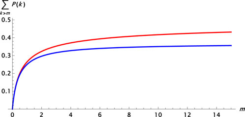
FIGURE 1. The probability to own more than mean value m: ∑_k>mP_p(m, k) (Poisson for distinguishable wealth, red) vs. ${\sum }_{k>m}{\bar{P}}_{\mathrm{b}}(m,k)$ (geometric for identical wealth, blue), with varying mean value m (horizontal axis). The former is always larger than the latter. They converge to 1/2 and e⁻¹ ≃ 0.367879 in the large m limit (25).

Thus, 50% or about 37% of the holders have more than the mean value in the Poisson or geometric distribution.

We compare Shannon entropy, S = ∑_k − P(k) ln P(k). Since, both P(k) and −ln P(k) are non-negative, the entropy is bounded S ≥ 0. The saturation occurs when everyone has the equal amount of wealth i.e. the average value m implying $P(k)={\delta }_k^m$, i.e., either P(k) = 0 or ln P(k) = 0. For the Poisson and geometric distributions, this happens only in the vanishing limit m → 0. For a given arbitrary value of m, it is famously the geometric distribution ${\bar{P}}_{\mathrm{b}}(m,k)$ that sets the entropy maximal,

${\bar{S}}_{\mathrm{b}}\left(m\right)=\left(m+1\right)\ln \left(m+1\right)-m\ln m.(26)$

The entropy of the Poisson distribution P_p(m, k) [8],

$S_{\mathrm{p}}\left(m\right)=\frac{1}{2}\ln \left(2\pi em\right)-\frac{1}{12m}+O\left(m^{-2}\right),(27)$

is then roughly half of the maximum (26) for large m.

We draw the Lorenz curves of P_p(m, k) and ${\bar{P}}_{\mathrm{b}}(m,k)$ as Figures 2, 3, by setting $x={\sum }_{j=0}^{k}P(j)$ and $y=\frac{1}{m}{\sum }_{j=0}^{k}jP(j)$. Since P(0) ≠ 0 in both cases, the curves should include an interval 0 ≤ x ≤ P(0) for trivial y = 0. While, we depict the Lorenz curve of P_p(m, k) numerically, for the geometric distribution ${\bar{P}}_{\mathrm{b}}(m,k)$, we solve for k in terms of x,

$k+1=-\frac{\ln \left(1-x\right)}{\ln \left(1+1/m\right)},(28)$

and obtain an analytic expression of the Lorenz curve:

$y\left(x\right)=\left\{\begin{array}{c}\hfill x+\frac{\left(1-x\right)\ln \left(1-x\right)}{m\ln \left(1+1/m\right)}\text{for}\frac{1}{m+1}\le x<1\hfill \\ 0\text{for}0\le x\le \frac{1}{m+1}\hfill \end{array}\right.,(29)$

of which the large m limit is known [9].

FIGURE 2

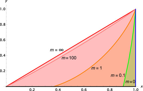
FIGURE 2. Lorenz curves of the Poisson distribution P_p(m, k) for distinguishable wealth. i) m = ∞, ${\mathsf{G}}_{\mathrm{p}}=0$ (45-degree line of perfect equality), ii) m = 100, ${\mathsf{G}}_{\mathrm{p}}\simeq 0.056$, iii) m = 1, ${\mathsf{G}}_{\mathrm{p}}\simeq 0.52$, iv) m = 0.1, ${\mathsf{G}}_{\mathrm{p}}\simeq 0.91$, and v) m = 0, ${\mathsf{G}}_{\mathrm{p}}=1$ as $y={\delta }_x^0$. Each curve includes y = 0 for an interval 0 ≤ x ≤ e^−m. Only when m ≈ 0.35, “80/20 rule” holds.

FIGURE 3

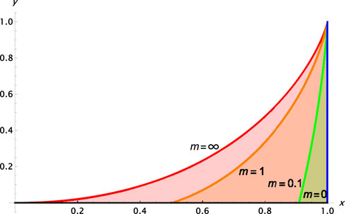
FIGURE 3. Lorenz curves of the geometric distribution ${\bar{P}}_{\mathrm{b}}(m,k)$ for identical wealth. i) m = ∞, ${\mathsf{G}}_{\mathrm{b}}=\frac{1}{2}$ as saturated by y = x + (1 − x) ln(1 − x) [9], ii) m = 1, ${\mathsf{G}}_{\mathrm{b}}\simeq 0.68$, iii) m = 0.1, ${\mathsf{G}}_{\mathrm{b}}\simeq 0.93$, and iv) m = 0, ${\mathsf{G}}_{\mathrm{b}}=1$ as $y={\delta }_x^0$. Each curve includes y = 0 for an interval $0\le x\le \frac{1}{m+1}$. From (29), only when m ≈ 0.47, “80/20 rule (aka Pareto principle)” holds.

At last, we compute the Gini coefficient defined by

$\begin{array}{c}\mathsf{G}[m]≔{\sum }_{k=0}^{\mathrm{\Lambda }}{\sum }_{k^{\prime }=0}^{\mathrm{\Lambda }}\frac{\left|k-k^{\prime }\right|}{2m}P\left(k\right)P\left(k^{\prime }\right)\hfill \\ \hfill & \hfill =1+\frac{1}{m}{\sum }_{k=0}^{\mathrm{\Lambda }}P\left(k\right)\left[kP\left(k\right)-2{\sum }_{k^{\prime }=0}^k{k}^{\prime }P\left(k^{\prime }\right)\right].\end{array}(30)$

For P_p(m, k), from $\frac{1}{{(k!)}^2}=\frac{1}{\pi (2k)!}{\int }_0^{\pi }d\theta {(2\cos \theta )}^{2k}$, we get [10]

${\mathsf{G}}_{\mathrm{p}}\left[m\right]=\frac{1}{\pi }{\int }_0^{\pi }d\theta e^{-2m\left(1-\cos \theta \right)}\left(1+\cos \theta \right).(31)$

For ${\bar{P}}_{\mathrm{b}}(m,k)$ and additionally ${\bar{P}}_{\mathrm{f}}(m,k)$, we have³

$\begin{array}{c}{\mathsf{G}}_{\mathrm{b}}\left[m\right]=\frac{1+m}{1+2m},{\mathsf{G}}_{\mathrm{f}}\left[m\right]=1-m.\hfill \end{array}(32)$

We note then

$\begin{array}{c}\hfill {\mathsf{G}}_{\mathrm{p}}\left[m\right]<{\mathsf{G}}_{\mathrm{b}}\left[m\right]\text{for}\text{\hspace{0.17em}arbitrary\hspace{0.17em}}m>0\text{and}\\ \hfill {\mathsf{G}}_{\mathrm{f}}\left[m\right]<{\mathsf{G}}_{\mathrm{p}}\left[m\right]<{\mathsf{G}}_{\mathrm{b}}\left[m\right]\text{for}0<m<1.\end{array}.(33)$

Especially in the large m limit, we get ${\mathsf{G}}_{\mathrm{p}}[\infty ]=0$ (the perfect equality) and ${\mathsf{G}}_{\mathrm{b}}[\infty ]=\frac{1}{2}$. In the opposite vanishing limit, the Gini coefficients are all unity, ${\mathsf{G}}_{\mathrm{p},\mathrm{b},\mathrm{f}}[0]=1$, hence economically most unequal. Though the fermionic Gini coefficient ${\mathsf{G}}_{\mathrm{f}}[m]=1-m$ can be close to unity as m = 1/N ≪ 1, due to the severe restriction of the possession, i.e. k = 0, 1, it is the smallest among the three.

More than one bank: we now consider the deposits of savings accounts at more than one bank which allow external transfers and adopt the same minimal unit of currency. That corresponds to the equal-weighted convolution (19) of the geometric distributions: with $w_{\bar{ı}}\equiv 1$,

$\begin{array}{c}{\bar{P}}_{\bar{d}}\left(m,k\right)=\frac{\left(\bar{d}+k-1\right)!}{\left(\bar{d}-1\right)!k!}{\left(\frac{\bar{d}}{m+\bar{d}}\right)}^{\bar{d}}{\left(\frac{m}{m+\bar{d}}\right)}^k,\hfill \\ {\bar{Z}}_{\bar{d}}\left(m,q\right)=\sum _{k=0}^{\infty }{\bar{P}}_{\bar{d}}\left(m,k\right)q^k={\left[\frac{\bar{d}}{\bar{d}-m\left(q-1\right)}\right]}^{\bar{d}},\hfill \end{array}(34)$

where $\bar{d}$ is the number of the banks. Remarkably,⁴ for $\bar{d}\ge 2$, ${\bar{P}}_{\bar{d}}(m,k)$ is no longer a monotonically decreasing function in k. It assumes the maximal value,

$\mathrm{M}\mathrm{a}\mathrm{x}\left[P_{\bar{d}}\left(m,k\right)\right]\simeq \frac{1}{\sqrt{2\pi m\left(1-\frac{1}{\bar{d}}\right)\left(1+\frac{m}{\bar{d}}\right)}}\text{at}{k}^{\star }\simeq \left(1-\frac{1}{\bar{d}}\right)m.(35)$

The fact k^⋆ < m implies that ${\bar{P}}_{\bar{d}}(m,k)$ is a more unequal distribution compared to the Poisson one P_p(m, k) (22). Nonetheless, in the large $\bar{d}$ limit, ${\bar{P}}_{\bar{d}}(m,k)$, ${\bar{Z}}_{\bar{d}}(m,q)$, and the maximum (35) all reduce to those of the Poisson distribution or (22),

$\begin{array}{c}\underset{\bar{d}\to \infty }{\lim }{\bar{P}}_{\bar{d}}\left(m,k\right)=e^{-m}\frac{m^k}{k!},\underset{\bar{d}\to \infty }{\lim }{\bar{Z}}_{\bar{d}}\left(m,q\right)=e^{m\left(q-1\right)}.\hfill \end{array}(36)$

An intuitive explanation is as follows. When the number of the banks is infinite, each bank has most likely zero or only one unit of the deposits. The identical wealth then effectively becomes distinguishable by the distinct banks. In this way, ${\bar{P}}_{\bar{d}}(m,k)$ interpolates the geometric and the Poisson distributions, or Figures 2, 3. The more the banks are, the smaller the Gini coefficient is.

Boson-like Bitcoin: As a cryptocurrency, Bitcoin [1] belongs to the identical class of wealth. Although, each UTXO has its unique cryptographic hash, it generates insignificant ignorable pieces of information. UTXOs of a common value are identical, while those of different values are distinguishable, c.f. [11, 12]. The value of every UTXO is discretized in a minimal unit called ‘satoshi’. In this unit, we have $w_{\bar{ı}}\equiv \bar{ı}$ where $\bar{ı}$ runs from one to $\bar{d}=2.1\times 10^{15}$ which is the hard cap encoded in Bitcoin’s source code. For each UTXO worthy of $\bar{ı}$ satoshi, the ownership-based distribution and the expected number are from (16) given by geometric and Bose–Einstein distribution, respectively.

$\begin{array}{c}{\bar{P}}_{\bar{ı}}\left(k_{\bar{ı}}\right)=\left(1-e^{-\bar{ı}\bar{\beta }}\right)e^{-\bar{ı}\bar{\beta }{k}_{\bar{ı}}},\sum _{k_{\bar{ı}}=0}^{\infty }{k}_{\bar{ı}}{\bar{P}}_{\bar{ı}}\left(k_{\bar{ı}}\right)=\frac{1}{e^{\bar{ı}\bar{\beta }}-1}.\hfill \end{array}(37)$

The generating function of the total value (20) is then

$Z\left(q\right)=\prod _{\bar{ı}=1}^{\bar{d}}\frac{1-e^{-\bar{ı}\bar{\beta }}}{1-{\left(e^{-\bar{\beta }}q\right)}^{\bar{ı}}}=\sum _{v=0}^{\infty }\mathcal{P}\left(v\right)q^v,(38)$

and thus, for $v\le \bar{d}$, the total-value-based distribution is

$\begin{array}{c}\mathcal{P}\left(v\right)=\mathcal{P}\left(0\right)\mathfrak{P}\left(v\right)e^{-v\bar{\beta }},\mathcal{P}\left(0\right)=\prod _{\bar{ı}=1}^{\bar{d}}\left(1-e^{-\bar{ı}\bar{\beta }}\right),\hfill \end{array}(39)$

where $\mathfrak{P}(v)$ is the number-theory partition of the non-negative integer v, which appears here since the UTXO values are equally spaced i.e. $w_{\bar{ı}}=\bar{ı}$, as is the case with a simple harmonic quantum oscillator.

We need to determine $\bar{\beta }$ in terms of the mean total value, i.e., ${\bar{m}}_w={\bar{M}}_w/N$ (11).

$\sum _{s=0}^{\infty }s\mathcal{P}\left(s\right)={\left.q{\partial }_{q}Z\left(q\right)\right|}_{q=1}=\sum _{\bar{ı}=1}^{\bar{d}}\frac{\bar{ı}}{e^{\bar{ı}\bar{\beta }}-1}={\bar{m}}_w.(40)$

Practically putting $\bar{d}=\infty$, we approximate the above sum by a semi-infinite integral,

$\sum _{\bar{ı}=1}^{\bar{d}}\frac{\bar{ı}}{e^{\bar{ı}\bar{\beta }}-1}\simeq {\bar{\beta }}^{-2}{\int }_0^{\infty }\text{d}x\frac{x}{e^x-1}=\frac{{\pi }^2}{6{\bar{\beta }}^2},(41)$

and fix $\bar{\beta }$,

$\bar{\beta }\simeq \frac{\pi }{\sqrt{6{\bar{m}}_w}}.(42)$

Furthermore, from the Hardy–Ramanujan formula of the partition, we obtain for large enough v,

$\frac{\mathcal{P}\left(v\right)}{\mathcal{P}\left(0\right)}\simeq \frac{1}{4v\sqrt{3}}{e}^{\pi \sqrt{2v/3}-v\bar{\beta }}(43)$

such that its maximum

$\mathrm{M}\mathrm{a}\mathrm{x}\left[\frac{\mathcal{P}\left(v\right)}{\mathcal{P}\left(0\right)}\right]\simeq \frac{\sqrt{3}{\bar{\beta }}^2}{2{\pi }^2}{e}^{\left({\pi }^2/6\right){\bar{\beta }}^{-1}}(44)$

is positioned at v^⋆ which is smaller than the mean value,

$v^{\star }\simeq \frac{{\pi }^2}{6{\bar{\beta }}^2}{\left(\frac{1+\sqrt{1-24\bar{\beta }/{\pi }^2}}{2}\right)}^2<{\bar{m}}_w=\frac{{\pi }^2}{6{\bar{\beta }}^2}.(45)$

This inequality implies that, despite the large $\bar{d}$ limit which we have tactically assumed, in contrast to the many bank limit (36), the Bitcoin distribution with $w_{\bar{ı}}=\bar{ı}$ is still more unequal than the Poisson one (22): $\mathcal{P}(v)$ (43) has thicker tail than P_p(m, k) ∼ (me/k)^k.

According to [13], as of 2022, the total number of addresses reads N ∼ 10⁹, and the total value of all the UTXOs is roughly ${\bar{M}}_w\sim 10^{15}$ satoshi. We then estimate ${\bar{m}}_w\sim 10^6$ and, from (42), $\bar{\beta }\sim 10^{-3}$, the smallness of which justifies our integral approximation (41).⁵

Discussion: To conclude, traditional tangible moneys are distinguishable; yet financial assets and cryptocurrencies are all identical. The usage of the boson-like wealth results in more unequal geometric-type distribution compared to the Poisson-type distribution of the distinguishable wealth. While so aggregating different kinds of wealth leads to a weighted convolution. In particular, the existence of more than one bank softens the economic inequality of the geometric distribution by a monopolistic bank. Similar to (36) which is for bosonic geometric distributions, the equal-weighted-convolution of fermionic geometric distributions (21) also converges to a Poisson distribution in the large limit of total amount $\bar{M}$ with fixed mean value $m=\bar{M}/N$: the (binomial) convolution

${\bar{P}}_{\bar{M}}\left(m,k\right)=\frac{\bar{M}!}{\left(\bar{M}-k\right)!k!}{\left(1-\frac{1}{N}\right)}^{\bar{M}-k}{\left(\frac{1}{N}\right)}^k(46)$

converges to a Poisson distribution,

$\underset{\bar{M}\to \infty }{\lim }{\bar{P}}_{\bar{M}}\left(m,k\right)=e^{-m}\frac{m^k}{k!}.(47)$

This provides an alternative derivation of the Poisson distribution of distinguishable objects. Even though hard cash is distinguishable, each of them is unique and thus its distribution should coincide with that of NFT, i.e. the fermionic geometric distribution (21). After considering multiple of them of the same value, through the equal-weighted-convolution, the Poisson distribution emerges consistently out of the bosonic as well as fermionic geometric distributions, (36) and (47).

The distribution of Bitcoin is given by the number-theory partition. For completeness, the convolution of a geometric and a Poisson distribution, as for hard cash and savings account, reads

$\begin{array}{c}\widehat{P}\left(m,\bar{m},k\right)≔\sum _{j=0}^{k}P\left(m,j\right)\bar{P}\left(\bar{m},k-j\right)\hfill \\ \hfill & \hfill =\frac{e^{-m}}{\bar{m}+1}{\left(\frac{\bar{m}}{\bar{m}+1}\right)}^k\sum _{j=0}^k\frac{1}{j!}{\left(m+m/\bar{m}\right)}^j,\end{array}(48)$

which carries a power-law tail $\frac{e^{m/\bar{m}}}{\bar{m}+1}{\left(\frac{\bar{m}}{\bar{m}+1}\right)}^k$ for large k.

Putting $w_{\bar{ı}}=1$ and $w_{\bar{ı}}=-1$ separately for a pair of ${\bar{P}}_{\bar{d}}(m,k)$’s (34), we can further aggregate deposit and debt: for net balance $a\in \mathbb{Z}$, we have

${\mathcal{P}}_{\bar{d}}\left(m_1,m_2,a\right)≔\sum _{k_1=0}^{\infty }\sum _{k_2=0}^{\infty }{\delta }_{k_1-k_2}^a{\mathcal{P}}_{\bar{d}}\left(m_1,k_1\right){\mathcal{P}}_{\bar{d}}\left(m_2,k_2\right),(49)$

where m₁ ≥ 0 and m₂ ≥ 0 are the mean values of deposit and debt respectively. In particular, for $\bar{d}=1$, we get

${\mathcal{P}}_{\bar{d}=1}\left(m_1,m_2,a\right)=\left\{\begin{array}{c}\frac{1}{m_1+m_2+1}{\left(\frac{m_1}{m_1+1}\right)}^a\text{\hspace{0.17em}for\hspace{0.17em}}a\ge 0\hfill \\ \frac{1}{m_1+m_2+1}{\left(\frac{m_2}{m_2+1}\right)}^{\left|a\right|}\text{\hspace{0.17em}for\hspace{0.17em}}a<0.\hfill \end{array}\right.(50)$

A priori, the Poisson and geometric distributions (21) depend on the mean ‘number’ m = M/N (dimensionless), rather than any ‘value’ (“dimensionful”). Therefore, any adjustment of the minimal unit, e.g., demolishing cents and keeping euros only, can change the number M and affect the distributions.

It would be of interest to investigate any phase transition for the master distribution (15) through the changes of variables, even if N is finite [14]. As Bitcoin is boson-like, one may wonder about Bose–Einstein condensation especially to the minimal $\bar{ı}=1$ UTXO. For this, we consider its popularity normalized by the mean total value (40), or the ratio $\frac{1}{e^{\bar{\beta }}-1}/\left[{\sum }_{\bar{ı}=1}^{\infty }\frac{\bar{ı}}{e^{\bar{ı}\bar{\beta }}-1}\right]$. This quantity increases monotonically from zero at $\bar{\beta }=0$ and converges to one as $\bar{\beta }$ grows. In particular, when $\bar{\beta }\ge 3$, it becomes greater than 0.9. This “low temperature” might be attainable if Bitcoin gets ever extremely popular: (somewhat unrealistically) large N with ${\bar{M}}_w$ bounded by the hard cap.

We have restricted our work to be theoretical. Yet, the resulting distributions including Figure 2, 3 appear consistent with real data, for example [15–17]. In addition, the (truncated) Poisson-type distribution (16) can be applied not only to tangible moneys, but also to various objects, including citations of research papers [18].

Taking into account the individual differences of owners, or other extra factors, may weaken the assumed ‘randomness’. Even so, we expect that the difference of inequality in distributions persists depending on the class of wealth, distinguishable or identical. We call for thorough verifications with wide applications.

Last, while we have borrowed the notion of indistinguishability from particle and statistical physics for the description of financial wealth, namely, econophysics [19–21], our results such as (36) may help to understand how macroscopic objects formed by many identical particles appear distinguishable, i.e., through the generation of large degeneracy of quantum states.

Data availability statement

The original contributions presented in the study are included in the article; further inquiries can be directed to the corresponding author.

Author contributions

J-HP conceived the idea of identical wealth and derived the distributions. ZYK brought the cryptocurrencies and electronic tokens to the project.

Funding

This study was supported by the Basic Science Research Program through the National Research Foundation of Korea (NRF) Grants NRF-2016R1D1A1B01015196 and NRF-2020R1A6A1A03047877 (Center for Quantum Spacetime).

Acknowledgments

The authors wish to thank Marc Jourdan, Chunghyoung Lee, Sukgeun Lee, Hocheol Lee, and Glassnode Support Team for helpful communications. This work was supported by the Basic Science Research Program through the National Research Foundation of Korea (NRF) Grants NRF-2016R1D1A1B01015196 and NRF-2020R1A6A1A03047877 (Center for Quantum Spacetime).

Conflict of interest

The authors declare that the research was conducted in the absence of any commercial or financial relationships that could be construed as a potential conflict of interest.

Publisher’s note

All claims expressed in this article are solely those of the authors and do not necessarily represent those of their affiliated organizations, or those of the publisher, the editors, and the reviewers. Any product that may be evaluated in this article, or claim that may be made by its manufacturer, is not guaranteed or endorsed by the publisher.

Footnotes

¹In this reason, we prefer to say credits are boson-like rather than (precisely) bosons. Furthermore, we note that the extra pieces of information are generically postdictive: they do not preexist before the transactions take place, or before the ownerships settle down.

²The geometric distribution ${\bar{P}}_{\bar{ı}}(k_{\bar{ı}})$ with other finite values of ${\mathrm{\Lambda }}_{\bar{ı}}$ appears applicable to some Ethereum’s flexible token standard (ERC-1155) [6].

³Alternative to (30), we may compute the Gini coefficient through an integral of the Lorenz curve (29),

${\mathsf{G}}_{\mathrm{b}}^{\prime }\left[m\right]={\left(\frac{m}{m+1}\right)}^2\left(\frac{1}{2m\ln \left(1+1/m\right)}+\frac{1}{m}+\frac{1}{m^2}\right),$

which differs from ${\mathsf{G}}_{\mathrm{b}}[m]$ in (32) by at most 2.4% at m ≃ 0.53.

⁴In contrast, rather natural from the very distinguishability, the equal-weighted convolution of the Poisson distributions is closed:

$\sum _{l=0}^k{P}_{\mathrm{p}}\left(m_1,l\right)P_{\mathrm{p}}\left(m_2,k-l\right)=P_{\mathrm{p}}\left(m_1+m_2,k\right).$

⁵For $\bar{\beta }=10^{-3}$ and $\bar{d}\ge 10^4$, the error of (41) is less than 0.1%.

References

1. Nakamoto S. Bitcoin: A peer-to-peer electronic cash system. Available at: https://bitcoin.org/en/https://bitcoin.org/bitcoin.pdf (Accessed October 31, 2008).

Google Scholar

2. Gentile J. itOsservazioni sopra le statistiche intermedie. Nuovo Cim (1940) 17:493–7. doi:10.1007/BF02960187

CrossRef Full Text | Google Scholar

3. Huang K. Introduction to statistical physics. Chapman and Hall/CRC (2009). doi:10.1201/9781439878132

CrossRef Full Text | Google Scholar

4. Mekacher A, Bracci A, Nadini M, Martino M, Alessandretti L, Aiello LM, et al. Heterogeneous rarity patterns drive price dynamics in NFT collections. Sci Rep (2022) 12:13890. doi:10.1038/s41598-022-17922-5

PubMed Abstract | CrossRef Full Text | Google Scholar

5. Dragulescu A, Yakovenko VM. Statistical mechanics of money. Eur Phys J B-Condensed Matter Complex Syst (2000) 174:723–9. doi:10.1007/s100510070114

CrossRef Full Text | Google Scholar

6.Multi Token Standard ERC-1155. The Ethereum improvement proposal repository. Multi Token Standard ERC-1155 (2018). Available at: https://github.com/ethereum/EIPs/issues/1155.

Google Scholar

7.NIST. NIST digital library of mathematical functions (2022). Available at: https://dlmf.nist.gov/8.11.

Google Scholar

8. Evans RJ, Boersma J. The entropy of a Poisson distribution (C. Robert Appledorn). SIAM Rev (1988) 30(2):314–7. doi:10.1137/1030059

CrossRef Full Text | Google Scholar

9. Dragulescu A, Yakovenko VM. Evidence for the exponential distribution of income in the USA. Eur Phys J B-Condensed Matter Complex Syst (2001) 20:585–9. doi:10.1007/pl00011112

CrossRef Full Text | Google Scholar

10. Ramasubban TA. The mean difference and the mean deviation of some discontinuous distributions. Biometrika (1958) 45(3-4):549–56. doi:10.1093/biomet/45.3-4.549

CrossRef Full Text | Google Scholar

11. Kahn CM. Tokens vs. accounts: Why the distinction still matters, on the economy. Federal Reserve Bank of St. Louis (2020). Available at: https://www.stlouisfed.org/on-the-economy/2020/october/tokens-accounts-why-distinction-matters.

Google Scholar

12. Milne AKL. Argument by false analogy: The mistaken classification of Bitcoin as token money. Available at SSRN: https://ssrn.com/abstract=3290325 (Accessed November 25, 2018).

Google Scholar

13.Studio Glassnode. Studio Glassnode (2022). Available at: https://studio.glassnode.com/metrics?a=BTC.

Google Scholar

14. Park J-H, Kim SW. Thermodynamic instability and first-order phase transition in an ideal Bose gas. Phys Rev A (2010) 81:063636. doi:10.1103/PhysRevA.81.063636

CrossRef Full Text | Google Scholar

15. Lundberg J, Waldenström D. Wealth inequality in Sweden: What can we learn from capitalized income tax data? Rev Income Wealth (2018) 64:517–41. doi:10.1111/roiw.12294

CrossRef Full Text | Google Scholar

16. Juelsrud RE. Deposit concentration at financial intermediaries. Econ Lett (2021) 199(2021):109719. ISSN 0165-1765. doi:10.1016/j.econlet.2020.109719

CrossRef Full Text | Google Scholar

17. Dragulescu A, Yakovenko VM. Exponential and power-law probability distributions of wealth and income in the United Kingdom and the United States. Physica A: Stat Mech its Appl (2001) 2991-2:213–21. doi:10.1016/s0378-4371(01)00298-9

CrossRef Full Text | Google Scholar

18. Berg J. Journal impact factors –Fitting citation distribution curves. Blog-post, Science (2016). Available at https://www.science.org/content/blog-post/journal-impact-factors—fitting-citation-distribution-curves.

Google Scholar

19. Mantegna R, Stanley HE. Introduction to econophysics. Cambridge University Press (1999). Available at: https://EconPapers.repec.org.

Google Scholar

20. Stanley HE, Amaral LAN, Canning D, Gopikrishnan P, Liu Y. Econophysics: Can physicists contribute to the science of economics? Physica A: Stat Mech its Appl (1999) 269(1):156–69. ISSN 0378-4371. doi:10.1016/S0378-4371(99)00185-5

CrossRef Full Text | Google Scholar

21. Buchanan M. What has econophysics ever done for us? Nat Phys (2013) 9:317. doi:10.1038/nphys2648

CrossRef Full Text | Google Scholar