 Lei Fu
 Jingjing Li
 Hongwei Yang
 Xiaofeng Han
94% of researchers rate our articles as excellent or good
Learn more about the work of our research integrity team to safeguard the quality of each article we publish.
Find out more
ORIGINAL RESEARCH article
Front. Phys., 06 February 2023
Sec. Interdisciplinary Physics
Volume 11 - 2023 | https://doi.org/10.3389/fphy.2023.1108505
This article is part of the Research TopicNonlocal Integrable System and Nonlinear WavesView all 8 articles
The nonlinear Schrödinger (NLS) equation is an ideal model for describing optical soliton transmission. This paper first introduces an integer-order generalized coupled NLS equation describing optical solitons in birefringence fibers. Secondly, the semi-inverse and fractional variational method is used to extend the integer-order model to the space–time fractional order. Moreover, various nonlinear forms of fractional NLS equations are discussed, including the Kerr, power, parabolic, dual-power, and log law. The exact soliton solutions, such as bright, dark, and singular solitons, are given. Finally, the behavior of the solution is shown by three-dimensional figures with different fractional orders, which reveals the propagation characteristics of optical solitons in birefringence fibers described by the generalized coupled space–time fractional NLS equation.
With the great progress of the information technology and the increase in market demand, especially with the outbreak of COVID-19 in recent years, modern society relies more and more on communication, forcing optical fiber communication to develop to high-speed and large capacity. Optical fiber communication has become the main transmission mode of communication network due to its high transmission capacity, low loss, and wide frequency band. Optical soliton is the most ideal information carriers in fiber optic communications. From the perspective of physics, optical solitons can keep the waveform and speed of optical fiber transmission unchanged, which is a special product of non-linear effects in optics. It is considered one of the most promising transmission modes in the next generation [1]. From the perspective of mathematics, optical solitons are integrable solutions of some non-linear partial differential equations. Studying the exact solution of these mathematical models has become a great significant frontier in this field [2, 3].
In the field of optical fiber communication, NLS-type equations have attracted great attention from researchers [4–6]. In the 1850s and 1860s, the NLS equation was introduced to study the two-dimensional self-focusing phenomenon of strong beams in weakly interacting non-ideal Bose gases and non-linear media. As a general equation to reveal the propagation of wave packets in weakly non-linear medium, the NLS equation is of great significance to the study of non-linear physics. With further research, the NLS equation has been extended to the equations of the variable coefficient, complex coefficient, multi-dimensional, higher order, non-local, and fractional order, which contain various physical effects [7, 8]. The standard NLS equation contains a second-order dispersion term and a third-order non-linear term [9–11], in the form of
The aforementioned equation describes the picosecond pulse propagation in a single-mode fiber without ignoring the optical loss. Here, u = u(x, t) represents the complex function of the real variables x and t. Both p and q are non-zero real numbers, representing the group velocity dispersion coefficient and self-phase modulation coefficient, respectively. The subscripts represent the corresponding partial derivatives.
Introducing birefringence, a natural phenomenon in fiber optics, into fiber optics will contribute to improve the research and development of high-birefringence fibers. The Kerr, power, parabola, and dual-power non-linearity laws are considered to study solitons in birefringent fibers. These criteria for the existence of solitons are also regarded as constraints [12, 13]. In birefringent fibers, the basic theoretical model of optical pulse transmission is coupled NLS equations [14, 15]. The classical coupled NLS equations have the following form:
where u1 and u2 represent the slow-varying amplitude of two interacting fiber modes; the coupled NLS equations include not only self-similar modulation |u1|2u1 and |u2|2u2 but also cross-phase modulation |u1|2u2 and |u2|2u1.
Fractional calculus plays an important role in physics and engineering. Fractional derivatives have been successfully used to describe fractal problems in engineering, such as the heat transfer in fractal medium [16], fractal hydrodynamic equations [17], fractal electrostatics [18], fractal Fokker–Planck equations [19], fractal description of stress, and strain in elasticity [20] [21–23].
In 2000, Laskin first proposed fractional quantum mechanics [24], which replaced the traditional NLS equation with a fractional NLS equation of the generalized second-order partial differential equation with a fractional order. The fractional NLS equation has attracted extensive attention in the field of physics [25, 26]. It has important implications for theoretical research in the field of fraction and fractional spin particle dynamics [27]. The theory of fractional NLS equations is difficult to advance due to the influence of its inherent non-local operators and the connection between fractional derivatives. Until 2015, Longhi considered the similarity between the Schrodinger equation and the paraxial wave equation. Then, the fractional NLS equation is introduced into optics, and the quantum harmonic oscillator is simulated by optical methods [28]. The field of optics provides a wealth of possibilities for the realization of the fractional NLS equation theory and the study of fractional transmission dynamics of light beams [29–31].
This paper is organized as follows: in Section 2, the generalized coupled spatiotemporal fractional NLS equations are derived using the semi-inverse and Agrawal’s method [32, 33]. Kerr, power, parabolic, dual-power, and log laws of this equations are discussed, and bright, dark, and singular solitons are obtained by changing the amplitude components of the function [34–37]; in Section 3, the behaviors of the obtained solutions are shown by three-dimensional graphics with four different fractional orders; and in Section 4, we elaborate the conclusion of this paper.
In this section, with a fractional derivative theory, we derive the two-dimensional coupled fractional NLS equations in the fractal domain by the Euler–Lagrange equation, and semi-inverse and Agrawal’s variation methods. The generalized coupled NLS equations under the rigid-lid assumption are
where u(x, t) and v(x, t) are complex valued functions that denote the soliton profiles for the two components in birefringent fibers, F is a non-linear function, al(l = 1, 2) denotes the group velocity dispersion coefficients, bl(l = 1, 2) denotes the space–time dispersion terms, and cl and dl(l = 1, 2) denote the self-phase and cross-phase modulation terms, respectively. In the perturbation terms, λl(l = 1, 2) denotes non-linear dispersion and θl(l = 1, 2) represents the third-order dispersion which should be considered when the situation of the group velocity dispersion is small.
The coupled space–time fractional NLS equations can be represented by the following equations. We assume the potential function u(x, t) = f(x, t) + ig(x, t) and v(x, t) = p(x, t) + iq(x, t) accordingly that Eq. 1 has the following form:
where the subscripts represent the partial differential function with parameters.
The function of the potential Eq. 2 can be expressed as
The coefficients ci, di, mi, and ni (i = 1, 2, …, 6) are Lagrange multipliers. The integral shown in Eq. 3 can be calculated by fx|R = fx|T = 0, gx|R = gx|T = 0, px|R = px|T = 0, and qx|R = qx|T = 0, respectively. |u|2 and |v|2 and the function F is treated as a fixed function.
On the basis of the function conversion, we get the following relationship by using variational optimization conditions and δJ(f, g, p, q) = 0 for piecewise integration:
Compared with Eq. 3, in the aforementioned Eq. 4, we get
Similarly, the Lagrangian form of the coupled space–time fractional NLS equations can be converted as
where
Here, Γ(x) is the standard Euler’s gamma function.
The functional form of the coupled fractional NLS equations is
in which
The relationship can be obtained by integration by parts [40].
With δJ(A, B, M, N) = 0, we obtain the Euler–Lagrangian equations of coupled NLS equations in the form
Substituting the Lagrange form of the NLS equations (Eq. 6) into the Euler–Lagrange formula (Eq. 11) and defining u(x, t) = A(x, t) + iB(x, t) and v(x, t) = M(x, t) + iN(x, t) according to the definition of the fractional potential function yields
where α and β are fractal dimensions and u(x, t) and v(x, t) denote the fractal wave functions for space x and time t. Equation 12 is the generalized coupled space–time fractional NLS equations.
We obtain the soliton solution of the equation by using the solitary wave ansatz to perform the integration of the coupled fractional NLS equations (Eq. 12) in this section. It is considered that the four types of non-linear conditions of the equation are the Kerr, power, parabolic, dual-power, and log power non-linearity laws.
Introducing the fractional transforms yields
where m1 and m2 are constants. With the aforementioned conversions, the fractional derivatives are transformed into the classic derivatives [41] as
According to Eqs 12–14, it becomes
The Kerr law non-linearity is also called cubic non-linear. This non-linearity occurs when the light wave in the fiber is subjected to a non-linear response. According to the Kerr law non-linearity F(s) = s, Eq. 15 describes the propagation of dispersive solitons and can be rewritten as
We obtain the exact bright, dark, and singular 1-soliton solutions of the coupling equations by the ansatz method, respectively. To set the starting point, we write the solitons as the phase-amplitude form, similar to [38].
where Pl(X, T)(l = 1, 2) denotes the amplitude components of the soliton solution. The phase component ϕ(X, T) is
where κ represents the frequency, and ω and σ denote the wave number and phase constant, respectively. Substituting Eq. 17 into Eq. 16 and decomposing this equation into real and imaginary parts yield
and
respectively, with l = 1, 2 and
provided
It is important to note a special situation where θl = λl = 0. One study on recovering from a non-dispersive situation was reported in 2014 [22].
The coefficients of the linear components in Eq. 16 can be calculated by comparing the two result values of the soliton velocities as follows:
Eq. 21 becomes
Without considering the non-linearity, Eqs 19, 20 take the following new form as
and
To solve the bright solitons, the starting assumption is [42]
with l = 1, 2 and
where Al and B represent the amplitude and inverse width of the solitons, respectively; v is the soliton velocity, which is considered to be the same along the two components. Substituting Eq. 27 into Eq. 25 yields
On account of the equilibrium principle [38] and applying it to the real part, Eq. 29 can be transformed into
Thus,
with l = 1, 2. Considering the linearly independent functions sechjτ with zero coefficients, when j = 1, 3, the velocity and wave numbers of the resulting bright solitons are
When bB ≠ 0 and bκ ≠ 1, it is noted that the two replacement expressions of the soliton velocity v are equal to l = 1, 2 in Eq. 32; the relationship between Al and A2 is
constrained by
With Eq. 34, comparing Eqs 24–33 yields
With l = 1, 2 and
Therefore, the bright soliton solutions for the Kerr law non-linearity of the generalized coupled fractional NLS equations are
The parameters and corresponding constraints in the formula are consistent with the aforementioned discussion.
Figure 1 shows the 3D plots of bright soliton solutions for the Kerr law non-linearity with the four different fractional values: 0.15, 0.45, 0.75, and 1. Bright solitons depict solitary waves with peak intensities higher than those on the ground. Moreover, it can be clearly found that when changing the values of the fractional orders α and β, the contours and widths of the soliton solutions all change. With the increase of α and β, the widths of the solitons change irregularly and the plots gradually become smooth.
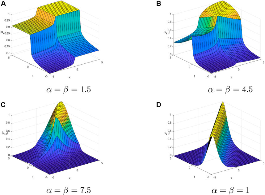
FIGURE 1. 3D plots of bright soliton solutions for the Kerr law non-linearity with the four different fractional values by considering the values A1 = 1, B = −1, v = 1, κ = −1, ω = 3, and δ = 1. (A) α = β = 1.5. (B) α = β = 4.5. (C) α = β = 7.5. (D) α = β = 1.
To solve the dark solitons, from the assumption [36],
where the argument τ is given in Eq. 28. The substitution of Eq. 39 into Eq. 16 leads to
The equilibrium principle reveals the same values of pl with l = 1, 2 as Eq. 31. Analogously, as to bright solitons, considering the coefficients of the linearly independent functions of Eq. 40 yields
It should be noted that in Eq. 41, the specific value between amplitudes shows the same relationship given in Eqs 34, 35 by contrasting the wave velocity v with l = 1, 2.
Considering Eq. 34, two possible expressions of the velocity in Eqs 24, 42 are jointly evaluated for either value of l, and we get
as long as
Therefore, the dark soliton solutions for Kerr law non-linearity are
where Eq. 43 describes the soliton amplitudes, Eqs 41, 42 describe the velocity and the wave numbers, and Eq. 34 describes the frequency accompanied by corresponding constraints.
Figure 2 shows dark soliton solutions for Kerr law non-linearity with the four different fractional values. Dark solitons depict solitary waves whose intensity is lower than that of the background. As can be seen from Figures 2A–D, with the increase of α and β, the amplitudes of solitons increase, while their widths change irregularly. When α = β = 1, the soliton has the largest amplitude.
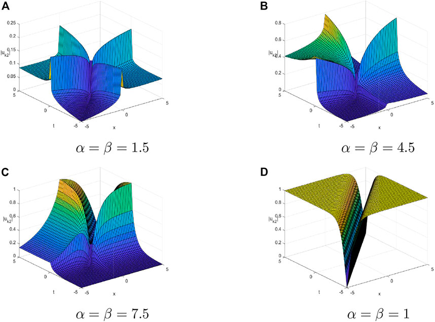
FIGURE 2. 3D plots of dark soliton solutions for the Kerr law non-linearity with the four different fractional values by considering the values A1 = 1, B = −1, v = 1, κ = −1, ω = 3, and δ = 1. (A) α = β = 1.5. (B) α = β = 4.5. (C) α = β = 7.5. (D) α = β = 1.
To solve the singular solitons, the assumption is [36]
where Al denotes the pulse amplitude and pl is a free parameter to be evaluated by the equilibrium non-linearity and will be revealed in the following. Substituting Eq. 46 into Eq. 16 leads to
After the equilibrium program, we get the values of the parameter pl in Eq. 31. It can also be evaluated in coefficients of independent elements
Considering Eq. 34 and equalizing the two possible velocity expressions Eqs. 24, 48, we obtain
with l = 1, 2 and
The singular 1-soliton solutions for Kerr law non-linearity are
If the corresponding constraints, as described previously are satisfied, the singular soliton solution will persist.
In physics research, various materials exhibit power law non-linearities, such as semiconductors. This non-linear law occurs in non-linear plasmas and can solve the small K-condensation problem theory in weak turbulence. The general form of a non-linear function is F(s) = sn, where n denotes a parameter of power law non-linear. We restrict 0 < n < 2 to ensure the wave stability and n ≠ 2 to avoid self-focusing singularities, the initial system Eq. 15 can be rewritten as
Substituting Eq. 17 into Eq. 52 and transforming the real part Eq. 19 into
The imaginary part takes the form as
The real part of Eq. 53 can be simply written as
We use the same starting assumption as the cubic nonlinearity given by Eqs 27, 28 to conduct research on the bright soliton solutions on the system (Eq. 52). Substituting Eq. 27 into Eq. 55 yields
From the equilibrium between nonlinearity and dispersion,
where
with l = 1, 2. Substituting Eq. 58 into Eq. 56 and letting the coefficients set to zero of the linearly independent functions sechjτ with
and
when bB ≠ 0 and bκ ≠ 1; in Eq. 59, by equating the two alternative expressions for the soliton velocity v with 1 = 1, 2, the relation form between the amplitudes can be written as
with l = 1, 2,
whenever the inequality Eq. 37 holds. Hence, the bright soliton solutions for power law nonlinearity of the generalized coupled fractional NLS equations are
The aforementioned conditions determine the perturbation of the bright soliton solutions.
Dark solitons are applied to the same ansatz method in Eq. 39; the real part equation Eq. 55 can be transformed into
The equilibrium principle can calculate the value of pl, as shown in Eq. 58. However, the independent element
In order to study the first type of the singular soliton solution of the system (Eq. 52), we readopt the guess function (Eq. 46). The real part of Eq. 55 is
The proper equilibrium between dispersion and non-linear terms gives pl in Eq. 58. Based on Eq. 65 and the coefficients of cschjτ with
and
Substituting the expressions of v with l = 1, 2 into Eq. 66 yields the specific value (Eq. 61). A similar processing for ω of Eq. 67 will get the identical equation:
As to this variety of soliton and the non-linearity under power law, Eqs 24, 66 are set as l = 1, 2 and can obtain
Considering Eqs 61, 44, the singular soliton solutions for the power law non-linearity are
The corresponding constraints parameters have been described in detail previously.
Parabolic law, which is derived from the non-linear interaction between Langmuir waves and electrons, reveals the non-linear interaction between the high-frequency Langmuir and ionic sound waves through pondermotive forces [37].
Due to the lack of known analytical solutions and the difficulty of finding parameters with a significant fifth-order term [42], the propagation of beams in fifth-order non-linear media has little attention. However, there have been some recent developments, and experiments have shown that the optical sensitivity of CdSxSe1−x-doped glass has a considerable χ(5), that is, fifth-order sensitivity. In the strong fem pulse of 620 nm, there is an obvious non-linear effect of χ(5) in the transparent glass. When establishing the theory of self-trapping beam diameter, knowledge of the aforementioned third-order non-linearity needs to be considered. In the 1960s and 1970s, it was recognized that non-linear refractive index saturation played an important role in self-trapping. By retaining the higher-order terms in the non-linear polarization tensor [42], higher order non-linearities can be produced.
For the parabolic law non-linearity, F(s) = s + k1s2, the equations (Eq. 15) describing the dispersive soliton propagation are
where terms with ξ, η, and ζ are connected with the quintic of the cubic-quintic non-linear law. Other terms are interpreted as the Kerr law non-linearity in the same way.
Substituting Eq. 17 into Eq. 71 and converting to real and imaginary terms, we can get the same imaginary of Eq. 20; therefore, the results for this subsection will be the same as Eqs. 21–26 for the Kerr law non-linearity as well. The real part of the equation is
To solve the bright solitons, starting with the assumption [42]
where the definition of τ is consistent with Eq. 28, Al denotes the amplitudes of the solitons, and Dl represents the two newly introduced parameters with l = 1, 2. Substituting Eq. 73 into Eq. 72 yields
According to the equilibrium principle, equating the exponents
Setting the coefficients of the linearly independent functions to zero, we have
and
When bκ ≠ 1, other constraint conditions are
and
Hence, the bright soliton solutions of the parabolic law non-linearity for the generalized coupled fractional NLS equations are
Figure 3 shows bright soliton solutions for parabolic law non-linearity with the four different fractional values.
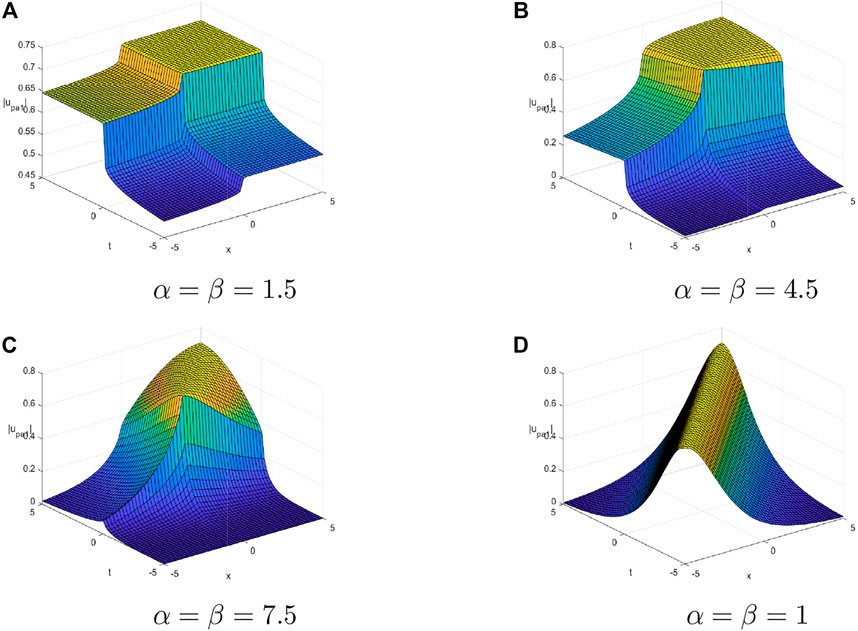
FIGURE 3. 3D plots of bright soliton solutions for the parabolic law non-linearity with the four different fractional values by considering the values A1 = 1, B = −1, v = 1, κ = −1, ω = 3, and δ = 1. (A) α = β = 1.5. (B) α = β = 4.5. (C) α = β = 7.5. (D) α = β = 1.
To solve the dark solitons, starting the hypothesis [43]
where Al and Bl represent the free parameters. Substituting Eq. 82 into Eq. 26, we obtain
The linearly independent function requires the third-order dispersion value to be zero. In addition,
Take Al > 0, and the linearly independent function gives the soliton velocity v, as shown in Eq. 24, and gives the constraint condition Eq. 22. For l = 1, 2, substituting Eq. 82 into Eq. 72, we get
The equilibrium principle gives
The other parameter values from Eq. 85 are
and
The relation is obtained by equalizing the two values of the velocity
Eqs 87–89 introduced the condition bκ ≠ 1 and
Dark soliton solutions for the parabolic law non-linearity are
Figure 4 shows dark soliton solutions for parabolic law non-linearity with the four different fractional values.
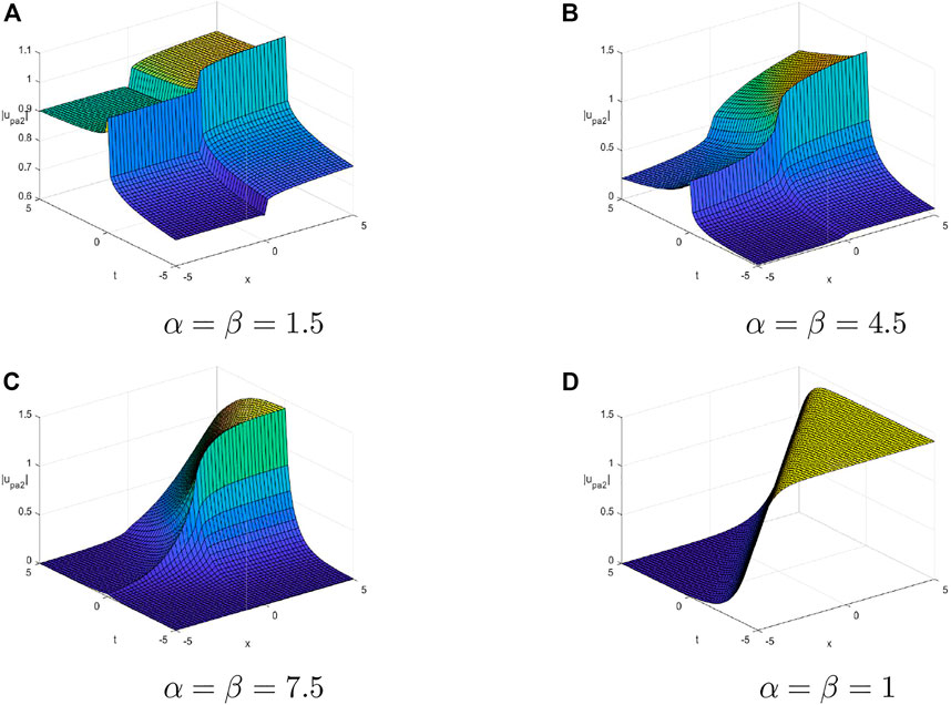
FIGURE 4. 3D plots of dark soliton solutions for the parabolic law non-linearity with the four different fractional values by considering the values A1 = 1, B = −1, v = 1, κ = −1, ω = 3, and δ = 1. (A) α = β = 1.5. (B) α = β = 4.5. (C) α = β = 7.5. (D) α = β = 1.
To solve the singular solitons, starting with the assumption [36]
Combining Eq. 26 with Eq. 93, we get
with the constraint relation bκ ≠ 1.
From the real part, substituting Eq. 93 into Eq. 72, we get
The value of pl with l = 1, 2 is consistent in Eq. 75. According to Eq. 95, linearly independent functions with zero coefficients can get ω, B, and Dl consistent with the parameters given by Eqs 76–78. The corresponding constraints 79, 80 and bκ ≠ 1 still exist. Thus, the parabolic non-linear singular soliton solutions are obtained as
The dual-power law is applied to reveal the saturation in the non-linear refractive index. It is a description of the soliton dynamics in photoelectric photorefractive substances, for example, LiNbO3. For the dual-power law non-linear F(s) = k1sn + k2s2n, Eq. 15 describing the propagation of dispersive solitons can be rewritten as
Substituting the same hypothesis as in Eq. 17 into Eq. 97 and converting to real and imaginary terms, we can get the same imaginary part of Eq. 20. Therefore, the results for this subsection will be the same as Eqs 21–26 for the Kerr law non-linearity as well. The equation for the real part is
Substituting Eq. 73 into Eq. 98, we get
Similarly, based on the equilibrium principle, equating the exponents
From Eq. 99, the coefficients are set to zero, and we get
and
When bκ ≠ 1, other constraint conditions are
and
Bright soliton solutions of the dual-power law non-linearity for the generalized coupled fractional NLS equations (Eq. 97) are
Substituting Eq. 82 into Eq. 98, we get
Similarly, based on the equilibrium principle, equating the exponents (2npl + 2 = 3) gives
From Eq. 107, letting the coefficients to zero yields
where other constraint conditions are bκ ≠ 1 and Eqs 84–91.
Dark soliton solutions for the dual-power law non-linearity are
Substituting Eq. 93 into Eq. 98 yields
Singular soliton solutions for the dual-power law non-linearity of the coupled fractional NLS equations Eq. 97 are
There is no radiation in the case of log law non-linearity, that is to say, there is no energy loss, so it is the optimal mode of soliton communication. c is a constant in the log law non-linearity F(s) = c ln(s). Eq. 12, which describes the propagation of dispersion solitons, is rewritten as
Substitute the same hypothesis in Eq. 17 into Eq. 114 and convert it into real and imaginary numbers to obtain the same imaginary number as Eq. 20. The results of this section are the same as Kerr law non-linearity (Eqs 24–26). The real equation is
Since it is debatable whether the log law non-linearity supports dark solitons or singular solitons, only bright solitons (or Gaussian) can be used for log law.
To solve the bright solitons, form the assumption
Substituting Eq. 116 into Eq. 115 yields
Letting the coefficients of the linearly independent functions τ2j to zero with j = 0, 1, we get
and
Uncoupling Eqs 24, 118, we get
and
When bκ ≠ 1, constraint conditions are
and
Hence, the bright soliton solutions of the log law non-linearity for the generalized coupled fractional NLS equations are
In this paper, the generalized coupled space–time fractional NLS equations are constructed by the semi-inverse method and the Agrawal’s method. In the presence of spatio-temporal dispersion and birefringence, the Kerr, power, parabolic, dual-power, and log law non-linearity laws are studied. Then, we used the ansatz method to obtain the bright, dark, and singular soliton solution of the equations. At the same time, the constraints on the existence of these solitons are given. They can be further extended to other non-linear laws, such as the anti-cubic law, quadratic cubic laws, and cubic power law non-linearity.
The original contributions presented in the study are included in the article/supplementary material; further inquiries can be directed to the corresponding author.
LF: investigation, methodology, writing—original draft, and writing—review and editing. JL: investigation, visualization, and resources. HY: conceptualization, investigation, methodology, and writing—review and editing. HD: investigation and result analysis. XH: investigation, supervision, methodology, validation, and writing—review and editing.
The authors declare that the research was conducted in the absence of any commercial or financial relationships that could be construed as a potential conflict of interest.
All claims expressed in this article are solely those of the authors and do not necessarily represent those of their affiliated organizations, or those of the publisher, the editors, and the reviewers. Any product that may be evaluated in this article, or claim that may be made by its manufacturer, is not guaranteed or endorsed by the publisher.
2. Ferreira MF, Facao MV, Latas SV, Sousa MH. Optical solitons in fibers for communication systems. Fiber Integrated Opt (2005) 24(3-4):287–313. doi:10.1080/01468030590923019
3. Patel MG, Khant SB. Soliton transmission in fiber optics for long distance communication. Int Jounal Adv Res Electr Electron Instrumentation Eng (2014) 3(2):7100–7107.
4. Chakraborty S, Nandy S, Barthakur A. Bilinearization of the generalized coupled nonlinear Schrödinger equation with variable coefficients and gain and dark-bright pair soliton solutions. Phys Rev E (2015) 91(2):023210. doi:10.1103/physreve.91.023210
5. Wazwaz AM, El-Tantawy SA. Gaussian soliton solutions to a variety of nonlinear logarithmic Schrödinger equation. J Electromagn Waves Appl (2016) 30(14):1909–17. doi:10.1080/09205071.2016.1222312
6. Triki H, Wazwaz AM. Soliton solutions of the cubic-quintic nonlinear Schrödinger equation with variable coefficients. Rom J Phys (2016) 61:360366.
7. Chen M, Li B, Yu YX. Darboux transformations, higher-order rational solitons and rogue wave solutions for a (2+1)-dimensional nonlinear Schrödinger equation. Commun Theor Phys (2019) 71(1):027–36. doi:10.1088/0253-6102/71/1/27
8. Wang MM, Chen Y. Dynamic behaviors of general N-solitons for the nonlocal generalized nonlinear Schrödinger equation. Nonlinear Dyn (2021) 104:2621–38. doi:10.1007/s11071-021-06421-3
9. Taghizadeh N, Mirzazadeh M, Frarhrooz F. Exact solutions of the nonlinear Schrödinger equation by the first integral method. Joural Math Anal Appl (2011) 374:549–53. doi:10.1016/j.jmaa.2010.08.050
10. Aktosun T, Busse T, Demontis F, Mee C. Exact solutions to the nonlinear Schrödinger equation. J Phys A: Math Theor (2010) 43(2):1–14. doi:10.1007/978-3-0346-0161-0_1
11. Feng BF, Ling L, Takahashi DA. Multi-breather and high-order rogue waves for the nonlinear Schrödinger equation on the elliptic function background. Stud Appl Math (2020) 144(1):46–101. doi:10.1111/sapm.12287
12. Wang DS, Wang XL. Long-time asymptotics and the bright N-soliton solutions of the Kundu–Eckhaus equation via the Riemann–Hilbert approach. Nonlinear Anal Real World Appl (2018) 41:334–61. doi:10.1016/j.nonrwa.2017.10.014
13. Nonlaopon K, Kumar S, Rezaei S, Bayones FS, Elagan SK. Some optical solutions to the higher-order nonlinear Schrödinger equation with Kerr nonlinearity and a local fractional derivative. Results Phys (2022) 36:105430. doi:10.1016/j.rinp.2022.105430
14. Sun WR, Tian B, Wang YF, Zhen HL. Soliton excitations and interaction for the three-coupled fourth-order nonlinear Schrödinger equations in the alpha helical proteins. Eur Phys J D (2015) 69(146):1–9. doi:10.1140/epjd/e2015-60027-6
15. Kanna T, Lakshmanan M. Exact soliton solutions of coupled nonlinear schrödinger equations: Shape-changing collisions, logic gates, and partially coherent solitons. Phys Rev E (2003) 67(4):046617–2. doi:10.1103/physreve.67.046617
16. West B, Bologna M, Grigolini P. Physics of fractal operators. San Diego: Institute for Nonlinear Science (2003).
17. Tarasov VE. Fractional hydrodynamic equations for fractal media. Ann Phys (2005) 318:286–307. doi:10.1016/j.aop.2005.01.004
18. Baskin E, Iomin A. Electrostatics in fractal geometry: Fractional calculus approach. Chaos, Solitons and Fractals (2011) 44:335–41. doi:10.1016/j.chaos.2011.03.002
19. Tarasov VE. Fractional fokker-planck equation for fractal media. Chaos: Interdiscip J Nonlinear Sci (2005) 15:023102. doi:10.1063/1.1886325
20. Carpinteri A, Cornetti P. A fractional calculus approach to the description of stress and strain localization in fractal media. Chaos, Solitons and Fractals (2002) 13:85–94. doi:10.1016/s0960-0779(00)00238-1
21. Tarasov VE. Fractional dynamics: Applications of fractional calculus to dynamics of particles, fields and media. Beijing: Higher Education Press (2010).
22. Savescu M, Bhrawy A, Hilal E, Alshaery A, Biswas A. Optical solitons in magneto-optic waveguides with spatio-temporal dispersion. Frequenz (2014) 68:445–451. doi:10.1515/freq-2013-0164
23. Younas U, Younis M, Seadawy AR, Rizvi STR, Althobaiti S, Sayed S. Diverse exact solutions for modified nonlinear Schrödinger equation with conformable fractional derivative. Results Phys (2021) 20:103766–10. doi:10.1016/j.rinp.2020.103766
24. Laskin N. Fractional quantum mechanics and Lévy path integrals. Phys Lett A (2000) 268:298–305. doi:10.1016/s0375-9601(00)00201-2
25. Laskin N. Fractional quantum mechanics. Phys Rev E (2000) 62:3135–45. doi:10.1103/physreve.62.3135
26. Laskin N. Fractional schrödinger equation. Phys Rev E (2002) 66:056108. doi:10.1103/physreve.66.056108
27. Herrmann R. Fractional calculus: An introduction for physicists. Singapore: World Scientific (2001).
28. Longhi S. Fractional Schrödinger equationin optics. Opt Lett (2015) 40:1117–1120. doi:10.1364/ol.40.001117
29. Wang FZ, Salama SA, Khater MA. Optical wave solutions of perturbed time-fractional nonlinear Schrödinger equation. J Ocean Eng Sci (2022). doi:10.1016/j.joes.2022.03.014
30. Okposoa NI, Veereshab P, Okposo EN. Solutions for time-fractional coupled nonlinear Schrödinger equations arising in optical solitons. Chin J Phys (2022) 77:965–84. doi:10.1016/j.cjph.2021.10.014
31. Han TY, Li Z, Zhang X. Bifurcation and new exact traveling wave solutions to time-space coupled fractional nonlinear Schrödinger equation. Phys Lett A (2021) 395:127217. doi:10.1016/j.physleta.2021.127217
32. Agrawal OP. Formulation of Euler–Lagrange equations for fractional variational problems. J Math Anal Appl (2002) 272:368–79. doi:10.1016/s0022-247x(02)00180-4
33. Agrawal OP. A general formulation and solution scheme for fractional optimal control problems. Nonlinear Dyn (2004) 38:323–37. doi:10.1007/s11071-004-3764-6
34. Bhrawy A, Alshaery A, Hilal E, Savescu M, Milovic D, Khan KR, et al. Optical solitons in birefringent fibers with spatio-temporal dispersion. Optik-international J Light Electron Opt (2014) 125:4935–44. doi:10.1016/j.ijleo.2014.04.025
35. Vega-Guzman J, Ullah MZ, Asma M, Zhou Q, Biswas A. Dispersive solitons in magneto-optic waveguides. Superlattices and Microstructures (2017) 103:161–70. doi:10.1016/j.spmi.2017.01.020
36. Savescu M, Khan KR, Kohl RW, Moraru L, Yildirim A, Biswas A. Optical soliton perturbation with improved nonlinear Schrödinger’s equation in nano fibers. J Nanoelectronics Optoelectronics (2013) 8:208–20. doi:10.1166/jno.2013.1459
37. Biswas A, Milovic D. Bright and dark solitons of the generalized nonlinear Schrödinger’s equation. Commun Nonlinear Sci Numer Simulation (2010) 15:1473–84. doi:10.1016/j.cnsns.2009.06.017
38. Biswas A, Khan KR, Rahman A, Yildirim A, Hayat T, Aldossary OM. Bright and dark optical solitons in birefringent fibers with Hamiltonian perturbations and kerr law nonlinearity. J Optoelectronics Adv Mater (2012) 14:571.
39. Jumarie G. Table of some basic fractional calculus formulae derived from a modified Riemann–Liouville derivative for non-differentiable functions. Appl Math Lett (2009) 22:378–85. doi:10.1016/j.aml.2008.06.003
40. Gazizov R, Kasatkin A, Lukashchuk SY. Continuous transformation groups of fractional differential equations. Vestnik Usatu (2007) 9:21.
41. Jaradat H. New solitary wave and multiple soliton solutions for the time-space fractional boussinesq equation. Ltalian J Pure Appl Math (2016) 36:367–376.
42. Biswas A, Konar S. Introduction to non-Kerr law optical solitons. Boca Raton: Chapman and Hall/CRC (2006).
Keywords: coupled NLS equations, space–time fractional, optical solitons, birefringent fibers, soliton solutions
Citation: Fu L, Li J, Yang H, Dong H and Han X (2023) Optical solitons in birefringent fibers with the generalized coupled space–time fractional non-linear Schrödinger equations. Front. Phys. 11:1108505. doi: 10.3389/fphy.2023.1108505
Received: 26 November 2022; Accepted: 13 January 2023;
Published: 06 February 2023.
Edited by:
Yunqing Yang, Zhejiang Ocean University, ChinaReviewed by:
Xiangpeng Xin, Liaocheng University, ChinaCopyright © 2023 Fu, Li, Yang, Dong and Han. This is an open-access article distributed under the terms of the Creative Commons Attribution License (CC BY). The use, distribution or reproduction in other forums is permitted, provided the original author(s) and the copyright owner(s) are credited and that the original publication in this journal is cited, in accordance with accepted academic practice. No use, distribution or reproduction is permitted which does not comply with these terms.
*Correspondence: Xiaofeng Han, aGFueGlhb2ZlbmdAc2R1c3QuZWR1LmNu
Disclaimer: All claims expressed in this article are solely those of the authors and do not necessarily represent those of their affiliated organizations, or those of the publisher, the editors and the reviewers. Any product that may be evaluated in this article or claim that may be made by its manufacturer is not guaranteed or endorsed by the publisher.
Research integrity at Frontiers
Learn more about the work of our research integrity team to safeguard the quality of each article we publish.