- 1Center for Advanced Laser Technology, Hebei University of Technology, Tianjin, China
- 2Hebei Key Laboratory of Advanced Laser Technology and Equipment, Tianjin, China
LIDAR is an excellent means to obtain the information of buildings, forests, bridges, tunnels and many other big scenes, but the high price of 3D LIDAR currently limits its further application. To meet this challenge a mobile 3D imaging system based on 2D LIDAR is proposed. The system has the characteristics of large imaging range and low cost. The composition and implementation principle of each module of the system are introduced in detail and a calibration method for the 3-axis assembly error is proposed. In this method Levenberg-Marquardt (LM) optimization algorithm is used to obtain the optimal value of the 2D LIDAR 3-axis attitude angle, which is used to compensate for the point cloud distortion caused by the assembly error. The experimental results show that the proposed method can effectively reduce the point cloud distortion caused by assembly error. This system can meet the application demand of big scenes 3D imaging.
Introduction
3D imaging technology can accurately obtain environmental digital information, and is also the key to realize the “digital twin” technology [1]. Indoor buildings such as rooms and tunnels are essential parts of human life, and these environments have rich structural features. 3D reconstruction of the interior of such buildings can achieve geometric parameter measurement, facilitate monitoring and evaluation of static and dynamic assets to achieve optimal decision-making, such as providing environmental data support for VR, AR and mobile robot navigation.
As a kind of high-precision active detection technology with high resolution and strong anti-interference capability, LIDAR [2] has received wide attention from researchers, which is widely used in autonomous driving [3], remote sensing [4] and 3D reconstruction [5]. 3D LIDAR is certainly capable of 3D detection, but the current high price leads to its poor cost-performance radio in some specific applications. While 2D LIDAR [6] is inexpensive and has achieved more mature commercialization, it is widely used in simultaneous localization and mapping (SLAM) [7] for mobile robots. Compared to 3D LIDAR, 2D LIDAR has higher cost-performance and a more flexible field of view [8], but it can only obtain 2D plane information. If 3D information can be obtained by combining another dimension movement of 2D LIDAR, such a scheme will be more competitive.
At present, the widely used method is to combine 2D LIDAR with a rotating device [9, 10] such as a Pan-Tilt Unit to achieve low-cost 3D scanning of the environment by supplementing the third dimension with rotational scanning of the device. Although such solutions can achieve 3D scanning of the environment, these solutions have the disadvantage of poor detection range. Considering that the actual working environment may be complex or narrow scenes (e.g., offices and hallways), there may also be some obstacles and other objects in the environment. Thus there will be problems such as occlusion, resulting in partial absence of the point cloud, making it difficult to achieve a complete image of the environment in one scan. The device must be moved at multiple locations for multiple scans. The complete point cloud can only be formed after registration at a later stage. So we can see that such operation is complicated, inefficient and may generates registration errors.
Two key points [11] need to be solved in the scheme using 2D LIDAR as the core sensor: one is to reduce the point cloud distortion due to the assembly error [12], and the other is to carry out accurate motion estimation of the device during scanning. Inaccurate motion estimation and assembly errors of the attitude angle will lead to significant point cloud deformation, resulting in global point cloud images unusable.
In view of the characteristics and shortcomings of the above methods, a low-cost 3D imaging system based on 2D LIDAR is proposed in this paper. The 2D LIDAR is mounted vertically on the mobile platform. The scanning plane of the 2D LIDAR is perpendicular to the horizontal plane, and the range data of the vertically mounted 2D LIDAR is combined with the movement data of the mobile platform. When the scanning plane sweeps across a volume in space, the 3D scene information is obtained. This solution overcomes the scanning range of the fixed device and is capable of large-scale scanning task. In this paper, we propose the composition of each module of the system, the implementation principle, and the calibration method for the 3-axis attitude angle. Various experiments are performed to test the superior performance of the system. The experiment results show that point cloud distortion caused by the assembly error of the system is significantly improved and can be used in the measurement of regions and in the complete scene reconstruction.
The remainder of this paper is organized as follows: the components and parameters of the 3D imaging system are described in Section 2, the working principle of the system including the transformation relations between coordinate systems, and the mathematical model for motion estimation, are described in Section 3, Section 4 focuses on the calibration method of the 3-axis attitude angle and revises the complete coordinate generation formula after calibration, Section 5 presents our experimental validation in different scenes to verify the excellent performance of our system. Finally, the summary of our work is outlined in Section 6.
System overview
Hardware system
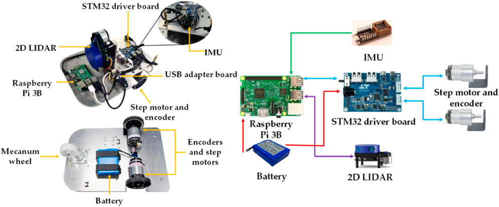
The whole hardware structure of the system is shown in Figure 1. The hardware consists of 2D LIDAR, step motors, IMU, STM32 driver board, Raspberry Pi 3B and power supply. The 2D LIDAR is installed vertically on the center of the mobile platform. The step motors are controlled by STM32 driver board The speed of step motors is read by its optical encoder. The speed is used to achieve wheel odometer. 2D LIDAR, step motors, IMU obtain 2D point cloud, speed and attitude angle respectively. The obtained information is transmitted to Raspberry Pi 3B, and fused to generate the whole 3D point cloud by multi-sensor fusion algorithm.
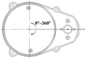
The 2D LIDAR we use in this study is YDLIDAR X4, this sensor is based on the laser triangulation principle. The built-in rotating module drives the ranging module to rotate 360° to achieve 360° rotational scan, then the sampled laser points information of the ranging distance and its scanning angle can be obtained. The definition of the scanning angle is shown in Figure 2. The scanning angle is the angle between the laser measurement optical path and the vertical direction. The specific parameters are shown in Table 1. It has high cost-performance and can meet the performance requirements of general indoor applications. The IMU is HI 219, and its specific accuracy is shown in Table 2. The speed accuracy of the step motors is 1% per meter.
Software system
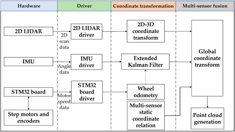
Our software system is based on Robot Operating System (ROS), and the software system is divided into three levels, namely, hardware driver, coordinate transformation, and multi-sensor fusion. The software architecture is shown in Figure 3.
The hardware driver is responsible for controlling and reading the range data from 2D LIDAR, pose data from IMU, and sending velocity control commands to the STM32 driver board. And the driver board controls the motor speed through PID algorithm and receives motor velocity which is transmitted back to Raspberry Pi for motion estimation of the wheel odometer. The relative position of each sensor is defined in the coordinate transformation module. And the coordinate transformation module is also responsible for fusing the pose data from IMU and the wheel odometer to complete motion estimation of the platform by Extended Kalman Filter (EKF). The data fusion module fuses the transformation matrix obtained from the motion estimation and the range data from 2D LIDAR to generate the coordinates in the world coordinate system. The complete point cloud is generated by adding up the coordinates in the world coordinate system frame by frame.
Operation principle
Coordinate system model
In this section we define the coordinate systems of multiple sensors in the system, and the coordinate systems are all in Cartesian right-handed coordinate system. The transformation relationship between the coordinate systems is elaborated.
As shown in Figure 4, we define Body as the center of motion, Laser as the coordinate system of 2D LIDAR, and Imu as the coordinate system of IMU. The coordinate system Body is used as the origin to establish the reference coordinate system. The world coordinate system is the geodetic coordinate system, which coincides with the initial position of the Body coordinate system. As shown in Figure 4, h is the distance from the origin of the 2D LIDAR coordinate system to the xOy plane of the reference coordinate system, wheel_distance is the distance from the center of the wheel to the center of motion, l1 is the displacement from the center of the 2D LIDAR coordinate system to the reference coordinate system along the x-axis direction, and l2 is the displacement from the center of the IMU coordinate system to the reference coordinate system along the x-axis direction. A 2D point in the lidar frame is obtained by converting a range measurement ρ from polar to Cartesian coordinate using the current position of the lidar rotating angle θ in Eq. 1.
Wheel odometer
The motion of the platform can be regarded as the rigid body plane motion, which can be decomposed into two kinds of motion: translation and rotation, which contains the translation in x-y direction, and the rotation around z-axis. So the motion of the platform can be decomposed into 3 degrees of freedom. When the speed of the left and right driving wheels are the same, the position of the platform changes and the heading direction remains the same, while different, the position and the heading direction both change at the same time. We use the optical encoder on the driving wheels to read the rotational speed of the left and right driving wheels. The wheel odometer model is established based on the rotational speed of the two wheels, respectively.
The velocity of the geometric center is [vc ω]T. The linear velocity vc is positive when the heading direction is the same as the x-axis direction, and negative when opposite; the angular velocity ω is positive when the car rotates counterclockwise, and negative when opposite.
Then we have the kinematic recurrence relation matrix
Where
Extended kalman filter
Since wheel slippage is inevitable, using the wheel odometer model alone for track deduction will result in errors, leading to inaccurate motion estimation. To obtain more accurate motion estimation, we use an EKF to fuse the wheel odometer and IMU.
Extended Kalman Filter is divided into two parts: prediction and update.
The complete state variables of the platform are defined as
The equation of state of the system is defined as:
Then the system state transfer equation is defined as:
Where
Where
1) Prediction. Calculate the predicted value
2) Update. Calculate Kalman gain, optimal estimate and error covariance matrix:
In this section we define the coordinate systems of multiple sensors in the system, and the coordinate systems are all in Cartesian right-handed coordinate system. The transformation relationship between the coordinate systems is elaborated.Where Hk is the Jacobi matrix of the sensor function and Rk is the variance of the normal distribution at moment k.
Extended Kalman Filter can get more accurate coordinates of the car in the world coordinate system. So the transformation matrix from the reference coordinates to world coordinates can be obtained as follows
Then we can obtain the global point cloud coordinate equation.
Calibration method and strategy
Calibration method
The quality of the point cloud depends on the accuracy of its coordinates which are obtained by the precise transformation matrix between coordinate systems [13]. Since assembly errors will inevitably exist during assembly, it is not physically possible to install the 2D LIDAR perfectly vertically. So angular deviations will inevitably occur, that is, the actual 2D LIDAR coordinate system L′ may not coincide with the theoretical coordinate system L. The bias includes three rotational degrees of freedom (coordinate system rotational angle γ along the x-axis, angle β along the y-axis, angle α along the z-axis), which will result in the ideal scanning plane being different from the actual, as shown in Figure 5.

FIGURE 5. The comparison of the ideal and actual laser scanning plane due to the angular error about the three axes (A) x-axis (B) y-axis (C) z-axis.
Therefore, the bias will cause the actual rotation matrix to be different from the theoretical rotation matrix, which in turn will lead to distortions in the global point cloud. When the car drives along a complete circle, the certain object will be repeatedly scanned twice and this distortion becomes a particularly noticeable ghost image, as shown in Figure 6. We can find distortion between two parts of the ceiling and the vertical wall after two scans.
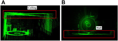
FIGURE 6. Original scan captured by our system without calibration, visible distortion is marked in red box (A) distortion in ceiling (B) distortion in wall.
Therefore, it is necessary to calibrate the three-axis attitude angle of the 2D LIDAR accurately to obtain the accurate transformation matrix between the actual and ideal coordinate systems. The traditional measurement-based methods are difficult to obtain accurate calibration results, so after the equipment is built, real point cloud need to be collected for calibration. Some calibration methods have been proposed for such problems. The methods provided in the literature [14–16] require the addition of camera and checkerboard, etc. For calibration, which is complex to operate and the added sensors may introduce more uncertainties. The method provided in the literature [17] calibrate only one angle rather than three, so the final result still has some errors. The calibration method based on planar alignment proposed in this paper is able to perform a complete calibration of the three-axis attitude angle without adding another sensor, and obtain an accurate three-axis attitude angle.
The rotation matrix of the 2D LIDAR is defined as
So the complete coordinate transformation is defined correctly as
Calibration is carried out according to the following steps:
1) Actuate the car to drive along a circle at a constant rate;
2) Extract the calibration target and determine the corresponding points, establish the cost function;
3) Calculate the three-axis attitude angle when the cost function is minimized using the LM nonlinear optimization algorithm;
4) Adjust the transformation matrix according to the calibration results and regenerate the point cloud;
5) Fit the ceiling plane using the RANSAC algorithm and analyze the fitting effect.
The calibration target is stuck on the window so that it is convenient to extract the target plane. When the car is actuated according to the above steps, and the point cloud of the calibration target can be obtained after two scans. As the car drives along a circle at a constant rate, the calibration target is actually scanned twice, which can be used to construct two point clouds. However, the corresponding points of the two scans cannot be overlapped due to the bias of the 2D LIDAR, as shown in Figure 7.
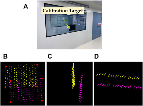
FIGURE 7. Experiment environment and different views of the point cloud obtained by two scans of the calibration target (A) experiment environment (B) front view (C) side view (D) top view.
LM Optimized Algorithm.
We define the distance between the corresponding laser points in the two point clouds as
Where
Where the cost function is defined as
Four corresponding edge points are selected in each scan, as shown in Figure 7B. The selected four matching pairs of points are used in Equation 17 to obtain the optimal calibration parameters. The calibration problem is a nonlinear optimization problem, and we apply the LM algorithm to solve it.
Experiments and analysis
After the establishment of system and the calibration model, we performed the calibration experiment and scanning experiment in practical indoor environment, and analyzed the measurement accuracy of the system respectively.
Calibration experiment
In the calibration experiment, we actuate the car according to the steps mentioned in Section 4, the radius of the driving circle of the center of motion is 0.83 m, and the calibration target is placed in the environment, as shown in Figure 7A. The LM algorithm is used to optimize the calibration formula, and the mean square error variation curve of the point cloud and the variation curve of the three-axis attitude angle with the number of iterations during the iteration are shown in Figure 8.
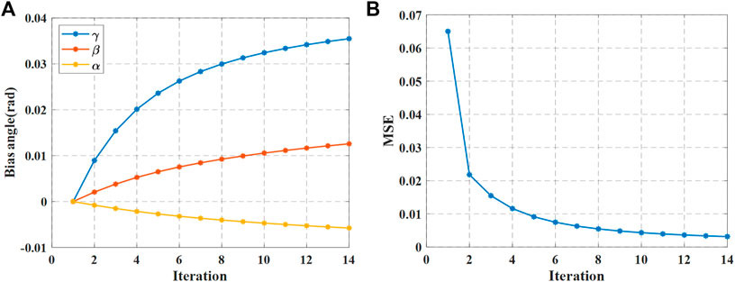
FIGURE 8. LM algorithm optimization results of calibration (A) optimization results of three-axis attitude Angle under different iterations (B) MSE of two point clouds.
After adopting LM algorithm, the final result is α = -0.0058 rad, β = 0.0126 rad, γ = 0.0355 rad. We use the calibration results into Equation 14 to reconstruct the point cloud. As shown in Figures 9A,B, the distortion of the ceiling and wall has been improved significantly. To characterize the accuracy of the calibration, we calculate the deviation and normal vector between the measured plane and the actual plane to evaluate the accuracy of our method, where the plane normal vector is obtained by plane fitting using RANSAC algorithm, and the obtained normal vector is (-0.012,0.011,0.099)T, which is very close to (0,0,1)T. As shown in Figure 9C D, the deviation comparison of calibrated and uncalibrated plane is visualized by histogram.
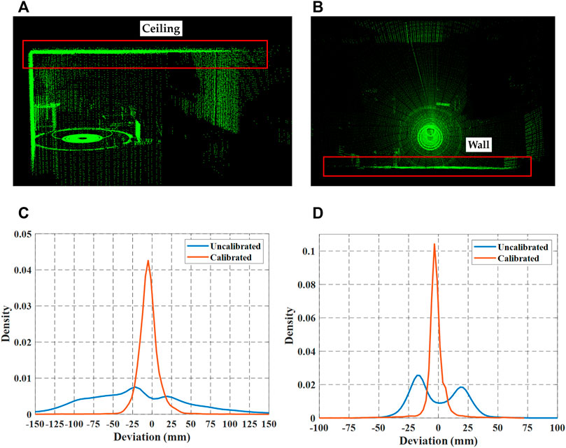
FIGURE 9. Deviation comparison of the uncalibrated plane and the calibrated plane, respectively (A) ceiling plane (B) wall plane (C) ceiling plane histogram (D) wall plane histogram.
Similarly, we performed a comparison test in a stairwell, an environment with more structured scenes for observing the aberrations. We controlled the car to scan a specific area twice and calibrated the point cloud distortion according to the optimal value in Section 5.1. By comparing the point clouds obtained before and after calibration, we can see that the distortion of the point cloud has improved significantly. The results of the test are shown in Figure 10.
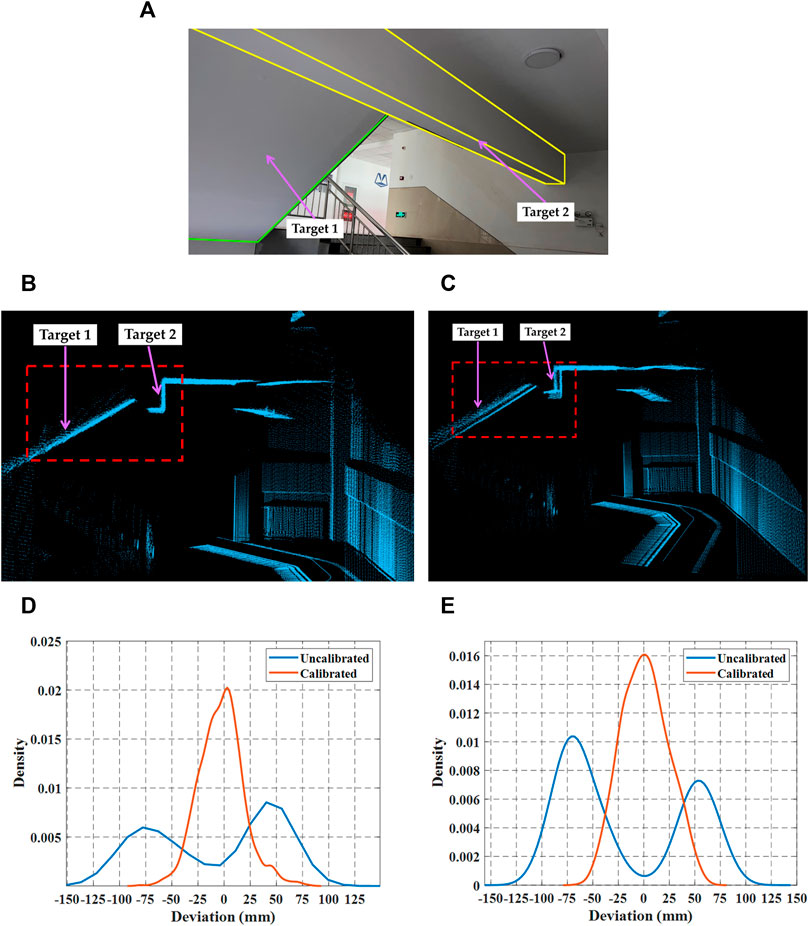
FIGURE 10. Deviation comparisons in a stairwell. The ladder plate and platform beam are used as the contrast objects, namely, Target one and Target 2 (A) the experiment scene: stairwell (B) target point cloud before calibration (C) target point cloud after calibration (D) deviation comparison of Target 1 (E) deviation comparison of Target 2.
Scanning experiment
We performed a complete scan of the laboratory, tested the good performance of Extended Kalman Filter, point cloud density and measurement accuracy. The environment is a 10*5*2.5 m room, the car drives in a closed loop, moving at a speed about 0.20 m/s. The experiment scene and results are shown in Figure 11. Due to the wheel odometer’s error, the trajectory is inaccurate and the loop cannot be closed. During the scanning process, some areas were scanned twice and we can see some mismatch in those areas. As shown in Figures 11C,D, we can see some details in the zoomed-in region, which shows the improvement of the EKF optimization. After the application of EKF optimization, the trajectory is more accurate, so the mismatch of the point cloud is significantly improved. As shown in Figures 11E,F, some objects in the lab can be displayed in the point cloud, but some objects cannot due to the different scattering and absorption of the laser by the object material.
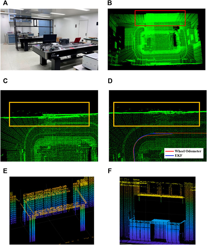
FIGURE 11. Different views of the point cloud (A) the experiment environment (B) top view of the point cloud (C) the mismatch before EKF optimization (D) the mismatch after EKF optimization (E) worktop (F) laboratory casework.
We used a representation based on the average distance to represent the sparsity of the point cloud distribution. In a point cloud C with number of points N, dis(p,q) denotes the distance between point p and any other point q, and
Where
The smaller the
In order to evaluate the measurement accuracy of the system, we first filter the point cloud to reduce noise, and then use RANSAC algorithm to fit different wall and ceiling planes to obtain the plane equations of the corresponding planes, as shown in Figure 12A. The fitting results are listed in Equations 20–24. Then, we use the distance of the corresponding plane to represent the experimental value of
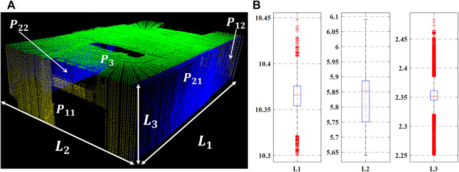
FIGURE 12. Accuracy results (A) plane segmentation results (B) measurement statistical results shown in boxplots.
The comparison of experimental and actual value is shown in Table 3. From the results, we can see that the accuracy of the system is acceptable.
Conclusion
In summary, this paper proposes a low-cost mobile 3D imaging system based on 2D LIDAR. The software and hardware components are introduced, and the theoretical model is derived. The system can realize a wide range of 3D scanning of the environment, which can be used for big scenes 3D mapping and reconstruction. For this system, the assembly error of 2D LIDAR is an important cause of point cloud distortion. To solve this problem, we propose a calibration method based on targeted calibration plane registration, which can calibrate the 3-axis error angles without adding extra sensor. LM nonlinear optimization algorithm is used to calculate the results. The experiments verify the superior performance of the system and the validity of the calibration method. The system not only reduces the cost but also ensures the accuracy. It is anticipated that this system will greatly expand the availability of LIDAR in a wide range of applications.
Data availability statement
The original contributions presented in the study are included in the article/Supplementary Material, further inquiries can be directed to the corresponding author.
Author contributions
Writing-original draft preparation, conceptualization was provided by RM Data curation was provided by XL Investigation, methodology was provided by YP Validation, formal analysis was provided by LL.
Funding
This research was funded by the National Natural Science Foundation of China (NSFC) (61905063, 61905061); the Natural Science Foundation of Hebei Province, China (F2020202055).
Acknowledgments
The authors are thankful to other colleagues in their laboratory for their understanding and help.
Conflict of interest
The authors declare that the research was conducted in the absence of any commercial or financial relationships that could be construed as a potential conflict of interest.
Publisher’s note
All claims expressed in this article are solely those of the authors and do not necessarily represent those of their affiliated organizations, or those of the publisher, the editors and the reviewers. Any product that may be evaluated in this article, or claim that may be made by its manufacturer, is not guaranteed or endorsed by the publisher.
References
1. Baek J, Park J, Cho S, Lee C. 3D global localization in the underground mine environment using mobile LiDAR mapping and point cloud registration. Sensors (2022) 22:2873. doi:10.3390/s22082873
2. Williams K, Olsen MJ, Roe GV, Glennie C. Synthesis of transportation applications of mobile LIDAR. Remote Sensing (2013) 5:4652–92. doi:10.3390/rs5094652
3. Li Y, Ibanez-Guzman J. Lidar for autonomous driving: The principles, challenges, and trends for automotive lidar and perception systems. IEEE Signal Process Mag (2020) 37:50–61. doi:10.1109/msp.2020.2973615
4. Liu K, Ma HC, Ma HC, Cai Z, Zhang L. Building extraction from airborne LiDAR data based on min-cut and improved post-processing. Remote Sensing (2020) 12:2849. doi:10.3390/rs12172849
5. Wu QY, Yang HB, Wei MQ, Remil O, Wang B, Wang J. Automatic 3D reconstruction of electrical substation scene from LiDAR point cloud. ISPRS J Photogrammetry Remote Sensing (2018) 143:57–71. doi:10.1016/j.isprsjprs.2018.04.024
6. Konolige K, Augenbraun J, Donaldson N, Fiebig C, Shah P. Ieee. A low-cost laser distance sensor. In: Proceedings of IEEE international conference on robotics and automation. Pasadena, CA (2008). p. 3002–+. doi:10.1109/ROBOT.2008.4543666
7. Hess W, Kohler D, Rapp H, Andor D. Real-time loop closure in 2D LIDAR SLAM. Ieee Int Conf Robotics Automation (Icra) (2016) 1271–8. doi:10.1109/icra.2016.7487258
8. Wang H, Lin Y, Wang Z, Yao Y, Zhang Y, Wu L. Validation of a low-cost 2D laser scanner in development of a more-affordable mobile terrestrial proximal sensing system for 3D plant structure phenotyping in indoor environment. Comput Elect Agric (2017) 140:180–9. doi:10.1016/j.compag.2017.06.002
9. Xu X, Luo M, Tan Z, Zhang M, Yang H. Plane segmentation and fitting method of point clouds based on improved density clustering algorithm for laser radar. Infrared Phys Tech (2019) 96:133–40. doi:10.1016/j.infrared.2018.11.019
10. Bauersfeld L, Ducard G. Low-cost 3D laser design and evaluation with mapping techniques review. In: Proceedings of 2019 IEEE sensors applications symposium (2019). (SAS).
11. Bi S, Yuan C, Liu C, Cheng J, Wang W, Cai Y. A survey of low-cost 3D laser scanning technology. Appl Sci (2021) 11:3938. doi:10.3390/app11093938
12. Yuan C, Bi S, Cheng J, Yang D, Wang W. Low-cost calibration of matching error between lidar and motor for a rotating 2D lidar. Appl Sci (2021) 11:913. doi:10.3390/app11030913
13. Zhao Haipeng H, Du Yuhong Y, Ding Juan J, Zhao Di D, Shi Yijun Y. LiDAR ranging angle measurement calibration method in mobile robot. 红外与激光工程 (2019) 48(68):630002–0630002. doi:10.3788/irla201948.0630002
14. Olivka P, Krumnikl M, Moravec P, Seidl D. Calibration of short range 2D laser range finder for 3D SLAM usage. J Sensors (2016) 3715129. doi:10.1155/2016/3715129
15. So E, Basso F, Menegatti E. Calibration of a rotating 2D laser range finder using point-plane constraints. J Automation Mobile Robotics Intell Syst (2013). doi:10.1007/978-3-319-10774-5_15
16. Kurnianggoro L, Hoang V, Jo KH. Calibration of a 2D laser scanner system and rotating platform using a point-plane constraint. Comsis J (2015) 12:307–22. doi:10.2298/csis141020093k
Keywords: lidar, 3D imaging, point cloud, calibration, mobile
Citation: Miao R, Liu X, Pang Y and Lang L (2022) Design of a mobile 3D imaging system based on 2D LIDAR and calibration with levenberg–marquardt optimization algorithm. Front. Phys. 10:993297. doi: 10.3389/fphy.2022.993297
Received: 13 July 2022; Accepted: 10 August 2022;
Published: 30 August 2022.
Edited by:
Baitao Zhang, Shandong University, ChinaReviewed by:
Xiaofei Yang, Shanghai Institute of Optics and Fine Mechanics (CAS), ChinaJinbao Xia, Shandong University, China
Copyright © 2022 Miao, Liu, Pang and Lang. This is an open-access article distributed under the terms of the Creative Commons Attribution License (CC BY). The use, distribution or reproduction in other forums is permitted, provided the original author(s) and the copyright owner(s) are credited and that the original publication in this journal is cited, in accordance with accepted academic practice. No use, distribution or reproduction is permitted which does not comply with these terms.
*Correspondence: Yajun Pang, eWpwYW5nQGhlYnV0LmVkdS5jbg==
 Ruikai Miao
 Xinyue Liu1,2
 Yajun Pang