A VTI anisotropic media inversion method based on the exact reflection coefficient equation

Anisotropy is widespread in the Earth’s crust, and VTI (vertical axis symmetry transverse isotropy) anisotropy is common due to stratigraphic pressure. Disregarding anisotropy leads to inaccurate inversion results in VTI media. To estimate accurate elastic parameters, the exact reflection coefficient equation of VTI media should be used. This equation is nonlinear and more accurate than the commonly used linear reflection coefficient equation. Although the inversion based on the VTI anisotropy exact reflection coefficient equation is a complex nonlinear inversion problem, it is still computable. Therefore, for VTI media, we derive the objective function combining Bayesian theory and use the iterative reweighted least squares method for a fast and stable solution. Adding Bayesian theory can improve the robustness of the algorithm. The accuracy and noise immunity of the method is tested with synthetic data. Finally, the method is applied on field data and obtains accurate elastic parameters. The results can provide an understanding of subsurface formations and serve as the base data for calculating fluid and fracture distribution.

Introduction

VTI (vertical axis symmetry transverse isotropy) anisotropy resulting from textured minerals or sequences of horizontal thin layers is one of the most common forms of anisotropy in sedimentary formations [1–3]. In VTI media, a large number of linear approximate reflection coefficient equations are used in AVO (amplitude versus offset) inversion, with underlying assumptions of small incidence angles and weak impedance contrasts limiting the applicability and accuracy of the inversion. The exact VTI reflection coefficient equation can solve these problems well. To address this issue, the inverse problem can be solved with Bayesian theory.

Forward equations are a central ingredient of inversion algorithms, and the relationship between the VTI elastic parameters and the pre-stack seismic records is their cornerstone. The reflection and transmission equation of anisotropic media were first discussed by Henneke [4] and 37. Graebner [5] simplified the form of Daley and Hron’s [6] algebraic equation, and Rüger [7] modified Graebner’s equation. However, the exact form of the reflection coefficient is very complex and it is difficult to account for inversion. Therefore, a large number of approximate equations have been derived and applied. Thomsen [8] derived an approximate expression for the P-wave reflection coefficient based on a linear approximation of the exact VTI reflection coefficient equation with the assumption of weak anisotropy. Rüger [9] modified Thomsen’s equation for the P-wave reflection coefficient to account for a larger range of angles; this approximation is straightforward and therefore often used for AVO/AVA analysis and inversion. To facilitate the joint inversion, Jílek [10] proposed a PS-wave reflection coefficient equation for anisotropic media. Shaw and Sen [11] derived the PP- and PS-wave reflection coefficients for arbitrary weakly anisotropic media using the Born integral. Based on the above linear approximate forward equations, many scholars have implemented inversion calculations. Plessix and Bork [12] analyzed the quantitative estimation of the elastic and anisotropic parameters of VTI media from the pre-stack AVA records based on the linear approximation equation. Zhang et al. [13], based on an improved Rüger approximation equation, simultaneously inverted the gradient, intercept, and P-wave velocity. Zhang and Li [14] derived a VTI media approximate reflection coefficient equation containing the second-order term of the anisotropic parameter and implemented inversion. The results show that the accuracy of the second-order approximation equation is higher than the first-order. Zhang and Li [15] tested the effectiveness of the simultaneous inversion of the elastic and anisotropy parameters method on VTI anisotropic shale formations. However, there is a contradiction: to accurately obtain density and Thomsen anisotropic parameters, large incidence angles (>30°) of seismic records need to be used [12,16]. However, the non-negligible error in the linear reflection coefficient equation at large angles leads to the poor accuracy of the inverse results. There are relatively few studies related to exact VTI reflection coefficient equation inversion. Amit and Subhashis [17] implemented a pre-stack joint inversion based on the exact VTI reflection coefficient equation using a revised genetic algorithm. However, the algorithm is time-consuming and cannot be applied to large-scale work area data.

In summary, considering accuracy and practicality, we derive a VTI media inversion method based on the exact reflection coefficient equation. The algorithm adds constraint by Bayesian theory. The superiority of the method is verified by numerical model testing and real data application.

Theory

Exact reflection coefficient equation for VTI media

The Thomsen anisotropy parameters [18] mainly describe the relationship between two vertical velocities, three dimensionless anisotropy parameters, and five stiffness coefficients based on the weak anisotropy assumption. The relations are as follows:

$V_P=\sqrt{\frac{c_{33}}{\rho }},V_S=\sqrt{\frac{c_{55}}{\rho }},\epsilon =\frac{c_{11}-c_{33}}{2c_{33}},\gamma =\frac{c_{66}-c_{44}}{2c_{55}},\delta =\frac{{\left(c_{13}+c_{55}\right)}^2-{\left(c_{33}-c_{55}\right)}^2}{2c_{33}\left(c_{33}-c_{55}\right)},(1)$

where V_P and V_S denote the P- and S-wave velocity in the vertical direction (symmetry axis direction) respectively, ρ denotes the density, and ε, δ, and γ are the Thomsen anisotropy parameters. Since the SH-wave is completely decoupled from the P- and SV-waves in VTI media, the reflection and transmission coefficients of the P- and SV-waves are considered.

Based on the weak anisotropy assumption, the P-wave phase velocity and stiffness coefficient c₁₃ in the VTI media can be linearly expressed by anisotropy parameters ε and δ as [18]:

$V_P\left(\theta \right)\approx V_{P0}\left(1+\delta {\sin }^2\theta {\cos }^2\theta +\epsilon {\sin }^4\theta \right),(2)$

$c_{13}\approx c_{33}\left(1+\delta \right)-c_{55}.(3)$

According to Eq. 2, a relatively simple form of horizontal slowness (ray parameter) can be obtained:

$p=\frac{\sin \theta }{V_P\left(1+\delta {\sin }^2\theta {\cos }^2\theta +\epsilon {\sin }^4\theta \right)}.(4)$

Substituting Eqs 1, 3 into the VTI media exact reflection coefficient equation [5,7,19], we can give the matrix:

$\left[\begin{array}{cccc}{m}_{11}& m_{12}& m_{13}& m_{14}\\ m_{21}& m_{22}& m_{23}& m_{24}\\ m_{31}& m_{32}& m_{33}& m_{34}\\ m_{41}& m_{42}& m_{43}& m_{44}\end{array}\right]\left[\begin{array}{c}{R}_{PP}^{VTI}\\ R_{PS}^{VTI}\\ T_{PP}^{VTI}\\ T_{PS}^{VTI}\end{array}\right]=\left[\begin{array}{c}-m_{11}\\ -m_{21}\\ m_{31}\\ m_{41}\end{array}\right].(5)$

As with the exact Zoeppritz equation [20,21], Eq. 5 can be expressed in the following form:

$M•S=N.(6)$

In Eq. 5, the coefficients of the matrix are given by:

$\begin{array}{l}{m}_{11}=l_{\alpha }^{\left(1\right)},m_{12}=m_{\beta }^{\left(1\right)},m_{13}=-l_{\alpha }^{\left(2\right)},m_{14}=-m_{\beta }^{\left(2\right)},\\ m_{31}=m_{\alpha }^{\left(1\right)},m_{32}=-l_{\beta }^{\left(1\right)},m_{33}=-m_{\alpha }^{\left(2\right)},m_{34}=-l_{\beta }^{\left(2\right)},\\ m_{21}=p{l}_{\alpha }^{\left(1\right)}\left(\left(1+{\delta }^{\left(1\right)}\right){\rho }^{\left(1\right)}{V_{P0}^2}^{\left(1\right)}-2{\rho }^{\left(1\right)}{V_{S0}^2}^{\left(1\right)}\right)+q_{\alpha }^{\left(1\right)}{m}_{\alpha }^{\left(1\right)}{\rho }^{\left(1\right)}{V_{P0}^2}^{\left(1\right)},\\ m_{22}=p{m}_{\beta }^{\left(1\right)}\left(\left(1+{\delta }^{\left(1\right)}\right){\rho }^{\left(1\right)}{V_{P0}^2}^{\left(1\right)}-2{\rho }^{\left(1\right)}{V_{S0}^2}^{\left(1\right)}\right)-q_{\beta }^{\left(1\right)}{l}_{\beta }^{\left(1\right)}{\rho }^{\left(1\right)}{V_{P0}^2}^{\left(1\right)},\\ m_{23}=-\left(p{l}_{\alpha }^{\left(2\right)}\left(\left(1+{\delta }^{\left(2\right)}\right){\rho }^{\left(2\right)}{V_{P0}^2}^{\left(2\right)}-2{\rho }^{\left(2\right)}{V_{S0}^2}^{\left(2\right)}\right)+q_{\alpha }^{\left(2\right)}{m}_{\alpha }^{\left(2\right)}{\rho }^{\left(2\right)}{V_{P0}^2}^{\left(2\right)}\right),\\ m_{24}=-\left(p{m}_{\beta }^{\left(2\right)}\left(\left(1+{\delta }^{\left(2\right)}\right){\rho }^{\left(2\right)}{V_{P0}^2}^{\left(2\right)}-2{\rho }^{\left(2\right)}{V_{S0}^2}^{\left(2\right)}\right)-q_{\beta }^{\left(2\right)}{m}_{\beta }^{\left(2\right)}{\rho }^{\left(2\right)}{V_{P0}^2}^{\left(2\right)}\right),\\ m_{41}={\rho }^{\left(1\right)}{V_{S0}^2}^{\left(1\right)}\left(q_{\alpha }^{\left(1\right)}{l}_{\alpha }^{\left(1\right)}+p{m}_{\alpha }^{\left(1\right)}\right),m_{42}={\rho }^{\left(1\right)}{V_{S0}^2}^{\left(1\right)}\left(q_{\beta }^{\left(1\right)}{m}_{\beta }^{\left(1\right)}+p{l}_{\beta }^{\left(1\right)}\right),\\ m_{43}={\rho }^{\left(2\right)}{V_{S0}^2}^{\left(2\right)}\left(q_{\alpha }^{\left(2\right)}{l}_{\alpha }^{\left(2\right)}+p{m}_{\alpha }^{\left(2\right)}\right),m_{44}={\rho }^{\left(2\right)}{V_{S0}^2}^{\left(2\right)}\left(q_{\beta }^{\left(2\right)}{m}_{\beta }^{\left(2\right)}+p{l}_{\beta }^{\left(2\right)}\right),\end{array}(7)$

The superscripts ⁽¹⁾ and ⁽²⁾ indicate the upper and lower layer respectively, where:

$\begin{array}{l}{l}_{\alpha }=\sqrt{\frac{V_{P0}^2{q}_{\alpha }^2+V_{S0}^2{p}^2-1}{\left(2\epsilon +1\right)V_{P0}^2{p}^2+V_{S0}^2{q}_{\alpha }^2+V_{P0}^2{q}_{\alpha }^2+V_{S0}^2{p}^2-2}},\\ m_{\alpha }=\sqrt{\frac{V_{S0}^2{q}_{\alpha }^2+\left(2\epsilon +1\right)V_{P0}^2{p}^2-1}{\left(2\epsilon +1\right)V_{P0}^2{p}^2+V_{S0}^2{q}_{\alpha }^2+V_{P0}^2{q}_{\alpha }^2+V_{S0}^2{p}^2-2}},\\ l_{\beta }=\sqrt{\frac{V_{S0}^2{q}_{\beta }^2+\left(2\epsilon +1\right)V_{P0}^2{p}^2-1}{\left(2\epsilon +1\right)V_{P0}^2{p}^2+V_{S0}^2{q}_{\beta }^2+V_{P0}^2{q}_{\beta }^2+V_{S0}^2{p}^2-2}},\\ m_{\beta }=\sqrt{\frac{V_{P0}^2{q}_{\beta }^2+V_{S0}^2{p}^2-1}{\left(2\epsilon +1\right)V_{P0}^2{p}^2+V_{S0}^2{q}_{\beta }^2+V_{P0}^2{q}_{\beta }^2+V_{S0}^2{p}^2-2}}.\end{array}(8)$

In the above equations for the VTI reflection and transmission coefficients, the vertical slowness of the different wave modes can be expressed as [7]:

$\begin{array}{l}{q}_{\alpha }=\frac{\sqrt{K_1-\sqrt{K_1^2-4K_2{K}_3}}}{\sqrt{2}},\\ q_{\beta }=\frac{\sqrt{K_1+\sqrt{K_1^2-4K_2{K}_3}}}{\sqrt{2}},\end{array}(9)$

where:

$\begin{array}{l}{K}_1=\frac{\rho }{c_{33}}+\frac{\rho }{c_{55}}-\left(\frac{c_{11}}{c_{55}}+\frac{c_{55}}{c_{33}}-\frac{{\left(c_{13}+c_{55}\right)}^2}{c_{33}{c}_{55}}\right)p^2,\\ K_2=\frac{c_{11}}{c_{33}}{p}^2-\frac{\rho }{c_{33}},\\ K_3=p^2-\frac{\rho }{c_{55}},\end{array}(10)$

and q_α is the vertical slowness of the P-wave, q_β is the vertical slowness of the SV-wave, c_ij is the stiffness tensor, and θ is the phase angle. Subscripts _α and _β denote the P-wave mode and SV-wave mode, respectively.

Substituting Eqs 1, 3 into Eq. 10 replaced the independent stiffness coefficients with the Thomsen anisotropy parameters.

Eq. 5 is an implicit equation of the VTI media reflection and transmission coefficients. Eqs 4, 7–9 are the intermediate variables of Eq. 5. These equations are combined to form the forward operator.

In order to compare the difference between the exact and linear of approximation reflection coefficient in VTI media, as well as the reflection coefficient of the exact Zoeppritz equation, we solve the forward problem for the elastic parameters provided in Tables 1 and 2. The linear approximation reflection coefficient equation comes from Rüger [9].

TABLE 1

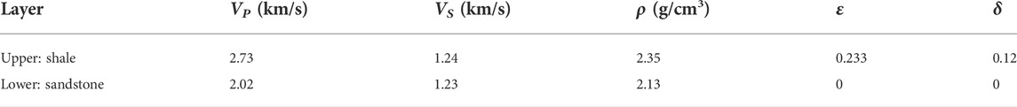
TABLE 1. Model parameters: the VTI/isotropy interface from Rüger [7].

TABLE 2

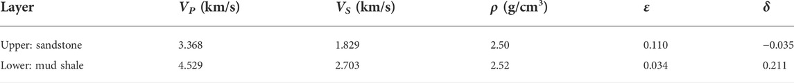
TABLE 2. Model parameters: the VTI/VTI interface from Thomsen [18].

Figure 1 shows the results for P-wave incidence angles of 0°–60°. As shown from the figure, although the approximation still predicts the correct trend at a lower incidence angle, the gap between the three curves becomes larger as the angle increases. The behavior of the reflection coefficient curves is substantially different, including their slopes (or AVO gradient)—especially in higher incidence angles.

FIGURE 1

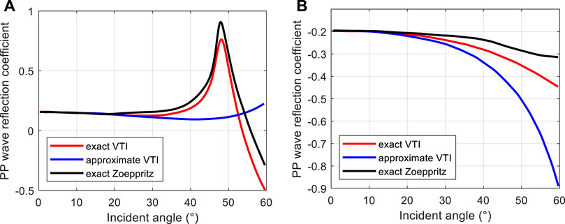
FIGURE 1. Comparison of the exact VTI reflection coefficient equations (red), linear equation (blue), and exact Zoeppritz reflection coefficient equations (black). (A) VTI/VTI interface; (B) VTI/isotropic interface.

Anisotropy mainly affects the velocity, which in turn affects the reflection coefficient. Therefore, the reflection coefficient curves of isotropic and anisotropic media are different. The approximate reflection coefficient equation has the assumption of a small incidence angle. As seen in Figure 1, the area of application of the approximate reflection coefficient equation is the incidence angle <30°. The difference between the exact and approximate curve increases with the increase of the incidence angle. In summary, for anisotropic strata, which are widely present in the upper crust, it is accurate to use the anisotropic exact reflection coefficient equation for forward/inverse problems.

Constructing objective function based on Bayesian theory

Forward modeling can be written in the classical form of d = Gm + n, where G is a nonlinear forward operator and n is the noise in the observed seismic records. In pre-stack seismic inversion, according to Bayesian theory, conditional information is the observed seismic data d^T = (d₁, d₂, …d_Nd)^T and unknown information is the model parameter m^T = (m₁, m₂, ...m_5N)^T. With known seismic data, the problem of inverting the elastic parameters can be summarized as:

$P\left(m|d\right)=\frac{P\left(d|m\right)P\left(m\right)}{P\left(d\right)},(11)$

where P (d) is the marginal probability distribution of the observed data, which is a normalization factor in the case of known observed data; it can be regarded as a constant. It guarantees that the integral sum of the posterior probability distribution function P (m|d) is 1. P (d|m) is the likelihood function, and P (m) is the prior probability distribution.

Generally, assuming that the noise obeys Gaussian distribution, the likelihood function can be expressed as:

$P\left(d|m\right)={\left[{\left(2\pi \right)}^n\left|C_D\right|\right]}^{1/2}{e}^{-\frac{1}{2}{\left(d-G\left(m\right)\right)}^T{C}_D^{-1}\left(d-G\left(m\right)\right)},(12)$

where C_D⁻¹ is the noise covariance matrix.

Assuming that the model parameters obey Gaussian distribution, there are:

$P\left(m\right)=\frac{e^{-\frac{1}{2}{\left(m-\mu \right)}^T{C}_m^{-1}\left(m-\mu \right)}}{{\left(2\pi \right)}^{\left(N_d/2\right)}{\left|C_m\right|}^{1/2}}.(13)$

Substituting Eqs 12 and 13 into a Bayesian formula and omitting irrelevant constants, we obtain:

$P\left(m|d\right)\propto e^{-\frac{1}{2}{\left(d-G\left(m\right)\right)}^T{C}_D^{-1}\left(d-G\left(m\right)\right)-\frac{1}{2}{\left(m-\mu \right)}^T{C}_m^{-1}\left(m-\mu \right)}.(14)$

The parameter value corresponding to the maximum value of P (m|d) is usually taken as the optimal solution—that is, the maximum a posteriori probability solution. Solving this maximum of Eq. 14 is equivalent to solving the solution corresponding to the minimum value of the following objective function J₁ (m):

$J_1\left(m\right)=\frac{1}{2}{\left(d-G\left(m\right)\right)}^T{C}_D^{-1}\left(d-G\left(m\right)\right)+\frac{1}{2}{\left(m-\mu \right)}^T{C}_m^{-1}\left(m-\mu \right),(15)$

where μ is the mean of the model parameters and C_m is the covariance matrix of the model parameters, which contains the statistical correlations between the elastic parameters [22].

In general, assuming that the random noises in the seismic data are independent of each other, the covariance matrix of the noise can be simplified to a diagonal array—that is, C_D = σ_n²I—where σ_n² is the variance of the noise, I is the identity matrix of N_d×N_d, and N_d is the length of the observed data. Eq. 15 can thus be simplified as:

$J\left(m\right)=\frac{1}{2{\sigma }_n^2}{\left(d-G\left(m\right)\right)}^T\left(d-G\left(m\right)\right)+\frac{1}{2}{\left(m-\mu \right)}^T{C}_m^{-1}\left(m-\mu \right).(16)$

This is the objective function, assuming that the model parameters obey the Gaussian distribution.

Compared with the Gaussian distribution, the Cauchy distribution has a “long tail” property. It can alleviate the problem of too much suppression of weak reflections due to excessively strong a priori constraint sparsity, which is detrimental to the recovery of weak reflection information or small perturbations, and thus improves the resolution of the inversion results [23,24]. Where the model parameters obey the Cauchy distribution, similar to the Gaussian distribution, we can derive the following objective function:

$J\left(m\right)=\frac{1}{2}{\left(d-G\left(m\right)\right)}^T\left(d-G\left(m\right)\right)+2\beta {\displaystyle \sum }_{i=1}^N\ln \left(1+{\left(m-\mu \right)}^T{\mathrm{\Phi }}^i\left(m-\mu \right)\right),(17)$

where β = σ_n² is the variance of the noise.

Generalized linear inversion and iterative reweighted least square algorithm

The classical Levenberg-Marquardt algorithm is often referred to as “the iterative reweighted least square algorithm”; we use it to solve the nonlinear inversion problem with the modified Cauchy distribution shown in Eq. 18. The detailed description and advantages of the modified Cauchy prior distribution are showed in Supplementary Appendix SA.

$J_{m.C}={\displaystyle \sum }_{i=1}^n\frac{r_i^2}{1+r_i^2}.(18)$

Applying a Taylor expansion to the forward operator G (m) around the initial model m:

$G_{pp}\left(m^1\right)=G_{pp}\left(m^0\right)+\frac{\partial G_{pp}\left(m^0\right)}{\partial m}∆m+...,(19)$

where $\frac{\partial G\left(m\right)}{\partial m}$ is the first-order partial derivative of the forward operator to the model parameters.

The first-order partial derivatives to the elastic parameters based on the exact reflection coefficients equation can be solved with the help of the reflection and transmission equation for different incident wave cases (Pages 139–147) [21]. The first-order partial derivatives of the forward operator G to the model parameter m can be calculated as follows. Assume that c_j = [c₁ c₂ c₃ c₄ c₅ c₆ c₇ c₈ c₉ c₁₀] = [V_P⁽¹⁾ V_P⁽²⁾ V_S⁽¹⁾ V_S⁽²⁾ ρ⁽¹⁾ ρ⁽²⁾ ε⁽¹⁾ ε⁽²⁾ δ⁽¹⁾ δ⁽²⁾] are the elastic parameters on both sides of the interface, then the derivation of Eq. 6 yields:

$\frac{\partial M}{\partial c_i}S+M\frac{\partial S}{\partial c_i}=\frac{\partial N}{\partial c_i},(20)$

that is:

$\frac{\partial S}{\partial c_i}=M^{-1}\left(\frac{\partial N}{\partial c_i}-\frac{\partial M}{\partial c_i}{M}^{-1}N\right).(21)$

According to Eq. 21, convolving the first-order partial derivatives of the reflection coefficients to the elastic parameters with the seismic wavelet gives the first-order partial derivatives of the forward operator to the model parameter.

For the P-P wave, taking the first-order approximation of Eq. 19 and substituting it into the objective function shown in Eq. 17 gives:

$J\left(m\right)=\frac{1}{2}{\left(d_{pp}-G_{pp}\left(m^0\right)-\frac{\partial G_{pp}\left(m^0\right)}{\partial m}\times ∆m\right)}^T\left(d_{pp}-G_{pp}\left(m^0\right)-\frac{\partial G_{pp}\left(m^0\right)}{\partial m}\times ∆m\right)+\beta R\left(m\right),(22)$

where the regularization parameter term can be written as:

$R\left(m\right)={\displaystyle \sum }_{i=1}^N\frac{{\left(m-\mu \right)}^T{\mathrm{\Phi }}^i\left(m-\mu \right)}{1+{\left(m-\mu \right)}^T{\mathrm{\Phi }}^i\left(m-\mu \right)}={\displaystyle \sum }_{i=1}^N\frac{{\left(m_0+∆m-\mu \right)}^T{\mathrm{\Phi }}^i\left(m_0+∆m-\mu \right)}{1+{\left(m_0+∆m-\mu \right)}^T{\mathrm{\Phi }}^i\left(m_0+∆m-\mu \right)}.(23)$

The objective function can be expressed as:

$\begin{array}{l}J\left(m\right)={\left(d_{pp}-G_{pp}\left(m^0\right)-\frac{\partial G_{pp}\left(m^0\right)}{\partial m}\times ∆m\right)}^T\left(d_{pp}-G_{pp}\left(m^0\right)-\frac{\partial G_{pp}\left(m^0\right)}{\partial m}\times ∆m\right)\\ +\beta {\displaystyle \sum }_{i=1}^N\frac{{\left(m_0+∆m-\mu \right)}^T{\mathrm{\Phi }}^i\left(m_0+∆m-\mu \right)}{1+{\left(m_0+∆m-\mu \right)}^T{\mathrm{\Phi }}^i\left(m_0+∆m-\mu \right)}.\end{array}(24)$

The derivation of Eq. 24 with respect to model parameter perturbation △m is:

$\begin{array}{l}\frac{\partial J\left(m\right)}{\partial ∆m}={\left(\frac{\partial G_{pp}}{\partial m}\right)}^T\left(\frac{\partial G_{pp}}{\partial m}\right)\times ∆m-{\left(\frac{\partial G_{pp}}{\partial m}\right)}^T\left(d_{pp}-G_{pp}\left(m^0\right)\right)\\ +\beta \left(\begin{array}{l}{\displaystyle \sum }_{i=1}^N\frac{2{\mathrm{\Phi }}^i\left(m^0-\mu \right)}{{\left(1+{\left(m^0+∆m-\mu \right)}^T{\mathrm{\Phi }}^i{\left(m^0+∆m-\mu \right)}^T\right)}^2}\\ +{\displaystyle \sum }_{i=1}^N\frac{2{\mathrm{\Phi }}^i∆m}{{\left(1+{\left(m^0+∆m-\mu \right)}^T{\mathrm{\Phi }}^i\left(m^0+∆m-\mu \right)\right)}^2}\end{array}\right)\end{array}.(25)$

Setting the derivative to zero gives the model perturbation as:

$∆m=H_1^{-1}{\mathbf{\gamma }}_1,(26)$

where,$H_1={\left(\frac{\partial G_{pp}\left(m^0\right)}{\partial m}\right)}^T\left(\frac{\partial G_{pp}\left(m^0\right)}{\partial m}\right)+\beta {\displaystyle \sum }_{i=1}^N\frac{2{\mathrm{\Phi }}^i}{{\left(1+{\left(m^0+∆m-\mu \right)}^T{\mathrm{\Phi }}^i\left(m^0+∆m-\mu \right)\right)}^2}$${\gamma }_1={\left(\frac{\partial G_{pp}\left(m^0\right)}{\partial m}\right)}^T\left(d_{pp}-G_{pp}\left(m^0\right)\right)-\beta {\displaystyle \sum }_{i=1}^N\frac{2{\mathrm{\Phi }}^i\left(m^0-\mu \right)}{{\left(1+{\left(m^0+∆m-\mu \right)}^T{\mathrm{\Phi }}^i\left(m^0+∆m-\mu \right)\right)}^2}$

We use iterative reweighted least squares algorithm to solve Eq. 26. Since the method converges quickly and the whole inversion algorithm belongs to double iterations, for less calculation, generally only one iteration is used in calculating the perturbation. Then the expression of the perturbation can be simplified as:

$∆m^k=H{\left(m^k\right)}^{-1}\gamma \left(m^k\right),(27)$

where:

$H={\left(\frac{\partial G_{pp}\left(m^k\right)}{\partial m}\right)}^T\left(\frac{\partial G_{pp}\left(m^k\right)}{\partial m}\right)+\beta {\displaystyle \sum }_{i=1}^N\frac{2{\mathrm{\Phi }}^i}{{\left(1+{\left(m^k-\mu \right)}^T{\mathrm{\Phi }}^i\left(m^k-\mu \right)\right)}^2},(28)$

$\mathbf{\gamma }={\left(\frac{\partial G_{pp}\left(m^k\right)}{\partial m}\right)}^T\left(d_{pp}-G_{pp}\left(m^k\right)\right)-\beta {\displaystyle \sum }_{i=1}^N\frac{2{\mathrm{\Phi }}^i\left(m^k-\mu \right)}{{\left(1+{\left(m^k-\mu \right)}^T{\mathrm{\Phi }}^i\left(m^k-\mu \right)\right)}^2}.(29)$

Finally, the updated iterative equation of model parameters can be obtained:

$m^{k+1}=m^k+{\eta }^k∆m^k,(30)$

where η^k is the step size at the kth model parameter update.

Considering that the reflection coefficients are not uniformly sensitive to each elastic parameter, we use a sub-step iterative strategy. At the beginning of the iteration, we mainly correct the more sensitive parameters: velocity and density. When the three parameters reach a given error, we continue to the iteration and start to correct the two anisotropic parameters. Until the given error is reached, the iteration is terminated and outputs the elastic parameters.

In addition, there is a description of the step length. Among the gradient-type inversion methods, some are required to calculate the step length (conjugate gradient method) and some are fixed step length (Newton method). If the Wolfe condition is used to calculate the step length, there are also some application conditions (concavity, global/local convergence, etc.); this is not always satisfied in nonlinear problems. In the field of geophysics, the Gaussian-Newton method, damped least squares method, and the generalized linear inversion are commonly used, with the step length of these methods fixed. The general step length is 1 (sometimes slightly larger or smaller). The condition for stopping the iteration is reaching the preset accuracy or the maximum iteration number. In our algorithm, the step length is 1. Fixed step length inversion methods in geophysics are widely used [25–28].

Inverse stability and multi-solution analysis

The solution of the objective function includes the idea of generalized linear inversion. It requires a first-order approximation to the nonlinear forward operator using the Taylor formula. This process introduces truncation errors, which have an impact on the uncertainty of the inversion algorithm. Therefore, the linearity and non-uniqueness analysis of the inversion is needed. According to Macdonald et al. [29] and Larsen [30], it can be analyzed and detected by residual function maps (RFMs). The residual functions for selected parameter pairs are calculated as follows:

$E_{\mathrm{p}\mathrm{p}}\left(k,l\right)={\displaystyle \sum }_{i=1}^{N_c}{\left[R_{m-\mathrm{p}\mathrm{p}}^i-R_{\mathrm{p}\mathrm{p}}^i\left(k,l\right)\right]}^2,(31)$

where $R_{m-\mathit{p}\mathit{p}}^i$ denotes the P-wave reflection coefficient corresponding to the ith angle for given the model parameters, $R_{\mathit{p}\mathit{p}}^i\left(k,l\right)$ denotes the recalculated P-wave reflection coefficient corresponding to the ith angle after replacing the parameter (k,l), and N_c is the critical angle.

For nonlinear equations, RMF can show sensitivity and degree of linearization. The first is about the degree of linearization because the linearized method can be used for sensitivity analysis. When the RFM of each unknown parameter pair in the equation shows an elliptical or closed contour distribution around the real parameter pair, it indicates that the uncertainty of the inversion is low and is suitable for generalized linear inversion. If the residual function diagram of the parameter pair shows the strip distribution (that is, the large eccentricity of the corresponding ellipse), it indicates that the linearity between the two parameters is weak and that using generalized linear inversion may lead to poor results. If the residual function diagram of a parameter pair is irregularly distributed, then the linearity between the two parameter pairs is very poor, and thus the generalized linear inversion method may no longer be applicable. Next is sensitivity: the denser the contour of the RMF diagram in the middle, the greater is the disturbance change rate of the residual, and the more sensitive to the parameters is the inversion [30,31] and vice versa. Therefore, the inversion problem based on the exact reflection coefficient equation can be analyzed. Based on the elastic parameters of the mud shale and sandstone reflection interface model shown in Table 2 [18], the RFMs of the exact reflection coefficient equation are observed and analyzed.

The VTI media reflection coefficient equation contains ten unknown parameters, which can be combined to 45 parameter pairs, with each parameter pair corresponding to an RFM. There are thus 45 RFMs in total. Due to this large number, only a few representative results are shown here.

The residuals are calculated using PP-wave reflection coefficients. The maximum incidence angle is 46°; the plotted RFMs are smooth, regular, and most of them present closed contours around the monopole, as in Figure 2A. This implies that the generalized linear inversion method and the Levenberg-Marquardt inversion algorithm are applicable [29]. We select a few of the poor RFMs for display (Figures 2B–D). The RFMs’ contours for the parameter pair ρ-ε are dense (Figure 2D), implyimh that the inversion results for these parameters may be unsatisfactory [29,30].

FIGURE 2

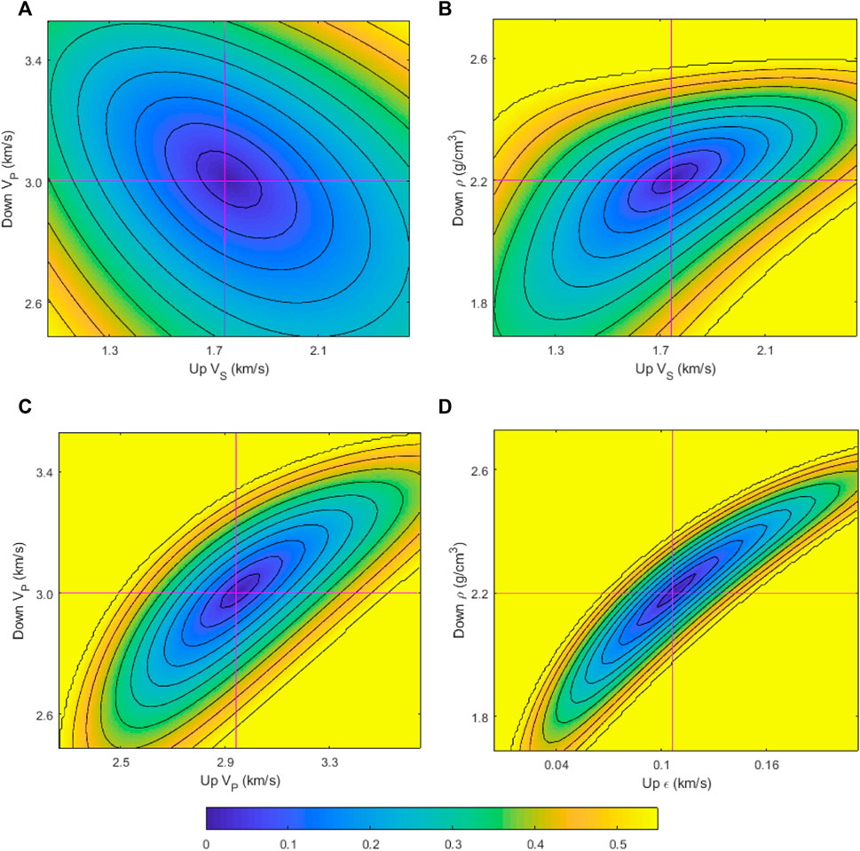
FIGURE 2. Residual function maps. The adjacent contour increment is 0.08. The intersection of the red line represents the corresponding real value. The colorbar at the bottom indicates the corresponding numerical value of each color.

In addition, the introduction of the specific distribution of the prior information of the parameters by Bayesian theory can effectively reduce the uncertainty and non-uniqueness of the inversion and improve the accuracy of results [29,32]. From the above analysis, the nonlinear inversion algorithm combined with Bayesian theory is stable and accurate and does not have a serious non-uniqueness problem.

Application

Synthetic data test

In order to verify the correctness and accuracy of the derivation method in a simple manner, we compared the inversion result with the commonly used VTI media approximation equation [9] and the exact reflection coefficient equation. The reflection coefficient model contains both positive and negative reflection coefficients with thin and thick layers, which is relatively comprehensive. The seismic gather is synthesized by the exact reflection coefficient equation (Figure 3). In the two inversion methods, the 30 Hz ricker wavelet is used.

FIGURE 3

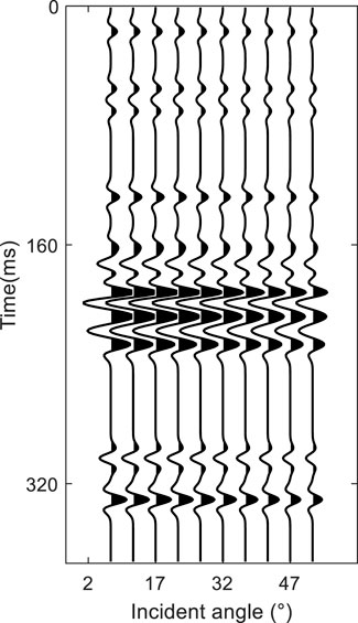
FIGURE 3. Synthetic pre-stack angle gathers. The incident angle is 7°, 12°, 17°, …, 47°.

As shown in Figure 4A, the inversion results based on the exact reflection coefficient equation are very accurate. The inversion results based on the linear reflection coefficient equation are acceptable in trend but lack detail (Figure 4B).

FIGURE 4

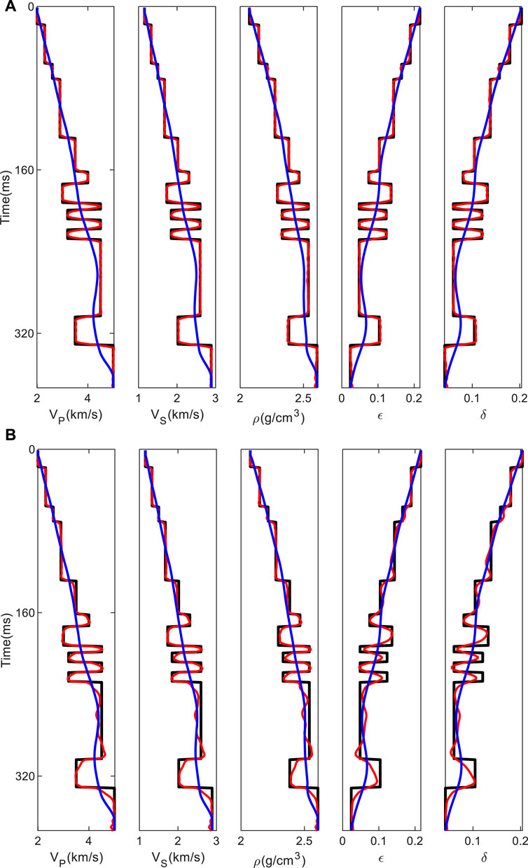
FIGURE 4. Inversion results. The black line indicates the true data, the red line indicates the inversion result, and the blue line indicates the initial data. (A) Accurate nonlinearity inversion; (B) approximate linear inversion.

For testing the feasibility and stability of the inversion algorithm, we apply it to the data that are based on real well logging data. The synthetic pre-stack angle gather is forwarded by the exact VTI reflection coefficient equation. A Ricker wavelet with a dominant frequency of 30 Hz is used in the forwarding process. To test the noise immunity of the inversion algorithm, random noise with a signal-to-noise ratio (SNR) of 2 is added to the seismic gather, as shown in Figure 5.

FIGURE 5

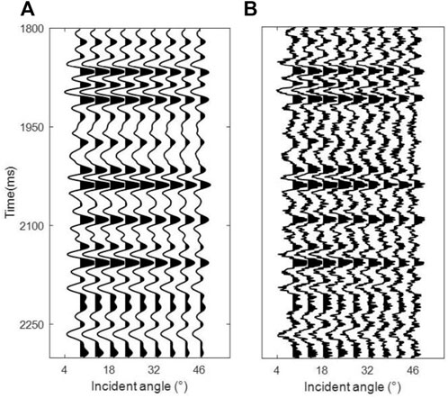
FIGURE 5. Synthetic pre-stack angle gathers: (A) original noiseless data; (B) added random noise SNR = 2. Each angle is 6°, 11°, 16°, …, 46°.

Based on the noiseless seismic data, the Cauchy constrained inversion is implemented; based on noisy seismic data, unconstrained inversion and Cauchy constrained inversion are implemented. From the inversion results (Figure 6), the accuracy of the inversion results based on the exact reflection coefficient equation is quite high in noiseless conditions. In the presence of noise, the inversion algorithm can still predict results reasonably well and the accuracy of the results with the Cauchy constraint is higher. In addition, from the inversion results, the reflection coefficient is less sensitive to the anisotropic parameters and the accuracy of those parameters is slightly lower.

FIGURE 6

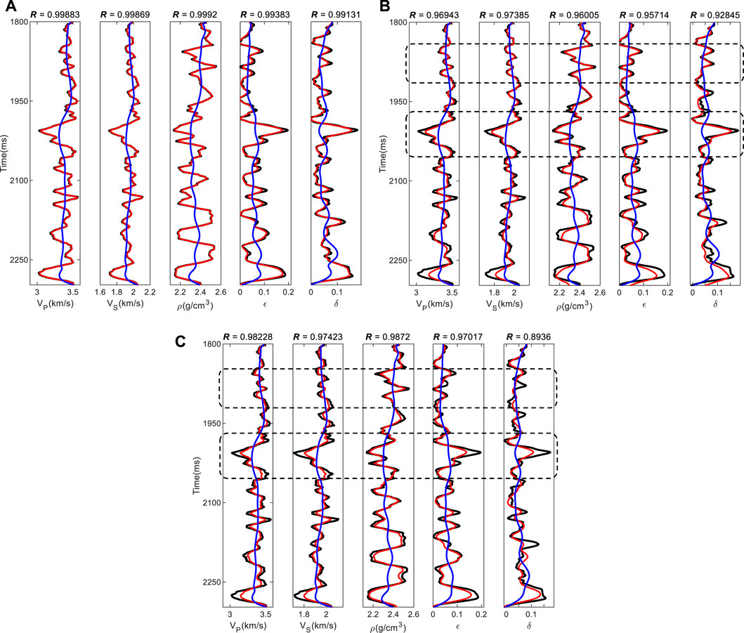
FIGURE 6. Inversion results. (A) Cauchy constraint inversion in noiseless trace gather; (B) Cauchy constraint inversion in SNR = 2 trace gather; (C) Nonconstraint inversion in SNR = 2 trace gather. The black line indicates the true data, the red line indicates the inversion result, and the blue line indicates the initial data. The accuracy of (A) is the highest, the accuracy of (B) is acceptable, and the accuracy of (C) is poor. (A) Shows the feasibility of the inversion algorithm. By comparing (B) and (C) (particularly in the vicinity of black dashed boxes), it can be seen that using the constrained inversion method to process noisy data can increase the accuracy and stability of results.

In conclusion, the proposed inversion method for VTI media can stably and reasonably obtain the elastic parameter information of the formation from the pre-stack seismic data.

Applied to actual work area

We applied the method to Work Area B. This area is located in the middle of the depression, and years of exploration results show that the stratigraphy mainly presents VTI anisotropy. The main lithology is shale, mudstone, and minor sandstone. The main cause of VTI anisotropy is formation pressure. Because the formation is soft and plastic, fractures are not developed and the structure is relatively simple. Figure 7 shows the 200-traces seismic profile with a log. The seismic data was processed by spherical spreading compensation, absorption attenuation compensation, surface-consistent amplitude correction, surface consistent deconvolution, noise suppression, NMO, and pre-stack time migration, among others. Figure 8 is the extracted wavelets of different incident angles. The incidence angles of the seismic gather set are 6°, 15°, 24°, 33°, and 42°. In addition, for feasible inversion using Cauchy constraint in this work area, we conducted a statistical analysis of the elastic parameters of the inversion using logging data; the results show that the Cauchy constraint is more in line with the actual situation of the work area (Supplementary Appendix SB).

FIGURE 7

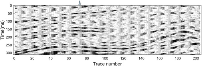
FIGURE 7. Field seismic gather at well location. The well is at trace 73.

FIGURE 8

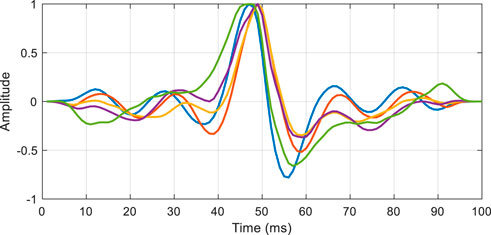
FIGURE 8. Wavelets of different incidence angles. The amplitude is normalized. The corresponding incidence angles are 6° (blue), 15° (green), 24° (orange), 33° (purple), and 42° (yellow). The smaller the angle of incidence, the larger the amplitude of the wavelets, and vice versa.

Figure 9 shows the inversion results, with an accurate spread condition of velocity, density, and anisotropy intensity. The well-bypass inversion result is in good agreement with the coarsened logging data. The inversion results are stable and almost free of noise interference. This shows the accuracy and robustness of the inversion method.

FIGURE 9

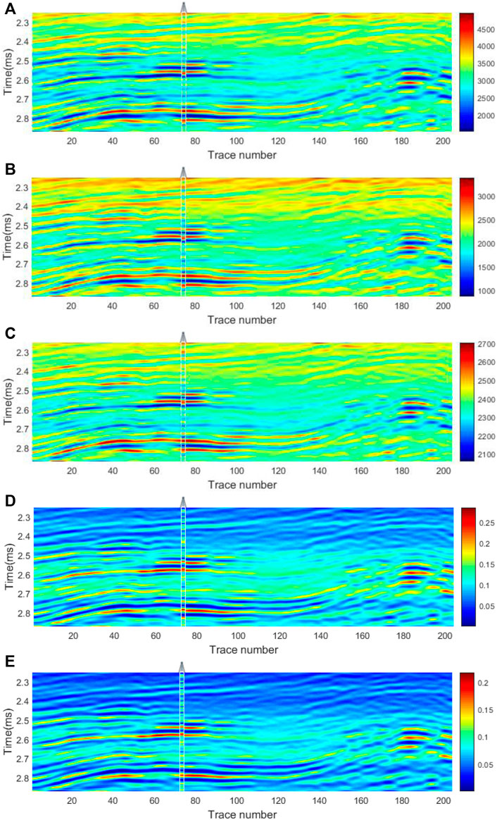
FIGURE 9. Inverted results of exact equation at the well location: (A) P-wave velocity (m/s); (B) S-wave velocity (m/s); (C) density (kg/m³); (D) ε; (E) δ.

In Figure 9, the continuous spreading of each parameter indicates that there is no obvious fracture distribution in this area. This is also revealed in the seismic profile (Figure 7). Figure 9 also shows that the high value areas of velocity and density (Figures 9A–C) are corresponding low values of anisotropic parameters (Figures 9D,E). This indicates that, for subsurface formations, the elastic parameters vary across different rocks. For soft and plastic rocks like shale and mudstone, the velocity and density are low, and these rocks are vulnerable to the effect of formation pressure. This condition easily forms strong VTI anisotropy. For hard and rigid rocks like sandstone, carbonate, and dolomite, the velocity and density are high, and they are less susceptible to the effect of formation pressure. Therefore, the anisotropy is relatively weak. With the description above, the results are a meaningful reference for exploration and construction and provide data for relevant fields.

Conclusion

Humans have a great interest in exploring the Earth’s subsurface. Since direct exploration is impossible, we can use inversion methods. The complexity of geophysical inversion has improved, from the earliest isotropic linear inversion to the later constrained anisotropic nonlinear inversion, in accuracy and stability. It is also closer to the actual subsurface situation.

We derive the generalized linear inversion and iterative reweighted least squares combination algorithm for the exact VTI media reflection coefficient equation. The proposed inversion method can avoid calculation errors introduced from the approximate equations, particularly for far offsets with large angles. The reflection coefficient equation forward curve (Figure 1) and the synthetic data tests also illustrate this point. We managed to protect weak reflections by using the Cauchy distribution as the prior constraint and Bayes’ theorem for application. The statistical analysis of the work area logging data show that it is feasible to use the Cauchy constraint. The objective function is solved with Bayesian theory, which improves the stability and quality of the calculations. The noise immunity is also improved, allowing it to be better applied in actual data. Finally, the method is applied feasibly and effectively in the real work area. The inversion results can provide an accurate understanding of the VTI anisotropy stratigraphic structure and serve further geophysical analysis.

The method can be improved in some respects. Inversion theory with different constraints (Laplace, Markov random field, etc.) [33,34] can be derived to adapt to different situations. The inversion equation of more complex anisotropic media (horizontal transverse isotropic, tilted transverse isotropic, orthorhombic, etc.) can be derived to better adapt to the real underground situation.

Furthermore, the purposed inversion algorithm can also be used for other nonlinear inversion problems. After a simple extension, it can be applied to the joint PP and PS wave inversion. It can also be extended to the pre-stack inversion of multicomponent seismic data (horizontal and vertical components).

Data availability statement

The original contributions presented in the study are included in the article/Supplementary Materials, further inquiries can be directed to the corresponding author.

Author contributions

JL proposed the project and funding the acquisition. FW conducted the equation derivation, simulation, and results processing. WG applied to the actual data. WT wrote and revised the manuscript.

Funding

This work was financially supported by the National Key R&D Program of China (2019YFC0312000), the National Natural Science Foundation of China (41774131 and 41774129), and the research center of CNOOC at Beijing (Grant Number: CCL2021RCPS0196KNN).

Acknowledgments

We would like to thank China University of Petroleum (Beijing) for providing the proprietary information for this study.

Conflict of interest

The authors declare that the research was conducted in the absence of any commercial or financial relationships that could be construed as a potential conflict of interest.

Publisher’s note

All claims expressed in this article are solely those of the authors and do not necessarily represent those of their affiliated organizations, or those of the publisher, the editors and the reviewers. Any product that may be evaluated in this article, or claim that may be made by its manufacturer, is not guaranteed or endorsed by the publisher.

Supplementary material

The Supplementary Material for this article can be found online at: https://www.frontiersin.org/articles/10.3389/fphy.2022.926636/full#supplementary-material

References

1. Crampin S, Chesnokov EM, Hipkin RG. Seismic anisotropy — The state of the art: II. Geophys J Int (1984) 76(1):1–16. doi:10.1111/j.1365-246x.1984.tb05017.x

CrossRef Full Text | Google Scholar

2. Carcione JM, Kosloff D, Behle A. Long-wave anisotropy in stratified media: A numerical test. Geophysics (1991) 56:245–54. doi:10.1190/1.1443037

CrossRef Full Text | Google Scholar

3. Wang Z. Seismic anisotropy in sedimentary rocks, part 2: Laboratory data. Geophysics (2002) 67:1423–40. doi:10.1190/1.1512743

CrossRef Full Text | Google Scholar

4. Henneke EG. Reflection-refraction of a stress wave at a plane boundary between anisotropic media. J Acoust Soc Am (1972) 51:210–7. doi:10.1121/1.1912832

CrossRef Full Text | Google Scholar

5. Graebner M. Plane‐wave reflection and transmission coefficients for a transversely isotropic solid. Geophysics (1992) 57(11):1512–9. doi:10.1190/1.1443219

CrossRef Full Text | Google Scholar

6. Daley PF, Hron F. Reflection and transmission coefficients for transversely isotropic media. Bull Seismological Soc America (1977) 67(3):661–75. doi:10.1785/bssa0670030661

CrossRef Full Text | Google Scholar

7. Rüger A. Reflection coefficients and azimuthal AVO analysis in anisotropic media, Colorado: Colorado School of Mines (1996). dissertation/doctor’s thesis.

8. Thomsen L. Weak anisotropic reflections: In offset-dependent reflectivity-theory and practice of AVO analysis. United States: Society of Exploration Geophysicists (1993) 103–14.

Google Scholar

9. Rüger A. P-wave reflection coefficients for transversely isotropic models with vertical and horizontal axis of symmetry. Geophysics (1997) 62(3):713–22. doi:10.1190/1.1444181

CrossRef Full Text | Google Scholar

10. Jílek P. Converted PS-wave reflection coefficients in weakly anisotropic media. Pure Appl Geophys (2002) 159(7-8):1527–62. doi:10.1007/s00024-002-8696-9

CrossRef Full Text | Google Scholar

11. Shaw RK, Sen MK. Born integral, stationary phase and linearized reflection coefficients in weak anisotropic media. Geophys J Int (2004) 158:225–38. doi:10.1111/j.1365-246x.2004.02283.x

CrossRef Full Text | Google Scholar

12. Plessix RE, Bork J. Quantitative estimate of VTI parameters from AVA responses. Geophys Prospecting (2000) 48:87–108. doi:10.1046/j.1365-2478.2000.00175.x

CrossRef Full Text | Google Scholar

13. Zhang T, Zhang F, Li XY. (2017). Anisotropic inversion for the VTI media based on a three-term AVO equation. 79th Annual International Meeting, Jun 2017, EAGE, Conference & Exhibition.

CrossRef Full Text | Google Scholar

14. Zhang F, Li XY. Generalized approximations of reflection coefficients in orthorhombic media. J Geophys Eng (2013) 10:054004–403. doi:10.1088/1742-2132/10/5/054004

CrossRef Full Text | Google Scholar

15. Zhang F, Li XY (2014). Simultaneous inversion of elastic and anisotropy parameters for a clay-rich shale formation. In, SEG Expanded Abstracts, 84th Annual Conf. of the Soc. of Exploration Geophysics, Aug 2014 569–73.

CrossRef Full Text | Google Scholar

16. Kim KY, Wrolstad KH. Effects of transverse isotropy on P‐wave AVO for gas sands. Geophysics (1993) 58(6):883–8. doi:10.1190/1.1443472

CrossRef Full Text | Google Scholar

17. Amit P, Subhashis M (2013). Accurate estimation of VTI media parameters using multicomponent prestack waveform inversion. 83th Annual International Meeting, Sept 2013, SEG, Expanded Abstracts: 1664–8.

Google Scholar

18. Thomsen L. Weak elastic anisotropy. Geophysics (1986) 51(10):1954–66. doi:10.1190/1.1442051

CrossRef Full Text | Google Scholar

19. Schoenberg M, Protázio J. Zoeppritz" rationalized and generalized to anisotropy. J Seismic Exploration (1992) 1:125–44.

Google Scholar

20. Zoeppritz K. On reflection and propagation of seismic waves. Gottinger Nachrichten (1919) 1:66–84.

Google Scholar

21. Aki K, Richards PG. Quantitative seismology. Theory and methods. United States: W. H. Freeman (1980).

Google Scholar

22. Tarantola A. Inverse problem theory and methods for model parameter estimation. Philadelphia: SIAM (2005).

Google Scholar

23. Downton JE. Seismic parameter estimation from AVO inversion, Calgary: University of Calgary (2005). dissertation/doctor’s thesis.

24. Alemie W, Sacchi MD. High-resolution three-term AVO inversion by means of a Trivariate Cauchy probability distribution. Geophysics (2011) 76(3):R43–R55. doi:10.1190/1.3554627

CrossRef Full Text | Google Scholar

25. Wang YM, Wang XP, Shen SQ (2009). Pre‐stack multi‐angle three‐parameter synchronous inversion method. SEG Global Meeting Abstracts, Jun 2011 258–258.

CrossRef Full Text | Google Scholar

26. Chen TS, Wei XC (2012). Zeoppritz-based joint AVO inversion of PP and PS waves in Ray parameter domain. 82th Annual International Meeting, Oct 2012, SEG, Expanded Abstracts: 1–5.

CrossRef Full Text | Google Scholar

27. Lu J, Yang Z, Wang Y, Shi Y. Joint PP and PS AVA seismic inversion using exact Zoeppritz equations. Geophysics (2015) 80(5):R239–50. doi:10.1190/geo2014-0490.1

CrossRef Full Text | Google Scholar

28. Zhi LX, Chen SQ, Li XY. Amplitude variation with angle inversion using the exact Zoeppritz equations -Theory and methodology. Geophysics (2016) 81(2):N1–N15. doi:10.1190/geo2014-0582.1

CrossRef Full Text | Google Scholar

29. Macdonald C, Davis PM, Jackson DD. Inversion of reflection traveltimes and amplitudes. Geophysics (1987) 52(5):606–17. doi:10.1190/1.1442330

CrossRef Full Text | Google Scholar

30. Larsen JA. AVO inversion by simultaneous P-P and P-S inversion. Calgary: University of Calgary (1999).

Google Scholar

31. Castagna J, Backus M. Offset-dependent reflectivity—Theory and practice of AVO analysis. United States: Society of Exploration Geophysicists (1993). p. 287–302.

Google Scholar

32. Downton JE, Lines LR (2001). Constrained three parameter AVO inversion and uncertainty analysis. 71th Annual International Meeting, Sept 2001, SEG, Expanded Abstracts 251–4.

CrossRef Full Text | Google Scholar

33. Wang P, Cui Y, Wang S, Zhang P, Zhu G, Meng J. (2022). Probabilistic prediction of elastic parameters constrained by sparse lithology prior. 83rd EAGE Annual Conference & Exhibition Conference paper, Jan 2022, 1–5.

CrossRef Full Text | Google Scholar

34. Wang P, Cui Y, Du XZ. Improved prior construction for probabilistic seismic prediction. IEEE Geosci Remote Sens Lett (2022) 19:1–5. doi:10.1109/lgrs.2022.3175966

CrossRef Full Text | Google Scholar

37. Keith C. M., Crampin S. Seismic body waves in anisotropic media: Reflection and refraction at a plane interface. Geophys. J. Roy. Astr. Soc. (1977) 49:181–208.

CrossRef Full Text | Google Scholar