- School of Management, University of Science and Technology of China, Hefei, China
This article applies several distinct methods including the systemic linkage method and network analysis to address intranational systemic risk interdependencies. Specifically, we initially quantify dynamic systemic linkages among US and Chinese systemically important financial institutions through time-varying adjacency matrices related to an extreme value theory (EVT) approach and then visualize them using network analysis. Numerical and graphical results show that intranational systemic linkages are obviously enhancive under extreme scenarios such as large negative shocks in the financial system. In addition, we apply a tail event-driven network quantile regression (TENQR) model to address the interdependence and dynamics of the entire network. The estimation results show that the network factors respond more strongly when the market suffers extreme stress.
1 Introduction
The global financial crisis of 2007–2008 accented the great extent to which the failure of an interconnected and complex financial institution can jeopardize the stability of the entire financial system. In view of this concern, new macroprudential financial regulations put greater emphasis on systemic risk, that is, the interconnectedness of risk among institutions, especially those that are “too big to fail”.
Forbes and Rigobon [1] and Casarin et al. [2] interpret contagion as a significant increase in cross-market correlation during a period of financial turmoil, whereas any continued high market correlation is defined as interdependence. According to the Financial Stability Board, systemically important financial institutions (SIFIs) are financial institutions whose disorderly failure, because of their size, complexity and systemic interconnectedness, would cause significant disruption to the wider financial system and economic activity. In this context, the analysis of risk interdependence among SIFIs plays an important role in quantifying and assessing financial systemic risk.
Recent decades have seen considerable research into the mechanisms behind systemic risk (e.g., [3–6]). De Bandt and Hartmann [7] divide a systemic event into two key component types: shocks and propagation mechanisms. In a strict sense, idiosyncratic shocks initially affect only the stability of a single financial institution or only the price of a single asset, while systematic shocks propagate from one financial institution or market to others and may even affect the entire economy. Likewise [8]) demonstrate that systemic risk builds up in the background during the expansion phase of imbalances or bubbles and materializes only when the crisis erupts.
Systemic risk measures have become particularly crucial since the implementation of the Basel II bank regulations and proliferated following the global financial crisis. The purpose of risk measures is to reduce vast volumes of data to a meaningful single statistic that summarizes risk. Bisias et al. [9] provide a survey of over 30 quantitative systemic risk measures in the economics and finance literature. One of the most common measures of risk, which is set as the official measure of market risk under Basel II, is value-at-risk (VaR). VaR is simply defined as the worst expected loss of a position over a target horizon within a given confidence interval. Although not a coherent risk measure, VaR is immensely popular. Other widespread risk measures, including conditional value-at-risk (CVaR) [10], marginal expected shortfall (MES) [6, 11] and a systemic risk measure called SRISK [12], have better formal properties than the standard VaR. These approaches, which rely on market data to produce global measures, can be calculated in a timely manner to better detect sudden fluctuations in the financial system. Benoit et al. [13] classify this kind of measure as representative of the global approach, which aims to derive global measures of systemic risk. Our proposed risk measure in this paper is also categorized within the global approach [14].
Our study is related to the work of Van Oordt and Zhou [14]. Using extreme value theory (EVT), they decompose banks’ systemic risk into two dimensions: the risk of individual institutions (bank tail risk) and the link of the bank to the system in financial distress (systemic linkage). Their proposed systemic risk measure and its decomposition help to establish a connection between studies applying tail dependence as a proxy of systemic risk [15–19] and those applying other global measures such as CoVaR, MES and SRISK. To illustrate the interconnectedness among SIFIs from a system-wide perspective, we further add a topological network methodology to our framework as a necessary supplement. Network analysis is recognized as a powerful methodological tool for modeling interactions between financial institutions and assessing the resilience of financial systems to systemic risk [20–23]. Related network techniques have been used, among other purposes, to describe the global architecture of cross-border financial flows [24], to analyze financial contagion [25, 26] or tail risk spillover [27, 28], and to evaluate credit risk [29].
In this paper, we adopt a risk measure combining the systemic linkage method and network analysis to address intranational systemic risk interdependencies. SIFIs, by definition, occupy crucial positions in the financial system due to their large scale, complex structures, wide range of businesses and strong correlations with other financial institutions in the system. Using daily stock returns on American and Chinese SIFIs, we describe the topology of the network using different metrics of interconnectedness and assess its dynamics. First, we adopt the systemic linkage component of the systemic risk decomposition proposed by Van Oordt and Zhou [14] to measure the strength of the link between individual institutions and the system in financial distress. The difference between our study and theirs lies in the calculation of the component. We directly utilize the sliding window algorithm to calculate time-varying systemic linkages, whereas they adopt regression models to calculate the systemic linkages. Since the systemic linkage component performs only weakly in quantifying systemic risk from a system-wide perspective, we next apply a network analysis technique called the tail event-driven network quantile regression (TENQR) model [30]. We use estimated systemic linkages to construct time-varying adjacency matrices to portray the dynamic networks of SIFIs.
Our major contribution has several aspects. First, this paper applies the systemic linkages to network analysis and measure how closely linked two financial institutions are in periods of financial distress. The combination of systemic linkages and conventional network topology enriched the current literature on network analysis. Using this risk profile, we can construct a more comprehensive and precise network, as displayed in the empirical results. Second, we add the dynamics into the systemic linkages by means of a sliding window, which captures the interplay among SIFIs in different stages. In addition, we take both the US and the Chinese stock markets into account and divide them into three separate periods according to their own features.
The remainder of this paper is structured as follows. In Section 2, we provide the details of our methodology, including the systemic risk decomposition, the construction of the adjacency matrix, and the TENQR network model, where we focus on the dynamic interplay of the networks. Section 3 introduces the data. Section 4 presents the empirical results. Conclusions are presented in Section 5.
2 Systemic Risk Modeling Analysis
In this section, we lay out the background and preliminaries of our systemic risk analysis, which can be divided into three primary parts: the decomposition of systemic risk, the construction of the adjacency matrix, and the network dynamics based on a TENQR model.
2.1 Systemic Risk Measure
The emergence of systemic risk is receiving increasing attention among regulators, with a particular focus on financial interconnectedness. One natural approach to measuring interconnectedness is through the return sensitivity to key risk factors, the coefficient of a linear relationship between one financial institution and another [31]. Consider a linear tail model between the equity returns of financial institution i and financial institution j upon extremely adverse shocks in the financial system:
where Ri and Rj denote the stock returns of financial institution i and financial institution j,
There are various ways to estimate
where VaRi(p) and VaRj(p) are the VaRs of Ri and Rj with a probability level p and τi(p) is defined as
which can be regarded as the tail dependence measure between Ri and Rj intuitively with 0 ≤ τi ≤ 1. As in conventional extreme value analysis, with n independent and identically distributed (i.i.d.) observations of (Ri, Rj), we consider only the lowest k observations in the tail region, where k is a sequence depending on n such that k≔k(n) → +∞ and k/n → 0 as n → +∞. Hence, according to Eq. 2, we can obtain the estimator of
where
where Ri,(k+1) and Rj,(k+1) are the (k+1)th lowest-order statistics of Ri and Rj and
2.2 Decomposition of Systemic Risk
We further address the problem of how individual financial institutions influence each other. Drawing on the seminal work of Van Oordt and Zhou [14], this part decomposes the systemic risk of a financial institution into the tail risk and the systemic linkage. Van Oordt and Zhou [14] consider the logarithmic transformation of
which divides the systemic risk measure
2.3 Adjacency Matrix
To explore the relationship or the interconnectedness among SIFIs from a system-wide perspective, we further carry out a tailored network analysis based on graph theory. Graph theory is the study of graphs, specifically the relationship among edges and vertices, which are basic graph elements. This theory offers a practical tool to analyze and visualize the complexities of interactions. In our study, each vertex represents a specific SIFI, and each edge indicates the dependence or channel between two financial institutions. The relationship between vertices/nodes and edges is described by an adjacency matrix A with elements aij, which determine the weights of edges between i and j. With n vertices, A is an (n × n) square matrix. Thus, a basic undirected graph is defined as follows:
The equation above is the simplest case of a network structure in which all edges share the same weight with one (zero) used to represent a link (isolation). However, the network between SIFIs is time varying and directional since there is a risk contributor and a risk receiver in a relationship. Hence, to capture the dynamic interplay between financial institutions upon the occurrence of tail events in time, we take the systemic linkage mentioned in Section 2.2 as a risk profile. At each time point t, an n-dimensional adjacency matrix At composed of elements aij,t = SLij,t can be defined as:
Each institution i is characterized by a vector
2.4 Tail Event-Driven Network Quantile Regression
To determine the dynamic adjacency relation among SIFIs, in this section, we introduce a parsimonious model, the tail event-driven network quantile regression model. Given the aforementioned definition of SLij, we obtain pairwise systemic linkages between two arbitrary financial institutions. In practice, it is not advisable to take all systemic linkages into consideration. Based on a breakpoint technique, we identify large systemic linkages whose value must exceed an approximate threshold.
2.4.1 Breakpoint Approach
Denote
Here, we have ϕk ∈ [0, 1] since SLk ∈ [ − 1, 1]. Following previous work by Chen et al. [30], we denote the spacings as Δk = ϕk − ϕk−1. To split the sequence of spacings into subsets using a cluster approach, we denote θ as the fraction of spacings that separates high systemic linkages, which is estimated by
where
where ν(i, j) is the mapping that assigns to each pair (i, j) of SIFIs the index of the ordered systemic linkages.
2.4.2 Tail Event-Driven Network Quantile Regression Model
We further pay attention to the tail dynamics. Initially, it is of great interest to quantify the reaction of an individual SIFI at a specific time point to the connection at the previous time point. In addition, the yield of an individual SIFI may show an asymmetrical response to network factors. In other words, the node may respond more strongly under extremely adverse situations but more mildly under advanced conditions.
To avoid the curse of dimensionality, Chen et al. [30] propose a parsimonious model called the tail event-driven network quantile regression (TENQR) model to address tail sensitivities, asymmetric impacts, intertemporal effects, regional reactions and impulse responses to network shocks. One advantage of this applied quantile regression, relative to an ordinary least squares regression, is that TENQR estimates are more robust against outliers in the response measurements. In the context of our own TENQR model, we concentrate on tail events such as high-level quantiles. Specifically, we use the systemic linkage as a risk profile to calculate network factors and omit regional reactions and add universally used explanatory factors such as autoregressive components, market-wide covariates and company-specific variables. The time variations are reflected via returns Ri,t, and the TENQR model of Ri,t is defined as follows:
where t = 1, … , T and i = 1, … , n. γi,t represents the residuals. Wl,t represents the market-wide covariates at a given time point t. The CBOE Volatility Index (VIX), also referred to as the “fear gauge,” is a popular measure of volatility expectations for the US stock market. A higher VIX means that market participants expect more intense market volatility. In addition, we consider the TED rate, which refers to the difference between the Treasury bill yield and the London Interbank Offered Rate. The rate is fairly small in normal circumstances, but when market-wide credit default risk is increasing, the TED spread becomes higher. Thus, the TED rate is an ideal index to assess market-wide credit risk. In our model, we choose the VIX as a proxy for perceived market sentiment and the TED rate for perceived credit risk. mi(Rj,t−1) is a function of neighboring nodes that have connectedness with node i. The coefficient αf(τ) correspondingly measures the impact of the network factors and is merely dependent on τ. The construction of the mi-function is based on adjacency matrices with elements according to Eq. 10, and the network factors are defined as:
in which the network factors fi are regarded as weighted average impacts from nodes that are connected with the ith node.
3 Data
This paper uses equity returns to calculate the systemic risk measure and its systemic linkage subcomponent. We take two global stock markets, the US stock market and the Chinese stock market, as empirical examples. The dataset used in this paper is selected with reference to Brownlees and Engle [36] and Banulescu and Dumitrescu [37], with a few changes in consideration of their market capitalization, liabilities, trading volumes and reputations.
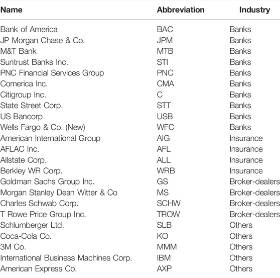
Since the US stock market is the maturest and largest market, with rigorous and transparent management, we select it as the setting from which we extract our first dataset, which covers the period between January 2006 and December 2019. The development of and changes in the US stock market played out within a momentous global political and economic historical context. Thus, it is appropriate to take this market into account. To ensure the reliability of the research, the data are processed as follows: 1) we delete the stocks of financial institutions with data missing for more than 90 days; and 2) we use the closing price of the previous trading day to replace small amounts of missing data. Finally, we obtain 23 listed financial institutions that can be divided into four sectors: 1–10 are banks (e.g., Bank of America, JP Morgan), 11–14 are insurance companies (e.g., American International Group), 15–18 are broker-dealers (e.g., Morgan Stanley), and 19–23 are others (e.g., 3M). The financial data come from the Wind Financial database, and detailed information, including names, abbreviations and sectors, is listed in Table 1. To better study the risk correlations among SIFIs under different market conditions around the 2007–08 global financial crisis, we examine daily data covering three subperiods: 1) stage 1: the prefinancial crisis period, ranging from January 2006 to July 2007; 2) stage 2: the period during the financial crisis itself, from August 2007 to June 2009; and 3) stage 3: the postfinancial crisis period, ranging from July 2009 to December 2019.
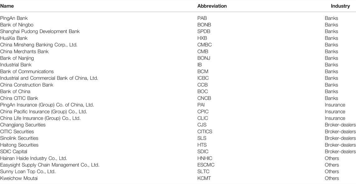
For emerging markets, we select the Chinese stock market, the second largest stock market worldwide, as our second testing ground. Unlike mature markets, emerging markets are characterized by relatively pooled enforcement of financial regulations. We are interested in risk transfers among Chinese SIFIs. Following Huang and Wang [38], our selection mechanism is based on the guidelines for the Industry Classification of Listed Companies issued by China Securities Regulatory Commission, and we deal with the raw data in the similar way as for the US SIFIs. In the following analysis of the Chinese stock market, we focus mainly on systemic risk during 2014–16, when the Chinese stock market experienced evident fluctuations. As the focus of this article is not to compare the systemic networks of the Chinese market with those of the US market, we choose different periods that have the most impact on each market. Eventually, we choose 25 listed Chinese SIFIs, including 13 banks (e.g., China Merchants Bank, Bank of China), 3 insurance companies (e.g., PingAn Insurance), 5 broker-dealers (e.g., Changjiang Securities, CITIC Securities) and 4 others (e.g., Haide Industry). We collect their daily closing prices from January 2013 to December 2019. Likewise, we consider three separate periods: 1) stage 1: the precrash period, ranging from January 2013 to June 2014; 2) stage 2: the period during the Chinese stock crash from July 2014 to January 2016; and 3) stage 3: the postcrash crisis period, ranging from February 2016 to December 2019. Table 2 presents the names, abbreviations and sectors of the listed Chinese SIFIs.
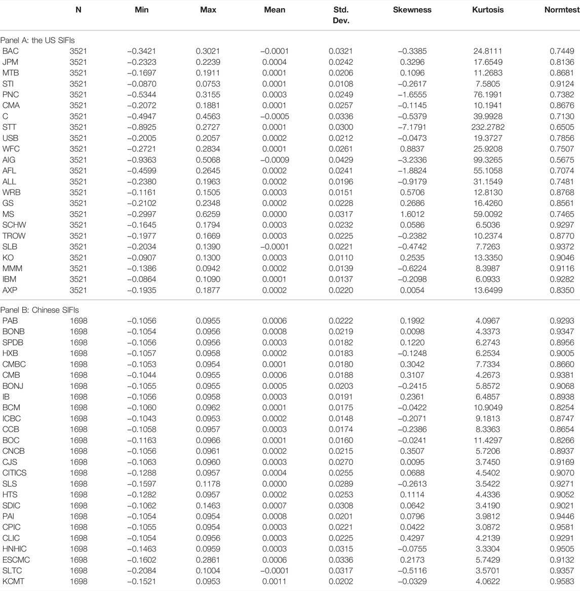
Our analysis centralizes the daily log returns of each SIFI. Table 3 presents the descriptive statistics for returns of 23 US SIFIs and 25 Chinese SIFIs during the full sample period. First, we note that all the means of returns are positive, except for BAC, C, AIG and SLB for Panel A and IB for Panel B. Second, all return series exhibit non-zero skewness and show high kurtosis (excess 3), which is reflected in the rejection of the null hypothesis of normality (the last column of Table 3 presents the statistic of a Shapiro-Wilk test of normality).
4 Empirical Application
In this section, we apply the technique previously presented and propose an empirical application of our risk methods to identify and measure the systemic risk of listed SIFIs. Using daily logarithmic returns and the sliding window algorithm, we estimate the systemic linkages of each stock market. Similar to the specification in Longin and Solnik [39] and Van Oordt and Zhou [14], we set the window width = 20 representing an estimation window of 2 years of daily returns and k/n ≈ 0.04 to obtain the time-varying systemic linkages SLij,t as described in Section 2.2. Then, we construct dynamic adjacency matrices At and the networks of SIFIs and refine them by applying the breakpoint approach mentioned in Section 2.4.1. Finally, the TENQR model is applied to address the tail sensitivities and dynamics.
4.1 Dynamic Systemic Linkage Table
To better visualize the changes in data over time, we further use heat maps to display the variations in systemic linkages in different stages. First, we compute the mean value of systemic linkages to generate a systemic linkage matrix table for each stage. Second, we calculate the difference based on the three systemic linkage tables to obtain the two target systemic linkage variation tables—for stage 1 to stage 2 and for stage 2 to stage 3. Then, we apply a heat map since the colors are easier to distinguish and make sense of than raw numbers. The warmer the color, the larger the value.
Figure 1 displays the systemic linkage variations of the US SIFIs. Obviously, the influence of different SIFIs in different periods varies greatly. We notice that in Figure 1A, corresponding to the case of the systemic linkage variations from stage 1 to stage 2, the values are significantly positive. Specifically, approximately 52.36% of the values (or 68.62%) are over 0.1 (or 0.05), and only 1.70% (or 5.86%) are below −0.1 (or −0.05). It is obvious that several pairs of systemic linkage variation excess 0.3, e.g., JPM and USB. As a whole, there are more systemic spillovers between banking sectors, emitting more risk to the system than other sectors. This finding is in line with that of Härdle et al. [40] who suggest that broker-dealers and others fluctuate very much in the whole period, but they send out less risk compared with banks. They also find that JPM and USB are ranked in the top 10 largest systemic risk emitters list. Besides, it is noted that in others sector, the systemic linkage variation between AXP and MMM is up to 0.34, reflecting they are highly linked in global financial crisis. Other studies including Diebold and Yılmaz [22] and Härdle et al. [40] have indicated that AXP is a large systemic risk contributor.
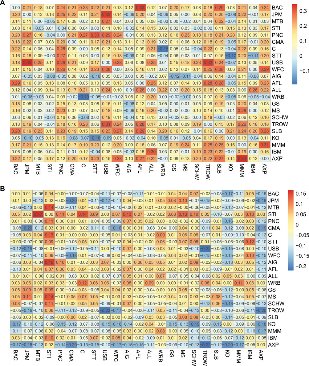
FIGURE 1. Systemic linkage variation table for the US SIFIs. (A) Systemic linkage variation table from stage 1 to stage 2. (B) Systemic linkage variation table from stage 2 to stage 3.
In contrast in Figure 1B, the values decrease since only 3.40% (or 14.37%) are above 0.1 (or 0.05) and 19.10% (or 38.75%) are below −0.1 (or −0.05). This phenomenon can also be observed from the color change. The colors in 1) are warmer than those in 2) overall. This suggests that from stage 1 to stage 2, the systemic risk correlation becomes obviously higher, and from stage 2 to stage 3, the correlation becomes weaker on average. However, some exceptions still exist. For instance in Figure 1B, the systemic linkage variation between MTB and STI is 0.17, perhaps due to the intra-industry information transfer. The correlations among the SIFIs in stage 2, or during the financial crisis, tend to increase, and the systemic risk contagion effect is significant.
Similarly, the systemic linkage variations of the Chinese SIFIs are shown in Figure 2. The difference in the color of the two heat maps is apparent at first glance. Most of the values in Figure 2B are in cool colors. Statistically, for Figure 2A, 25.60% (or 38.88%) of the values exceed 0.1 (or 0.05), and 8.16% (or 22.08%) are lower than -0.1 (or -0.05). We note that the high values of systemic linkage variation is linked with IB, ICBC and KCMT, which is a reflection of the high capability to emit and receive systemic risk. Wang et al. [41] points out that IB is considered as “interbank king” in China’s financial system. At the end of 2016, the interbank liabilities of IB reached over 1.72 trillion yuan, accounting for one third of their total liabilities. As a result, regulators should pay more attention to IB with significant exposure to shadow banks.
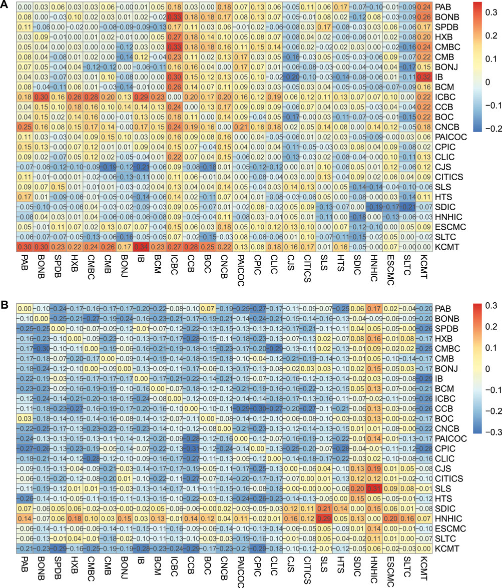
FIGURE 2. Systemic linkage variation table for the Chinese SIFIs. (A) Systemic linkage variation table from stage 1 to stage 2. (B) Systemic linkage variation table from stage 2 to stage 3.
Figure 2B, however, shows that only 3.84% (or 9.12%) of the values exceed 0.1 (or 0.05) and more than half (57.12%) are below −0.1, while up to 72.48% are less than −0.05. These statistics are consistent with what the heat maps show that from stages 2 to 3, the values of systemic linkages visually become smaller, indicating that after the financial crisis, the correlations among the Chinese SIFIs become significantly weaker overall except an outlier between SLS and HNHIC. In the work of Wang et al. [41], they reveal that both CJS and SLS receive the most tail risk. In addition, they mention that securities triggered the recent bull market in 2016, which is not found in our paper. These findings above confirm the similarity with the results for the US SIFIs that in periods of financial distress, SIFIs are more linked than they are before or after the distress.
4.2 Network Visualization
In this section, we apply the aforementioned breakpoint approach to simplify the original systemic linkage tables and obtain refined systemic linkage tables. Figures 3, 4 visually portray the systemic risk dependence networks of the US SIFIs and Chinese SIFIs over the three separate stages. We select one time point for each stage in our examples. Arrows denote the direction of the impact between paired SIFIs.

FIGURE 3. Systemic risk dependence networks of the US SIFIs across the three stages. (A) Stage 1 (17 October 2006) (B) Stage 2 (20 December 2007) (C) Stage 3 (28 January 2013).

FIGURE 4. Systemic risk dependence networks of the Chinese SIFIs across the three stages. (A) Stage 1 (7 November 2013) (B) Stage 2 (24 April 2015) (C) Stage 3 (9 December 2016).
According to the network figures, we observe that intuitively, the grave crises such as the 2007–08 global financial crisis and the 2014–16 stock crash saw an increase in the systemic linkages among the SIFIs, which reflects higher risk levels of spillover effects. The network is relatively sparse during the tranquil period, but becomes dense when the financial system encounters extreme conditions, especially when severe shocks occur. In contrast, under mild conditions (stage 1 and stage 3), the network of the systemic linkages is weaker, which shows a weak system-wide connectedness. This result is consistent with Härdle et al. [40] and Fang et al. [42], supporting that losses can spread quickly among financial institutions and threaten the entire financial system during a crisis. Strong linkages tend to occur among SIFIs that belong to the same or a similar industry. The graphical visualization of pairwise risk spillovers is consistent with the results in later tables (Tables 4, 5). This helps to explain the “too-connected-to-fail” situation and to identify potential economic crises.
4.3 Network Centrality
Centrality is one of the most studied concepts in social network analysis [43]. It is a vital index since it indicates which node occupies a critical position. Existing measures include degree centrality, closeness, betweenness, eigenvector centrality, information centrality, flow betweenness, the rush index, etc. In the following network analysis, we apply degree centrality as proposed by Freeman et al. [44], which is measured by the total number of direct links with other nodes. In other words, the measure is the sum of each row in the adjacency matrix representing the network. The degree is the number of directly connected edges, and hence, we evaluate direct connections. For directed graphs, we have to distinguish the in-degree and out-degree [45, 46], which measure the total number of risk transmitters (incoming) and risk recipients (outgoing), respectively. We let the element aij = 1 if there is an edge from institution j to i. Denote the in-degree and out-degree values as degreei,in and degreei,out, respectively, and we have
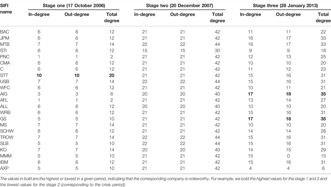
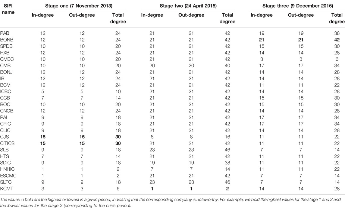
Tables 4, 5 summarize the in-degree, out-degree and total degree of the US and Chinese SIFIs over the three stages in accordance with the definitions in Eqs 13–15.
In conducting the degree analysis for the US network in stage 1 (Table 4), we note that most values of the total degree are between 10 and 14, and STT in the banking industry displays the highest level for all degrees. STT is chosen as the central SIFI and identified as a cluster. This means that STT affects the largest number of other SIFIs and is more sensitive to shock spillovers. Founded in 1792, STT is one of the world’s largest servicers and managers of institutional assets. The corporation, through its subsidiary State Street Bank, provides a range of financial products and services to institutional investors worldwide. It occupies a certain position and wields some influence in the industry, even in the entire market. On the other hand, we observe that the least significantly affected are PNC and AFL, whose total degree value is only 2. However, in stage 2, when the severe financial crisis occurs, the numerical values become larger, and more SIFIs are connected regardless of industry. Almost all values of the total degree are no less than 40. This finding is consistent with the common conclusion that systemic risk rises during a market shock. No SIFIs or industry were immune from the global financial crisis. In stage 3, where the economy returns to a mild situation, the risk association among SIFIs weakens. Large-scale insurers, such as AIG, and broker-dealers, such as GS, are central SIFIs.
Similar results are observed in Table 5. It is clear that in stage 1, CJS and CITICS are the most influential SIFIs in the system, as they affect the highest number of SIFIs (both the in-degree and out-degree are the highest). The finding is consistent with Hautsch et al. [47] and Fang et al. [42] who suggest that these firms like CJS, BONB and CITIC amplify tail risk spillovers. For stage 2, the values of the average total degree are much larger than those in other stages. We obtain the same finding in the case of the US that more SIFIs are closely connected, during the Chinese stock crash. This makes sense since in market turmoil, the linkages between SIFIs would be exacerbated. In comparison to the results reported in the literature, we note that Wang et al. [41] have mentioned that ICBC, CCB and BOC are the top three systemic risk receivers and emitters, especially during the period from mid-2014 to mid-2016 (covering the bullish period and the market turbulence). Additionally, we observe KCMT in the other industries category is an exception. Due to its high liquidity and stable performance, KCMT has become the preferred option pursued by institutional investors. When the system encounters a crash, KCMT is relatively less exposed to the risk of collapse in the entire system. After the crash, we observe that BONB in the banking industry is the most central SIFI since it has the highest degree value. This result is also consistent with that of Fang et al. [42].
4.4 Results From the Tail Event-Driven Network Quantile Regression Model
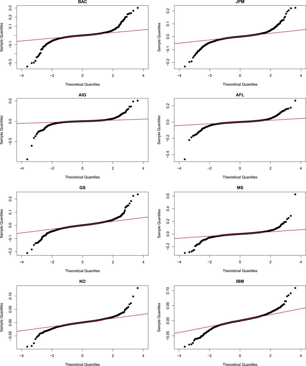
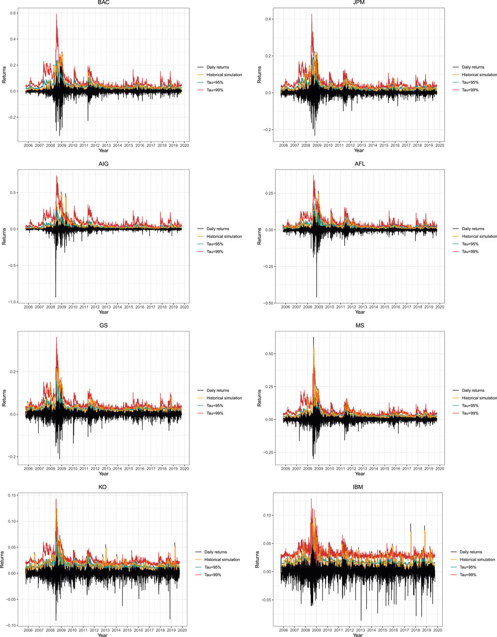
In this section, we apply the TENQR model defined in Section 2.4.2 to the daily return data for the 23 US SIFIs to address tail sensitivity. Due to space limitations, we choose two SIFIs for each industry listed in Table 1. Figure 5 presents the normal QQ plots of the returns of BAC, JPM, AIG, AFL, GS, MS, KO and IBM. It is no surprise that all the returns exhibit heavy tails. We evaluate the impacts of network factors fi using systemic linkages. Specifically, we estimate the TENQR model of Ri,t in the case of τ = 0.95 and τ = 0.99. For comparison, we also take the conventional historical simulation method into consideration when τ = 0.99. We pay more attention to the tails. Figure 6 shows the conditional quantile regressions of BAC, JPM, AIG, AFL, GS, MS, KO and IBM in stage 2, when the severe financial crisis occurs.
From Figure 6, we note that the TENQR model performs better than the historical simulation method in the case of τ = 0.99 and τ = 0.95. It is known that when the financial system is shaky, the VaR calculated by the historical simulation method tends to underestimate systemic risk, whereas our TENQR model takes the tail effect into greater account. Consequently, the TENQR model based on systemic linkages may better reflect the magnitude of systemic risk than the conventional VaR model.
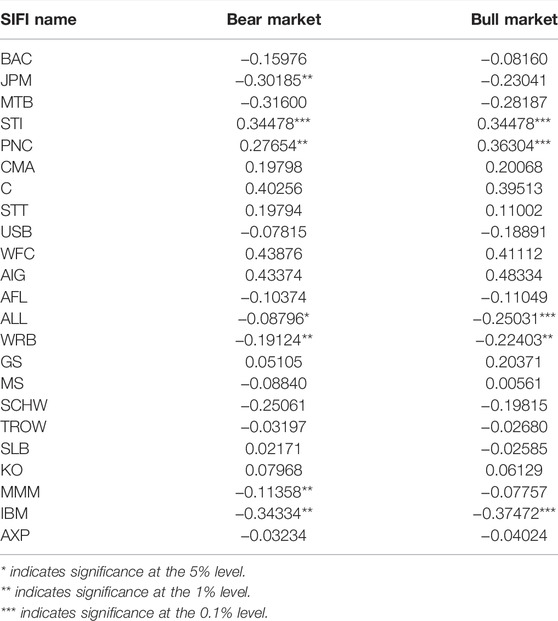
To assess the impacts of network factors under bull and bear markets, we calculate the dynamic fi at each time point t. Empirically, we set a fixed 20-day backward horizon. Table 6 displays the network influences of the 23 US SIFIs in case of τ = 0.99. On the whole, network factors have a greater impact on SIFIs when the market is in decline.
5 Conclusion
In this paper, we provide a framework that centers on the systemic linkage method developed by Van Oordt and Zhou [14] for constructing dynamic systemic risk spillover networks among intranational SIFIs. We first decompose the systemic risk and extract the systemic linkages as our risk profile and then elaborate the adjacency matrix to quantify the network risk dynamics. Furthermore, we implement a TENQR model as proposed by Chen et al. [30] to capture the interdependence and dynamics of the networks.
Taking US and Chinese SIFIs as empirical examples, we find that when the financial market encounters severe negative shocks, the systemic linkages tend to be significantly stronger. Combining an EVT approach and network topology analysis, we also find that the mean-squared error of estimation and visualization of systemic risks is diminished, which provides a better understanding of interactions among SIFIs from a system-wide perspective. In addition, the network quantile regression curves vary between bear and bull markets. Network factors respond more strongly when the financial system is in a stressful condition, which can help market regulators discern warning signs before crises and take appropriate precautions.
Data Availability Statement
The original contributions presented in the study are included in the article/Supplementary Material, further inquiries can be directed to the corresponding author.
Author Contributions
KT: methodology, data curation, software, investigation methodology, writing- reviewing and editing; YC: conceptualization, validation, and supervision. YL: software and writing- original draft preparation.
Conflict of Interest
The authors declare that the research was conducted in the absence of any commercial or financial relationships that could be construed as a potential conflict of interest.
Publisher’s Note
All claims expressed in this article are solely those of the authors and do not necessarily represent those of their affiliated organizations, or those of the publisher, the editors and the reviewers. Any product that may be evaluated in this article, or claim that may be made by its manufacturer, is not guaranteed or endorsed by the publisher.
References
1. Forbes KJ, Rigobon R. No Contagion, Only Interdependence: Measuring Stock Market Comovements. J. Finance (2002) 57 (5):2223–2261. doi:10.2307/3094510
2. Casarin R, Sartore D, Tronzano M. A Bayesian Markov-Switching Correlation Model for Contagion Analysis on Exchange Rate Markets. J Bus Econ Statistics (2018) 36(1):101–14. doi:10.1080/07350015.2015.1137757
3. Bemanke B, Gertler M. Agency Costs, Net worth and Business Fluctuations. Am. Econ. Rev. (1989) 79 (1):14–31. doi:10.2307/1804770
4. Rochet J-C, Tirole J. Controlling Risk in Payment Systems. J Money, Credit Bank (1996) 28(4):832–62. doi:10.2307/2077924
6. Acharya VV. A Theory of Systemic Risk and Design of Prudential Bank Regulation. J Financial Stab (2009) 5(3):224–55. doi:10.1016/j.jfs.2009.02.001
8. Brunnermeier MK, Oehmke M. Bubbles, Financial Crises, and Systemic Risk. Handb Econ Finance (2013) 2:1221–88. doi:10.1016/b978-0-44-459406-8.00018-4
9. Bisias D, Flood M, Lo AW, Valavanis S. A Survey of Systemic Risk Analytics. Annu. Rev. Financ. Econ. (2012) 4(1):255–96. doi:10.1146/annurev-financial-110311-101754
10. Adrian T, Brunnermeier MK. Covar. Cambridge, MA: National Bureau of Economic Research (2011). Technical report.
11. Acharya VV, Pedersen LH, Philippon T, Richardson M. Measuring Systemic Risk. Rev. Financ. Stud. (2017) 30(1):2–47. doi:10.1093/rfs/hhw088
12. Brownlees C, Engle RF. Srisk: A Conditional Capital Shortfall Measure of Systemic Risk. Rev. Financ. Stud. (2017) 30(1):48–79. doi:10.1093/rfs/hhw060
13. Benoit S, Colliard J-E, Hurlin C, Pérignon C. Where the Risks Lie: A Survey on Systemic Risk*. Rev Finance (2017) 21(1):109–52. doi:10.1093/rof/rfw026
14. Oordt M, Zhou C. Systemic Risk and Bank Business Models. J Appl Econ (2019) 34(3):365–84. doi:10.1002/jae.2666
15. Hartmann P, Straetmans S, De Vries CG. Banking System Stability: A Cross-Atlantic Perspective. Cambridge, MA: National Bureau of Economic Research (2005). Technical report.
16. De Jonghe O. Back to the Basics in Banking? a Micro-analysis of Banking System Stability. J Financial Intermediation (2010) 19(3):387–417. doi:10.1016/j.jfi.2009.04.001
17. Zhou C. Are Banks Too Big to Fail? Measuring Systemic Importance of Financial Institutions. Int J Central Bank (2010).6:205–50. doi:10.2139/ssrn.1546384
18. Balla E, Ergen I, Migueis M. Tail Dependence and Indicators of Systemic Risk for Large Us Depositories. J Financial Stab (2014) 15:195–209. doi:10.1016/j.jfs.2014.10.002
19. Weiss GN, Neumann S, Bostandzic D. Systemic Risk and Bank Consolidation: International Evidence. J Bank Finance (2014) 40:165–81.
20. Nier E, Yang J, Yorulmazer T, Alentorn A. Network Models and Financial Stability. J Econ Dyn Control (2007) 31(6):2033–60. doi:10.1016/j.jedc.2007.01.014
21. Goyal S. Connections: An Introduction to the Economics of Networks. Princeton University Press (2012).
22. Diebold FX, Yılmaz K. On the Network Topology of Variance Decompositions: Measuring the Connectedness of Financial Firms. J Econ (2014) 182(1):119–34. doi:10.1016/j.jeconom.2014.04.012
23. Barigozzi M, Brownlees C. Nets: Network Estimation for Time Series. J Appl Econ (2019) 34(3):347–64. doi:10.1002/jae.2676
24. Soramäki K, Bech ML, Arnold J, Glass RJ, Beyeler WE, The Topology of Interbank Payment Flows. Phys. A Stat. Mech. its Appl. (2007) 379 (1):317–333. doi:10.1016/j.physa.2006.11.093
25. Iori G, De Masi G, Precup OV, Gabbi G, Caldarelli G. A Network Analysis of the Italian Overnight Money Market. J Econ Dyn Control (2008) 32(1):259–78. doi:10.1016/j.jedc.2007.01.032
26. Deev O, Lyócsa Š. Connectedness of Financial Institutions in Europe: A Network Approach across Quantiles. Phys A Stat Mech its Appl (2020) 550:124035. doi:10.1016/j.physa.2019.124035
27. Yoon S-M, Al Mamun M, Uddin GS, Kang SH. Network Connectedness and Net Spillover between Financial and Commodity Markets. North Am J Econ Finance (2019) 48:801–18. doi:10.1016/j.najef.2018.08.012
28. Zhang W, Zhuang X, Lu Y, Wang J. Spatial Linkage of Volatility Spillovers and its Explanation across G20 Stock Markets: A Network Framework. Int Rev Financial Analysis (2020) 71:101454. doi:10.1016/j.irfa.2020.101454
29. Bhattacharya M, Inekwe JN, Valenzuela MR. Credit Risk and Financial Integration: An Application of Network Analysis. Int Rev Financial Analysis (2020) 72:101588. doi:10.1016/j.irfa.2020.101588
30. Chen CY-H, Härdle WK, Okhrin Y. Tail Event Driven Networks of Sifis. J Econ (2019) 208(1):282–98. doi:10.1016/j.jeconom.2018.09.016
31. Nijskens R, Wagner W. Credit Risk Transfer Activities and Systemic Risk: How Banks Became Less Risky Individually but Posed Greater Risks to the Financial System at the Same Time. J Bank Finance (2011) 35(6):1391–8. doi:10.1016/j.jbankfin.2010.10.001
32. Post T, Versijp P. Multivariate Tests for Stochastic Dominance Efficiency of a Given Portfolio. J. Financ. Quant. Anal. (2007) 42:489–515. doi:10.1017/s0022109000003367
33. Atanasov V, Nitschka T. Currency Excess Returns and Global Downside Market Risk. J Int Money Finance (2014) 47:268–85. doi:10.1016/j.jimonfin.2014.06.006
34. Van Oordt MRC, Zhou C. Estimating Systematic Risk under Extremely Adverse Market Conditions*. J Financial Econ (2019) 17(3):432–61. doi:10.1093/jjfinec/nbx033
35. Hill BM. A Simple General Approach to Inference about the Tail of a Distribution. Ann statistics (1975) 1163–74. doi:10.1214/aos/1176343247
36. Brownlees CT, Engle R. Volatility, Correlation and Tails for Systemic Risk Measurement. SSRN Electron J (2012). doi:10.2139/ssrn.1611229
37. Banulescu G-D, Dumitrescu E-I. Which Are the Sifis? a Component Expected Shortfall Approach to Systemic Risk. J Bank Finance (2015) 50:575–88. doi:10.1016/j.jbankfin.2014.01.037
38. Huang W-Q, Wang D. A Return Spillover Network Perspective Analysis of Chinese Financial Institutions' Systemic Importance. Phys A Stat Mech its Appl (2018) 509:405–21. doi:10.1016/j.physa.2018.06.035
39. Longin F, Solnik B. Extreme Correlation of International Equity Markets. J finance (2001) 56(2):649–76. doi:10.1111/0022-1082.00340
40. Härdle WK, Wang W, Yu L. Tenet: Tail-Event Driven Network Risk. J Econ (2016) 192(2):499–513. doi:10.1016/j.jeconom.2016.02.013
41. Wang G-J, Jiang Z-Q, Lin M, Xie C, Stanley HE. Interconnectedness and Systemic Risk of China's Financial Institutions. Emerg Mark Rev (2018) 35:1–18. doi:10.1016/j.ememar.2017.12.001
42. Fang L, Sun B, Li H, Yu H. Systemic Risk Network of Chinese Financial Institutions. Emerg Mark Rev (2018) 35:190–206. doi:10.1016/j.ememar.2018.02.003
43. Borgatti SP. Centrality and Network Flow. Soc Netw (2005) 27(1):55–71. doi:10.1016/j.socnet.2004.11.008
44. Freeman LC, Roeder D, Mulholland RR. Centrality in Social Networks: Ii. Experimental Results. Soc Netw (1979) 2(2):119–41. doi:10.1016/0378-8733(79)90002-9
45. Zhang W, Zhuang X, Wang J, Lu Y. Connectedness and Systemic Risk Spillovers Analysis of Chinese Sectors Based on Tail Risk Network. North Am J Econ Finance (2020) 54:101248. doi:10.1016/j.najef.2020.101248
46. Guo Y, Li P, Li A. Tail Risk Contagion between International Financial Markets during Covid-19 Pandemic. Int Rev Financial Analysis (2021) 73:101649. doi:10.1016/j.irfa.2020.101649
Keywords: systemic linkage, systemic risk, network analysis, tail event, network quantile regression
Citation: Tan K, Chen Y and Liao Y (2022) Network Analysis of SIFIs Based on Tail Systemic Linkage. Front. Phys. 10:897721. doi: 10.3389/fphy.2022.897721
Received: 16 March 2022; Accepted: 19 April 2022;
Published: 17 May 2022.
Edited by:
Raul Matsushita, University of Brasilia, BrazilReviewed by:
Rahim Alhamzawi, University of Al-Qadisiyah, IraqValerio Restocchi, University of Edinburgh, United Kingdom
Sunil Kumar, University of Delhi, India
Copyright © 2022 Tan, Chen and Liao. This is an open-access article distributed under the terms of the Creative Commons Attribution License (CC BY). The use, distribution or reproduction in other forums is permitted, provided the original author(s) and the copyright owner(s) are credited and that the original publication in this journal is cited, in accordance with accepted academic practice. No use, distribution or reproduction is permitted which does not comply with these terms.
*Correspondence: Yu Chen, Y3l1QHVzdGMuZWR1LmNu
 Keqi Tan
 Yu Chen
 Yujie Liao