- School of Physics, Georgia Institute of Technology, Atlanta, GA, United States
We propose a restricted class of tensor network state, built from number-state preserving tensors, for supervised learning tasks. This class of tensor network is argued to be a natural choice for classifiers as 1) they map classical data to classical data, and thus preserve the interpretability of data under tensor transformations, 2) they can be efficiently trained to maximize their scalar product against classical data sets, and 3) they seem to be as powerful as generic (unrestricted) tensor networks in this task. Our proposal is demonstrated using a variety of benchmark classification problems, where number-state preserving versions of commonly used networks (including MPS, TTN and MERA) are trained as effective classifiers. This work opens the path for powerful tensor network methods such as MERA, which were previously computationally intractable as classifiers, to be employed for difficult tasks such as image recognition.
1 Introduction
Ideas and methods from the field of machine learning are currently having a significant impact in many areas of physics research [1]. Machine learning offers powerful new tools for classifying phases of matter [2–7], for processing experimental results [8, 9], and for modeling quantum many-body systems [10–12], to name but a few of the plethora of applications. With this crossing of fields has come the intriguing realization that the neural networks [13, 14] used in machine learning share extensive similarities with the tensor networks [15] used in modeling quantum many-body systems [16]. These connections are perhaps not so surprising since both types of network have the primary function of encoding large sets of correlated data: neural networks encode ensembles of training data, while tensor networks encode superpositions of quantum states. Currently there is great interest in exploring the potential applications of this relation, both from the directions of 1) using ideas from neural networks and machine learning to improve methods for modeling quantum wave-functions [17–20] and 2) examining tensor networks as a new approach for tasks in machine learning [21–31].
In this manuscript we focus on the second direction (ii), and explore the use of tensor networks as classifiers for supervised learning problems. Research in this area has already produced encouraging early results, with examples where tensor networks have been trained to produce relatively competitive classifiers in both supervised and unsupervised learning tasks [21, 25–27, 30, 31]. However there are some significant issues with respect to the use of tensor networks as classifiers. One such issue is that of interpretability. Usually, when applying a tensor network as a classifier, each sample from the (classical) dataset is associated to a product state. However, under generic tensor transformations, product states can be mapped to entangled quantum states, which can no longer be re-interpreted classically. One can understand this as a problem of generic tensor networks being overly-broad when used as classifiers: they are designed to carry information about phases and/or signs between superposition states, which are necessary for describing wave-functions but seem to be extraneous from the perspective of characterizing classical datasets. A second issue is that of computational efficiency. Most previous studies have utilized only relatively simple classes of tensor networks, such as matrix product states [32, 33] (MPS) and tree tensor networks [34, 35] (TTN), as classifiers. The more formidable weapons in the arsenal of tensor networks, such as the multi-scale entanglement renormalization ansatz [36–39] (MERA), which are seen as the direct analogues to the high successful convolutional neural networks [40–42] (CNNs), have yet to be deployed in earnest for challenging problems. The primary reason being that, in order for a tensor network to be of use as a classifier, ones needs to be able to compute scalar products between the network and product states (representing the training data); this can be done efficiently for simple networks such as MPS and TTN, but is generally computationally intractable for more sophisticated networks like MERA.
The main motivation for this manuscript is to help resolve the two issues discussed above. In particular, we propose to use networks built from a restricted class of tensor, those which act to preserve number-states, as classifiers for supervised learning tasks. Such number-state preserving networks automatically resolve the issue of interpretability, provided that each sample of the training data is encoded as a number state. Moreover, the restriction to number-state preserving tensors endows networks with a causal cone structure when contracted against number states, similar to the causal cone structure present in isometric networks when contracted against themselves. This property allows for a broad class of number-state preserving networks, including versions of MERA, to be efficiently trained as classifiers for supervised learning problems. Furthermore, we demonstrate numerically that networks built from this restricted class of number-state preserving tensor perform well for several example classification problems. The above considerations indicate that number-state preserving tensors are a natural restriction to impose when applying tensor methods to learn from sets of classical data.
This manuscript is organized as follows. Firstly in Section 2, we characterize number-state preserving tensors and some of their properties, then in Section 3 we formulate how problems in supervised learning can be approached using tensor networks. In Section 4 we propose an algorithm for training number-state preserving tensor networks to correctly classify a labeled dataset, while Section 5 we describe how single tensor environments can be efficiently evaluated, a key ingredient in the proposed training algorithm. Benchmark numerical results for number-state preserving versions of MPS, TTN and MERA applied to example classification problems are presented in Section 6, and conclusions are presented in Section 7.
2 Number-state preserving networks
Let
A number state
where superscripts are here used to denote lattice position. Alternatively, if one is thinking in terms of spin degrees of freedom, a number state can be defined as a product state with a well-defined z-component of spin.
We now turn our considerations to transformations of number-states implemented by certain types of oriented tensor: these are tensors where each index has been fixed as either incoming or outgoing. Any oriented tensor can be interpreted as a mapping between states defined on an input lattice
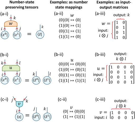
FIGURE 1. (a) An example of a number-state preserving tensor that w maps a number state ⟨z0|⟨z1| on its input indices to a number state
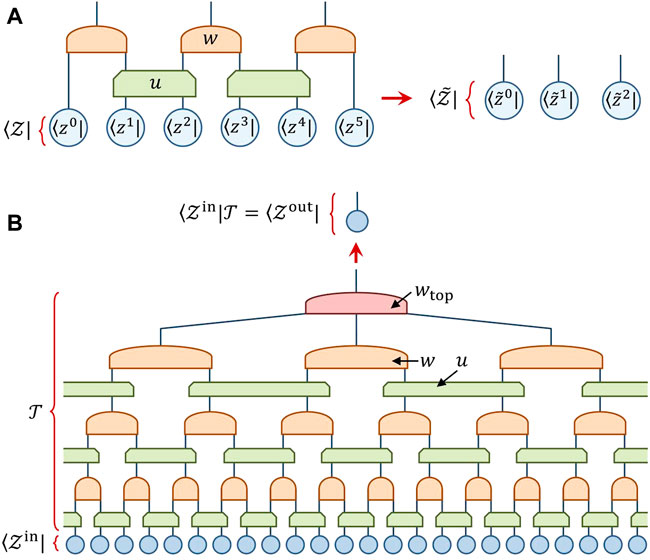
FIGURE 2. (A) A number-state preserving network is formed through composition of number-state preserving tensors u and w, which maps input number state
For the main text of this paper we shall further restrict our consideration to unital number-state preserving tensors, where each tensor entry must be either a zero or a one, and each row of the corresponding input-output matrix is required to have a single non-zero entry. Note that this class of tensor maps incoming number-states to outgoing number-states of the same normalization and phase. The restriction to unital tensors will be useful in simplifying their application to supervised learning problems, although the formalism and optimization algorithms that we present are still general for all number-state preserving networks. There are many reasons why one may also wish to consider networks comprised of non-unital number-state preserving tensors, where entries can take any real or complex value, and thus change the normalization of states and introduce phases; the interested reader is directed to Supplementary Appendix SA for further discussion.
Given that number-state preserving networks represent a severely restricted class of tensor network states it may be interesting to consider how much of their power has been lost, for instance, in describing ground states of quantum many-body systems. Although this remains to be explored, it seems likely that majority of many-body systems will not have ground-states that can be well-approximated by number-state preserving tensor networks. However, there does exist several examples of non-trivial quantum many-body systems related to Motzkin paths [43], whose ground states possess interesting entanglement and yet can be exactly represented by number-state preserving networks [44, 45]. Investigation of the ability of number-state preserving networks to describe general quantum ground states remains an intriguing direction for future research.
3 Supervised learning in a tensor product space
In this section we discuss how the task of supervised learning can be formulated in terms of tensor networks. We consider problems where each training sample
where k is a label over the set of training samples. Every training sample is assumed to be paired with a corresponding label
Although classifiers based on linear functions f have some considerable utility [46], many non-trivial classification problems require non-linear functions f in order to achieve good accuracy.
We now describe how a tensor network can be implemented as the classifying function in Eq. 4. At this point, one could be tempted to believe that tensor networks would have limited utility as classifiers as, given that tensors simply are extensions of matrices to higher dimensions, they are inherently linear constructs. However, in order to recast the supervised learning problem into a problem amenable to tensor networks, we first (non-linearly) embed the training data into a higher dimensional space, similar to a kernel method [47]. By using an appropriate non-linear embedding, a linear classifier acting the higher dimension space can reproduce the classifying power of non-linear functions in the original space; thus it remains possible that tensor network approaches could be competitive with classifiers based on (non-linear) neural networks. Indeed, as will be argued later in this manuscript, it can be understood that a tensor network of sufficiently large bond dimension χ can, in principle, obtain perfect accuracy for any training set of a supervised learning problem as formulated above.
Let us recast each training sample
Similarly the data labels yk are recast as number states |yk⟩ in a c-dimensional space. The diagrammatic tensor notation for these states is presented in Figure 3. Given this embedding of our training data, a classifier can be represented as tensor network
see also Figure 2B for an explicit example.

FIGURE 3. (A) The kth training sample
In general, the accuracy of
The diagrammatic tensor notation for Eq. 7, in the particular case that
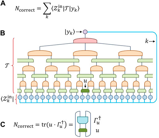
FIGURE 4. (A) The total number correctly classified samples Ncorrect is given as the inner product of the labels |yk⟩ against the network
Before moving on, we remark that the formalism we described (or similar formalisms consider previously [21, 23, 26–28, 31]) for addressing supervised learning problems using tensor networks could, in principle, employ arbitrary tensor networks
4 Single tensor updates
In this section we propose a method to optimize the tensors of a network
Key to this optimization strategy is the notion of a tensor environment, which can be understood as the derivative of the network with respect to a single tensor. Specifically, given a network that evaluates to a scalar such as that from Figure 4B, the environment Γu of a tensor u results from contracting the entire network sans the particular tensor u under consideration. It follows that the number of correctly classified samples Ncorrect from Eq. 7 can always be expressed as the scalar product of a tensor
where, for notational simplicity, we have recast u and Γu into input-output matrices, see Figure 4C. We relegate a description of the general method for computing environments Γu to Section 5 of the manuscript, and proceed here assuming Γu is already known.
Let us now turn to the problem of finding the optimal number-state preserving tensor uopt.,
which maximizes the number of correctly identified samples Ncorrect of Eq. 8, given a known environment Γu. Here it is easy to see that uopt. can be built by simply identifying the location of the maximal element in each row of Γu and then placing the unit element at the corresponding location in each row of uopt., with all other entries zero. Note that if the maximal element in a row of Γu is degenerate then uopt. is not uniquely defined; one can still obtain an optimal solution by simply selecting one of the maximal elements in that row of Γu. Let us consider a concrete example: imagine we are updating a tensor u with a 4 × 4 input-output matrix of the form given in Figure 1b-iii, and assume that the environment has been evaluated as
Then the (unital and number-state preserving) 4 × 4 matrix uopt. that maximizes Eq. 8 is given as
and the number of correctly classified training samples after this optimal update is given as Ncorrect = (12 + 9 + 22 + 15) = 58. Some remarks are in order regarding this optimization strategy. Firstly, we notice that unlike many commonly used algorithms for training neural networks, our approach is not based upon a gradient descent. Instead we can directly “hop” to the true maximum for any single tensor (given that the other tensors in the network are held remain fixed), provided the environment is exactly known. While this strategy has some advantages over gradient based methods with respect to avoiding local maxima, getting stuck in a solution that is not globally optimal can still remain a possibility depending on the problem until consideration.
We now discuss methods to introduce some randomness into the optimization, in order to reduce the possibility of getting trapped in a local maxima. One approach could be to employ a similar strategy as used in the stochastic gradient descent methods [49], where randomness is introduced by using only select “batch” of training samples for each update. Instead, here we advocate a different strategy inspired by Monte Carlo methods [50] used in sampling many-body systems. Rather than updating to the optimal tensor uopt. at each step, we propose to allow updates to sub-optimal solutions of Eq. 8, with a probability diminishes exponentially in relation to how far the solution is from the optimal solution. For this purpose we first introduce the difference matrix Ω, given by subtracting from each row of Γ the maximal element within the row,
For the example environment Γu given in Eq. 10 the corresponding difference matrix is
We then use the difference matrix to generate a matrix ptrans. of transition probabilities, defined element-wise as
where α is a tunable parameter that sets the amount of randomness. For the example difference matrix Ω of Eq. 13 and setting α = 2 we get the transition matrix
The transition matrix is then used to perform a stochastic update of the tensor u under consideration: values in each row of ptrans. set the probability for the unit element in the equivalent row of the updated u to be placed at that particular location (note that Eq. 14 has been defined such that each row of ptrans sums to unit probability). Notice that in the limit α → 0 the matrix ptrans. tends to uopt. (provided Γ had no degeneracies in its maximal row values), since all non-optimal transitions are fully suppressed. Conversely, in limit α → ∞ all probabilities in ptrans. tend to the same value, representing completely random transition probabilities.
5 Evaluation of tensor environments
Here we describe evaluation of tensor environments, crucial to the optimization algorithm discussed in the previous section. For simplicity, we describe this evaluation assuming the tensor network
Rather than tackling the problem of computing tensor environments Γ directly, we first introduce the concept of configuration spaces |ϕ⟩. Proper use of configuration spaces |ϕ⟩, which play an analogous role to the local reduced density matrices ρ used to optimize tensor networks in the context of quantum many-body systems, will greatly simplify the subsequent evaluation of environments. Let us assume that the output index of the tensor network
where the sum runs over all valid configurations σ of number states
An example of a network that could be contracted to evaluate a configuration space |ϕB⟩ is depicted in Figure 5A. It is seen that this network can be simplified, as shown Figure 5B, by lifting the input number state
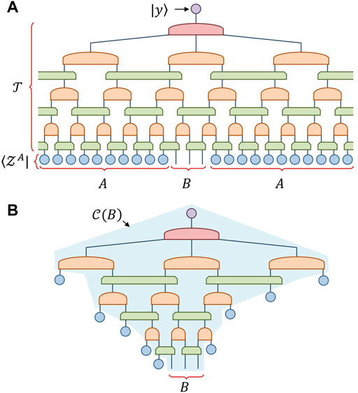
FIGURE 5. (A) The network
Notice that this configuration causal cone
The process of evaluating the configuration space for a region B of three sites from a binary MERA is depicted in Figure 6A. This evaluation can be formulated as a sequence of contractions that each “lower” the configuration space through the causal cone,
where bracketed subscripts denote configuration spaces at different depths within the network. Each of the lowering contractions is implemented by one of two geometrically different lowering operators, depicted in Figure 6B, which are the direct analogues to the descending superoperators [48] used in the evaluation of density matrices from isometric MERA.
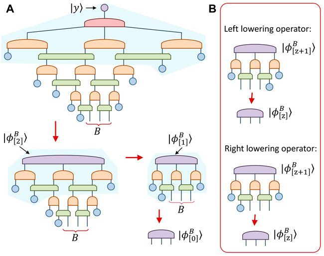
FIGURE 6. (A) Sequence of contractions used to evaluate the configuration space
In our example using a binary MERA, the cost of evaluating
Given that the evaluation of configuration spaces has been understood, we now turn to the task of building the environment Γu associated to tensor u, as depicted in Figure 7, which is accomplished as follows. First we lift the initial number state
see also Figure 7C.
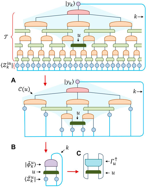
FIGURE 7. The sequence of steps used to evaluate the environment Γu of the shaded tensor u. (A) The initial state
6 Benchmark results
In this section we present benchmark results for how number-state preserving tensor networks perform as classifiers in some simple problems. The goal here is to establish the feasibility of our proposal, rather than to establish performance for challenging real-world tasks, which will be considered in future work. In particular we demonstrate 1) that the proposed optimization algorithms can efficiently and reliably train the networks under consideration, and 2) that number-preserving networks perform comparably well to unrestricted networks for classification tasks.
6.1 Parity classification
For this first test, we benchmark the performance of a number-state preserving MPS for classifying the parity of binary strings. Here each test sample is a length-N binary vector

FIGURE 8. (A) Tensor v is a number-state preserving tensor mapping from two indices to a single index. (B) An MPS network
A summary of the results from a large number of trials is presented in Table 1. For binary strings of length N = 16 and N = 20 we used 1,300 and 20,000 training samples respectively; these numbers were chosen as they represent about 2% of all possible binary strings in each case (of which there are 2N in total). The randomness parameter was fixed at α = 1 for N = 16 and α = 5 for N = 20 length chains; these values were determined as adequate through small amount of experimentation (and are probably not those which would give optimal performance). Somewhat surprisingly, we found that each trial would produce only one of two outcomes: 1) the optimization would fail completely, achieving only slightly over 50% classification accuracy on the set of all binary strings, or 2) would converge to a perfect parity classifier, with 100% classification accuracy for all length-N binary strings. From Table 1 we see the proportion nperfect of perfect classifiers obtained increases dramatically as the bond dimension χmax was increased, reaching 96/100 for N = 20 and χmax = 10. This is expected, as networks with more degrees of freedom are less likely to be trapped in local minima. We found that the likelihood of obtaining a perfect classifier was also greatly improved when using a larger number of training samples, although do not provide this data here. In a recent work by Stokes and Terilla [52] standard (unrestricted) MPS were also trained to classify the parity of binary strings, and produced comparable results for similar strings lengths and training set sizes. This is a good indication that, for this classification problem, number-state preserving MPS are as powerful as unrestricted MPS.
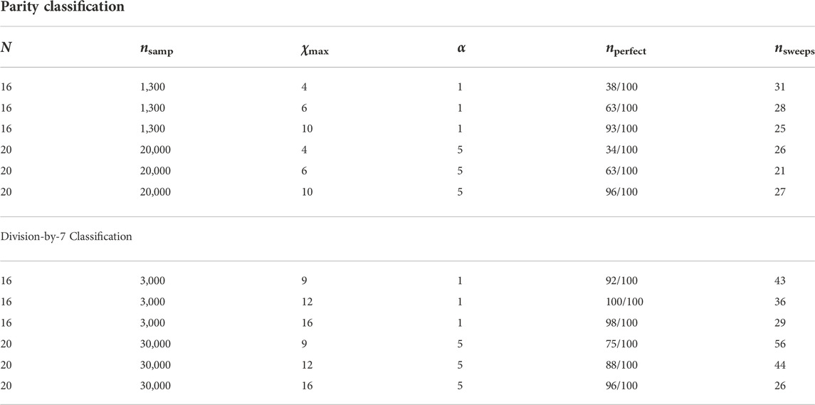
TABLE 1. Summary of results for MPS applied to the parity classification (above) and division-by-7 classification (below). Parameters are as follows: N is the length of binary strings classified, nsamp is the number of samples in the training set, χmax is the maximal MPS bond dimension, parameter α controls the randomness in the optimization as per Eq. 14, nperfect is the proportion of trial runs that yielded perfect (100% accuracy) classifiers, nsweeps is the average number of variational sweeps required to reach convergence.
6.2 Division-by-7 classification
For the second test we classify binary strings, interpreted as a base-2 representation of an integer, by their remainder under division by 7. We again use a number-state preserving MPS, employing the same set-up as used for the parity classification considered previously. A key difference here is that the samples now take one of seven different labels, yk ∈ {0, 1, 2, 3, 4, 5, 6}.
A summary of the results from these trials is presented in Table 1. For binary strings of length N = 16 and N = 20 we used 3,000 and 30,000 training samples, respectively; although this was more than was used for the parity classification it is still less than 5% of the possible binary strings. Similar to the parity benchmark, we here found that each trial would either fail completely, producing no better than a random results, or would converge to a perfect division classifier, with 100% classification accuracy for all length-N binary strings. As with the parity benchmark, it is seen that the proportion of perfect classifiers obtained increases steadily with the bond dimension χmax. However, this problem required larger dimensions χmax than used for the parity benchmark, which is expected since here we have many more classification categories.
6.3 Height classification
The final test problem that we consider, which we refer to as height classification, takes length-N strings of integers from the set z ∈ { − 1, 0, 1} and classifies them with labels yk ∈ {0, 1, 2} depending on whether the sum (under regular addition) of the integers is positive, zero or negative, respectively. We test the effectiveness of both number-state preserving binary TTN and binary MERA as classifiers for this problem, working with strings of length N = 24. A binary MERA of the form depicted in Figure 2B is used, and is compared with the binary TTN that would result from restricting to trivial disentanglers u throughout the MERA network. Given that the problem is translation-invariant, we imposed that all tensors within a network layer are identical. In terms of the optimization, this is achieved by updating using the average single-tensor environment from all equivalent tensors within a network layer. We found that the injection of randomness into the optimization was unnecessary, possibly due to the imposition of translational invariance, such that the randomness parameter α from Eq. 14 could be set at α = 0. This left the bond dimension of the networks as the only hyper-parameter in the calculation, which was fixed at maximum dimension χmax = 9.
The benchmark results are displayed in Figure 9, and consisted of 100 trials, each trial starting from 12,000 randomly generated training samples (with 4,000 samples from each label category) and a randomly initialized network. Rather than running separate TTN and MERA trials they were instead combined: the first 20 sweeps were performed with trivial disentanglers u, such that underlying the network was a TTN, the u were then “switched on” for the remaining 40 sweeps such that the network became a MERA. At the conclusion of each trial, the generalization error was estimated by applying the trained classifiers to a randomly generated test set of the same size as the training set. Most of the trials converged smoothly, with the proportion of wrongly identified testing samples decreasing monotonically with optimization, although about 5 trials failed to properly converge (yielding classifiers with greater than 30% error). Discarding the worst 10 trials from consideration, of the 90 remaining trials the TTN gave average training/test errors of 14.15% and 14.91%, while MERA gave substantially reduced average training/test errors of 1.13% and 1.86%. These results clearly demonstrate the extra representation power endowed through use of the disentanglers u in MERA. Impressive is that both networks generalized well, with only relatively small differences between test and training accuracies, despite being trained on less than 5 × 10⁻⁶ percent of the possible 324 training samples.
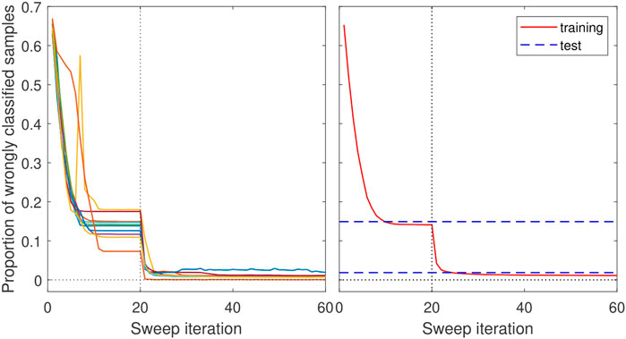
FIGURE 9. (left) Results of training TTN and MERA for the height classification problem, displaying how much of training set is wrongly classified as a function of the number of optimization sweeps performed. The first 20 sweeps are performed while keeping trivial disentanglers u, such that underlying the network is a TTN, while the u are then “switched on” for the remaining sweeps such that the network becomes a MERA. The figure displays results from 10 different trials, where each trial starts with a randomly generated training set and randomly initialized network. (right) Average results of the training data from 100 trial runs (after discarding the 10 worst trials). Dashed lines show the average generalization error computed from applying the trained TTN and MERA applied to a randomly generated test set. For TTN we get average training/test errors of 14.15% and 14.91%, while for MERA we get average training/test errors of 1.13% and 1.86%.
7 Conclusion
We have proposed the class of number-state preserving tensor networks for use as classifiers in supervised learning tasks and have shown that a large class of these networks, specifically those with bounded causal structure, are efficiently trainable for large problems. In particular we have described a training algorithm that, for any chosen tensor in the network under consideration, exactly identifies the optimal tensor for that location (i.e., that which maximizes the number of correctly classified training samples), all with cost that scales only linearly in number of training samples. Importantly, the class of efficiently trainable number-state preserving networks includes realizations of sophisticated networks such as MERA, which would otherwise be computationally intractable. As such, we believe this could be the first computationally viable proposal which would allow MERA, close tensor network analogues to convolutional neural networks, to be applied as classifiers for challenging tasks such as image recognition. This remains an interesting direction for future research.
Although number-state preserving tensors represent a highly restricted class of tensor, the preliminary results of Section 6 are encouraging that this class is sufficient when applying tensor networks as classifiers for learning problems as outlined in Section 3. It still remains to be seen whether number-state preserving tensor networks are as powerful as generic tensors networks for these tasks; this question requires further theoretical and numerical investigation. However it is relatively easy to understand that, in the limit of large bond dimension, a number-state preserving tensor network could in principle achieve 100% accuracy on any training problem outlined in Section 3. The reasoning follows similarly to the argument that a generic tensor network can represent an arbitrary quantum state in the limit of large bond dimension. Consider, for instance, the MERA depicted in Figure 2B. One could increase the bond dimension of indices within the network until the output index of each w tensor matches the product of its input dimensions, in which case each w could be fixed as a trivial identity tensor when viewed as an input-output matrix. In this scenario, the top tensor wtop could implement an arbitrary classifier that would perfectly map every training sample to its designated label, regardless of the training data given.
A major difficulty with the use of MERA in D = 2 or higher spatial dimensions [37, 38] is their high scaling of computational cost with bond dimension χ. However, there is reason to be more optimistic for their application as classifiers. The cost of contracting an isometric metric MERA for a density matrix, necessary for its optimization towards the ground state of a local Hamiltonian, is related to the size of the maximum causal width of the network. For instance, the most efficient known 2D isometric MERA [38] has a causal width of 2 × 2 sites, such that the density matrices within the causal cone have 8 indices. The cost of computing these density matrices can be shown to scale at most as O (χ16). However, while a number-state preserving version of this 2D MERA would also have a causal width of 2 × 2 sites, the relevant configuration space |ψ⟩ within the causal cone would only have 4 indices (which follows as the density matrix involves both the bra and the ket state, whereas the configuration space only involves the ket). Thus the cost of optimizing a number-state preserving version of this 2D MERA, where the key step is the evaluation of configuration spaces, will scale roughly as O (χ8) (i.e., the square-root of the cost of optimizing an isometric MERA for a quantum ground state). This square-root reduction in cost scaling as a function of bond dimension χ from isometric to number-state preserving networks will hold in general, such that number-state preserving networks could realize much larger bond dimensions given a fixed computational budget. This advantage is somewhat mitigated by the fact that the cost of optimizing a number-state preserving network comes with a factor nsamp related to the size of the training set, which could be very large. However, it would also be straight-forward to parallelize the evaluation of environments over the samples.
Although the main text of this manuscript focused on number-state preserving versions of MERA, many other forms of hierarchical network could also be of useful as classifiers as discussed further in Supplementary Appendix SB1. In particular the network of Supplementary Figure SB2, which does not have an isometric counterpart, seems to be the closest tensor network analogue to a convolutional neural network. Rather than disentanglers, this network uses δ-function tensors to effectively allow neighboring w tensors to “read” from the same boundary sites, mirroring the overlap of feature maps arising in a convolution (and similar to the generalized networks recently proposed in Ref. [31]). It would be interesting to compare the effectiveness of this structure versus a traditional MERA, which will be considered in future work.
Data availability statement
The original contributions presented in the study are included in the article/Supplementary Material, further inquiries can be directed to the corresponding author.
Author contributions
Manuscript is the singular effort of GE.
Funding
This research was supported in part by the National Science Foundation under Grant No. NSF PHY-1748958.
Acknowledgments
The author thanks Miles Stoudenmire and John Terilla for useful discussions and comments.
Conflict of interest
The author declares that the research was conducted in the absence of any commercial or financial relationships that could be construed as a potential conflict of interest.
Publisher’s note
All claims expressed in this article are solely those of the authors and do not necessarily represent those of their affiliated organizations, or those of the publisher, the editors and the reviewers. Any product that may be evaluated in this article, or claim that may be made by its manufacturer, is not guaranteed or endorsed by the publisher.
Supplementary Material
The Supplementary Material for this article can be found online at: https://www.frontiersin.org/articles/10.3389/fphy.2022.858388/full#supplementary-material
References
1. Carleo G, Cirac JI, Cranmer K, Daudet L, Schuld M, Tishby N, et al. Machine learning and the physical sciences. Rev Mod Phys (2019) 91:045002. doi:10.1103/RevModPhys.91.045002
2. Carrasquilla J, Melko RG. Machine learning phases of matter. Nat Phys (2017) 13:431–4. doi:10.1038/nphys4035
3. Broecker P, Carrasquilla J, Melko RG, Trebst S. Machine learning quantum phases of matter beyond the fermion sign problem. Sci Rep (2017) 7:8823. doi:10.1038/s41598-017-09098-0
4. Ch’ng K, Carrasquilla J, Melko RG, Khatami E. Machine learning phases of strongly correlated fermions. Phys Rev X (2017) 7:031038. doi:10.1103/physrevx.7.031038
5. Huembeli P, Dauphin A, Wittek P. Identifying quantum phase transitions with adversarial neural networks. Phys Rev B (2018) 97:134109. doi:10.1103/physrevb.97.134109
6. Liu Y-H, van Nieuwenburg EPL. Discriminative cooperative networks for detecting phase transitions. Phys Rev Lett (2018) 120:176401. doi:10.1103/physrevlett.120.176401
7. Canabarro A, Fanchini FF, Malvezzi AL, Pereira R, Chaves R. Unveiling phase transitions with machine learning. Phys Rev B (2019) 100:045129. doi:10.1103/PhysRevB.100.045129
8. Torlai G, Mazzola G, Carrasquilla J, Troyer M, Melko RG, Carleo G. Neural-network quantum state tomography. Nat Phys (2018) 14:447–50. doi:10.1038/s41567-018-0048-5
9. Carrasquilla J, Torlai G, Melko RG, Aolita L. Reconstructing quantum states with generative models. Nat Mach Intell (2019) 1:155–61. doi:10.1038/s42256-019-0028-1
10. Torlai G, Melko RG. Learning thermodynamics with Boltzmann machines. Phys Rev B (2016) 94:165134. doi:10.1103/physrevb.94.165134
11. Carleo G, Troyer M. Solving the quantum many-body problem with artificial neural networks. Science (2017) 355:602–6. doi:10.1126/science.aag2302
12. Choo K, Neupert T, Carleo G. Study of the two-dimensional frustrated J1-J2 model with neural network quantum states. Phys Rev B (2019) 100:125124. doi:10.1103/PhysRevB.100.125124
15. Orús R. A practical introduction to tensor networks: Matrix product states and projected entangled pair states. Ann Phys (N Y) (2014) 349:117–58. doi:10.1016/j.aop.2014.06.013
16. Levine Y, Sharir O, Cohen N, Shashua A. Quantum Entanglement in Deep Learning Architectures. Phys Rev Lett (2019) 122:065301. doi:10.1103/PhysRevLett.122.065301
17. Huang Y, Moore JE. Neural network representation of tensor network and chiral states. Phys Rev Lett (2021) 127:170601. doi:10.1103/PhysRevLett.127.170601
18. Deng D-L, Li X, Das Sarma S. Quantum entanglement in neural network states. Phys Rev X (2017) 7:021021. doi:10.1103/physrevx.7.021021
19. Glasser I, Pancotti N, August M, Rodriguez ID, Cirac JI. Neural-network quantum states, string-bond states, and chiral topological states. Phys Rev X (2018) 8:011006. doi:10.1103/physrevx.8.011006
20. Cai Z, Liu J. Approximating quantum many-body wave functions using artificial neural networks. Phys Rev B (2018) 97:035116. doi:10.1103/physrevb.97.035116
21. Stoudenmire EM, Schwab DJ. Supervised learning with quantum-inspired tensor networks. Adv Neural Inf Process Syst (2016) 29:4799. doi:10.48550/arXiv.1605.05775
22. Cohen N, Sharir O, Levine Y, Tamari R, Yakira D, Shashua A. Analysis and design of convolutional networks via hierarchical tensor decompositions. arXiv:1705.02302 (2017). doi:10.48550/arXiv.1705.02302
23. Han Z-Y, Wang J, Fan H, Wang L, Zhang P. Unsupervised generative modeling using matrix product states. Phys Rev X (2018) 8:031012. doi:10.1103/PhysRevX.8.031012
24. Cichocki A, Phan A-H, Zhao Q, Lee N, Oseledets I, Sugiyama M, et al. Tensor networks for dimensionality reduction and large-scale optimization: Part 2 applications and future perspectives. FNT Machine Learn (2017) 9:249–429. doi:10.1561/2200000067
25. Liu D, Ran S-J, Wittek P, Peng C, Garca RB, Su G, et al. Machine learning by two-dimensional hierarchical tensor networks: A quantum information theoretic perspective on deep architectures. New J Phys (2019) 21:073059. doi:10.1088/1367-2630/ab31ef
26. Hallam A, Grant E, Stojevic V, Severini S, Green AG. Compact neural networks based on the multiscale entanglement renormalization ansatz. arXiv:1711.03357 (2017). doi:10.48550/arXiv.1711.03357
27. Stoudenmire EM. Learning relevant features of data with multi-scale tensor networks. Quan Sci Technol (2018) 3:034003. doi:10.1088/2058-9565/aaba1a
28. Liu Y, Li W-J, Zhang X, Lewenstein M, Su G, Ran S-J. Entanglement-Based Feature Extraction by Tensor Network Machine Learning. Front Appl Math Stat (2021). doi:10.3389/fams.2021.716044
29. Huggins W, Patel P, Whaley KB, Stoudenmire EM. Towards quantum machine learning with tensor networks. Quan Sci Technol (2019) 4:024001. doi:10.1088/2058-9565/aaea94
30. Grant E, Benedetti M, Cao S, Hallam A, Lockhart J, Stojevic V, et al. Hierarchical quantum classifiers. npj Quan Info (2018) 4:65. doi:10.1038/s41534-018-0116-9
31. Glasser I, Pancotti N, Cirac JI. From probabilistic graphical models to generalized tensor networks for supervised learning. arXiv:1806.05964v2 (2018). doi:10.48550/arXiv.1806.05964
32. Fannes M, Nachtergaele B, Werner RF. Finitely correlated states on quantum spin chains. Commun Math Phys (1992) 144:443–90. doi:10.1007/bf02099178
33. Ostlund S, Rommer S. Thermodynamic limit of density matrix renormalization. Phys Rev Lett (1995) 75:3537–40. doi:10.1103/physrevlett.75.3537
34. Shi Y, Duan L, Vidal G. Classical simulation of quantum many-body systems with a tree tensor network. Phys Rev A (Coll Park) (2006) 74:022320. doi:10.1103/physreva.74.022320
35. Tagliacozzo L, Evenbly G, Vidal G. Simulation of two-dimensional quantum systems using a tree tensor network that exploits the entropic area law. Phys Rev B (2009) 80:235127. doi:10.1103/physrevb.80.235127
36. Vidal G. Class of quantum many-body states that can Be efficiently simulated. Phys Rev Lett (2008) 101:110501. doi:10.1103/physrevlett.101.110501
37. Cincio L, Dziarmaga J, Rams MM. Multiscale entanglement renormalization ansatz in two dimensions: Quantum ising model. Phys Rev Lett (2008) 100:240603. doi:10.1103/physrevlett.100.240603
38. Evenbly G, Vidal G. Entanglement renormalization in two spatial dimensions. Phys Rev Lett (2009) 102:180406. doi:10.1103/physrevlett.102.180406
39. Evenbly G, Vidal G. Quantum criticality with the multi-scale entanglement renormalization ansatz, chapter 4 in strongly correlated systems: Numerical methods. In: A Avella,, and F Mancini, editors. Springer Series in Solid-State Sciences (2013).
40. LeCun Y, Boser B, Denker JS, Henderson D, Howard RE, Hubbard W, et al. Backpropagation applied to handwritten zip code recognition. Neural Comput (1989) 1(4):541–51. doi:10.1162/neco.1989.1.4.541
41. Krizhevsky A, Sutskever I, Hinton GE. ImageNet classification with deep convolutional neural networks. Commun ACM (2017) 60(6):84–90. doi:10.1145/3065386
42. Simonyan K, Zisserman A. Very deep convolutional networks for large-scale image recognition. arXiv:1409.1556 (2014). doi:10.48550/arXiv.1409.1556
43. Bravyi S, Caha L, Movassagh R, Nagaj D, Shor P. Criticality without frustration for quantum spin-1 chains. Phys Rev Lett (2012) 109:207202. doi:10.1103/physrevlett.109.207202
44. Alexander RN, Evenbly G, Klich I. Exact holographic tensor networks for the Motzkin spin chain. Quan (2021) 5:546. doi:10.22331/q-2021-09-21-546
45. Alexander RN, Ahmadain A, Klich I. Holographic rainbow networks for colorful Motzkin and Fredkin spin chains. Phys Rev B (2019) 100:214430. doi:10.1103/PhysRevB.100.214430
46. Yuan G-X, Ho C-H, Lin C-J. Recent advances of large-scale linear classification. Proc IEEE (2012) 100(9):2584–603. doi:10.1109/jproc.2012.2188013
47. Hofmann T, Schölkopf B, Smola AJ. Kernel methods in machine learning. Ann Statist (2008) 36:1171. doi:10.1214/009053607000000677
48. Evenbly G, Vidal G. Algorithms for entanglement renormalization. Phys Rev B (2009) 79:144108. doi:10.1103/physrevb.79.144108
49. Zhang T. Solving large-scale linear prediction problems with stochastic gradient descent. In: Proceedings of the international conference on machine learning (2004).
50. Metropolis N, Rosenbluth AW, Rosenbluth MN, Teller AH, Teller E. Equation of state calculations by fast computing machines. J Chem Phys (1953) 21:1087–92. doi:10.1063/1.1699114
51. Evenbly G, Vidal G. Scaling of entanglement entropy in the (branching) multi-scale entanglement renormalization ansatz. Phys Rev B (2014) 89:235113. doi:10.1103/physrevb.89.235113
Keywords: tensor network, machine learning, matrix product ansatz, quantum many body theory, numerical optimization
Citation: Evenbly G (2022) Number-state preserving tensor networks as classifiers for supervised learning. Front. Phys. 10:858388. doi: 10.3389/fphy.2022.858388
Received: 19 January 2022; Accepted: 25 October 2022;
Published: 29 November 2022.
Edited by:
Peng Zhang, Tianjin University, ChinaReviewed by:
Sayantan Choudhury, Shree Guru Gobind Singh Tricentenary (SGT) University, IndiaDing Liu, Tianjin Polytechnic University, China
Shi-Ju Ran, Capital Normal University, China
Copyright © 2022 Evenbly. This is an open-access article distributed under the terms of the Creative Commons Attribution License (CC BY). The use, distribution or reproduction in other forums is permitted, provided the original author(s) and the copyright owner(s) are credited and that the original publication in this journal is cited, in accordance with accepted academic practice. No use, distribution or reproduction is permitted which does not comply with these terms.
*Correspondence: Glen Evenbly, Z2xlbi5ldmVuYmx5QGdtYWlsLmNvbQ==
 Glen Evenbly