Data-Driven State Fragility Index Measurement Through Classification Methods

As environmental changes cause a series of complex issues and unstable situation, exploring the impact of environmental changes is essential for national stability, which is helpful for early warning and provides guidance solutions for a country. The existing mainstream metric of national stability is the Fragile States Index, which includes many indicators such as abstract concepts and qualitative indicators by experts. In addition, these indicators may have preferences and bias because some data sources come from unreliable platforms; it may not reflect the real situation for the current status of countries. In this article, we propose a method based on ensemble learning, named CR, which can be obtained by quantifiable indicators to reflect national stability. Compared with the current mainstream methods, our proposed CR method highlights quantitative factors and reduces qualitative factors, which is an advantage of simplicity and interoperability. The extensive experimental results show a significant improvement over the SOTA methods (7.13% improvement in accuracy, 2.02% improvement in correlation).

1 Introduction

In recent years, tremendous scientific outcomes have proved that environmental changes cause a considerable impact on the development of human society, and it shows different degrees of influence in different regions. As early as the end of the 20th century, many countries have begun to pay attention to research on the impact of environmental changes on the country’s economic and political stability, take measures to contain the speed of environmental changes, and respond to subsequent effects. In addition, at the beginning of the 21st century, the U.S. Department of Defense identified unstable factors related to the environment as a primary strategic consideration. Evidence shows that environmental pressure is an essential factor in contemporary conflicts [1]. It also shows that the conflicts caused by the environment are inspired by dynamic, complex, and interactive processes, not just a simple and deterministic relationship. Therefore, it is necessary to establish an analytical framework to understand the antecedents and consequences [35].

Environmental changes may lead to fatal results. Drastic changes in the environment will cause a series of humanitarian disasters, such as political violence, which makes an already fragile country worse off [2–4]. The urgent need and competition for limited resources such as energy, food, and water may rise to national military confrontation, thus causing a series of humanitarian disasters and political violence [5]. Environmental pressures caused by environmental changes are generally combined with weak governance and social divisions, thereby exacerbating national stability [6–9]. Therefore, it is insightful to mine association rules from existing data and evaluate the impact of environmental changes on national stability [10].

Besides, many metrics could evaluate national stability such as the Country Indicators for Foreign Policy (CIFP) [11] published by Carleton University and The Peace and Conflict Instability Ledger (PCIL) [12] compiled by the University of Maryland. The most widely used and well-performing metric is the Fragile States Index (FSI) [13] published annually by the American Bimonthly Foreign Policy and The Fund for Peace. The Fragile States Index consists of many indicators such as economic, military, politics, and society. And each indicator is obtained through the process of quantitative resource and qualitative evaluation by experts. However, the design of the Fragile State Index is complicated, and the concept used in evaluating the value of the indicator is abstract, which is not convenient for research and analysis. Specifically, in content analysis, there is a data preference for countries with sound volume, which may not reflect the real situation of some fragile countries. In the process of qualitative review by experts, there may also be subjective tendencies or stereotypes, making the value of the indicator unable to express accurately.

Ensemble learning is a learning algorithm. It utilizes multiple classifiers to combine to handle a more powerful performance [14,15]. Multiple classifiers through ensembles will generally perform better than a single classifier. Taking our daily life as an example, the social division of labor cooperation is a powerful way to improve work efficiency. By giving full care to individual strengths, individuals with different strengths are brought together to make them play a greater role. This is where the idea of ensemble learning comes from.

In this work, we study how to utilize quantitative ways to pursue reasonable ranking to measure national stability, which has certain similarity and high correlation with the FSI ranking. Our proposed CR method mainly involves label by stage division, machine learning methods for experiments, and ranking aggregation under the best method at each stage. The main contributions of our work are as follows: 1) We propose a new method based on the idea of ensemble learning, which applies different classifiers to aggregate the optimal classifier under different stages to achieve better prediction performance. 2) Combining the advantages of multiple machine learning methods with the idea of ensemble learning enables our method to obtain more valuable and insightful information, which enables our CR method universality. 3) Through a large number of experiments, our results show that ranking obtained by our proposed CR method is in line with the actual situation of the current national stability; it pays more attention to the quantification of the original data and reduces the impact of abstract indicators on the prediction performance, which makes it more quantifiable and interpretable.

2 Materials and Methods

In this section, we present our datasets and briefly introduce the classification methods. The classification methods could be divided into traditional machine learning and neural network methods.

2.1 Data

Our data resources are obtained from the World Bank,¹ Germanwatch,² The Fund for Peace,³ the International Trade Organization,⁴ and the Belt and Road Initiative.⁵ The descriptions of the data resources are as follows:

• Improved water, carbon emissions, and cultivated land: It is obtained from the World Bank and Germanwatch. Specifically, records per capita improved water of 236 countries from 2000 to 2015, the per capita carbon emissions (metric tons per capita) of 242 countries from 2000 to 2014, and the per capita cultivated land (hectares per capita) of 178 countries from 2007 to 2015. Improved water resources are not only related to the national investment but also to the harshness of the climate. (The percentage of per capita improved water in developed countries is generally higher.) And carbon emissions are a useful indicator for demonstrating a country’s industrial development. Cultivated land is a basis for agricultural production, and it is also an essential indicator for the country’s productivity. The changes in these indicators will have a great impact on the politics, economy, and society of the region.

• Climate Risk Index: It is collected from The Fund for Peace, which records the annual Global Climate Risk Index (CRI [16]) of 187 countries from 2007 to 2014. The CRI aims to analyze the extent to which countries and regions are affected by extreme weather loss events (storms, floods, heat waves, etc.). Regarding future climate change, the CRI may become a warning signal. Thus, it is considered a factor affecting environmental changes.

• International Trade Network: We obtained international trade network data from the International Trade Organization, which records the export trade status of 786 commodities in 192 countries/regions from 2001 to 2015. The international trade network data can well reflect the economic vitality and productivity of the region. The fitness and complexity algorithm was proposed by the authors of the study mentioned in reference [17], which aims to measure the economic health of a country and is a correct and simple way to measure the competitiveness of a country. Because of its outstanding performance in national economic forecasts, it was adopted by the World Bank in 2017. In the study, we examined the international trade network to apply the algorithm to calculate a fitness value to reflect the economic vitality and productivity of the country.

• The Belt and Road (B&R): We obtained data from the Belt and Road Initiative. Politics is also an important factor for affecting national stability; we set up a new feature to indicate whether a country belongs to the Belt and Road (B&R) initiative. B&R aims to actively develop economic and cultural exchanges with countries along the route [18]. At present, there are 65 countries and regions along with the Belt and Road Initiative, including 10 ASEAN countries, 8 South Asian countries, 5 Central Asian countries, 18 west Asian countries, 7 Commonwealth of Independent States countries, and 16 central and eastern European countries. Most of them are still developing countries.

• Continent: The continent is geographic data. Geography is important to a country’s development. It is the reason for great differences in economy, politics, society, and culture among different continents, especially in economic development.

2.2 Benchmark and Baseline Methods

2.2.1 Benchmark

The Fragile States Index (FSI, [13]) is a well-known ranking for evaluating national stability, which is published annually by the American Bimonthly Foreign Policy and The Fund for Peace. The FSI consists of 12 indicators in four aspects: economics, military, politics, and society. The score of each index ranges from 0 to 10, where 0 represents the most stable and 10 represents the least stable, thus forming a score spanning the scale of 0–120. The scores of each indicator are obtained through the process of content analysis (CAST) [19], quantitative resource, and qualitative evaluation by experts. Therefore, the most significant value of FSI is to rank and classify different countries and give different degrees of suggestions to different countries, so that they can better prepare for emergencies [11,20]. In this study, we use FSI ranking as our proposed CR method’s benchmark.

2.2.2 Baseline Methods

To evaluate our proposed CR method, we compare with two groups of baselines including traditional machine learning and neural network methods.

1) Traditional Machine Learning

• Support vector machine (SVM, [21]) is a powerful method for nonlinear problems. Its decision boundary is the maximum margin hyperplane to be solved for the learning sample.

• Decision tree: Decision tree (DT, [22]) is a widely used non-parametric supervised algorithm, which can be used for classification and regression problems. The decision tree simulates people’s decision-making process and makes predictions by deriving simple decision rules from samples.

• Random forest: Random forest (RF, [23]) is an algorithm based on ensemble learning, which is composed of decision tree and bagging. It utilized multiple decision trees to train the samples in parallel and then integrate them to form a forest to enhance the classification effect and generalization ability.

• Gradient boost decision tree (GBDT [22]) is also an ensemble learning algorithm, which is composed of many decision trees. GBDT can deal with all kinds of data flexibly and has good prediction performance.

• Extreme gradient boosting (XGBoost [24]) is essentially a GBDT, but it has made many improvements to the GBDT algorithm, which greatly improves the speed and efficiency of training. Compared with GBDT, XGBoost adds a regular term to the cost function, which makes the algorithm simpler. In addition, XGBoost utilizes the method of the random forest to support column sampling, which can not only alleviate the overfitting but also reduce the calculation.

• CatBoost, proposed by [25], is a machine learning method based on gradient boosting over decision trees with the aim to deal with the category characteristics efficiently. Currently, CatBoost can be widely used in a variety of fields and problems. It does not need too many tuning parameters to get strong performance and can effectively prevent overfitting, which also makes the model robust. But it takes a lot of memory and time to process the categorical features.

• NGBoost was proposed by [26]. It is a boosting method based on natural gradients. This method can directly get the full probability distribution in output space, which can be used for probability prediction to quantify uncertainty. It aims to solve the problem of general probabilistic prediction which is difficult to be handled by existing gradient promotion methods. Currently, NGBoost prediction is much more competitive than other boosting methods.

2) Neural Network

• Multi-layer perceptron (MLP, [27]), which is composed of an input layer, a hidden layer, and an output layer, is a simple neural network and the basis of other neural network structures.

• Convolutional neural network (CNN, [28]) is a feedforward neural network, which is one of the representative methods of deep learning. It usually includes a convolution layer, pooling layer, and full connection layer. CNN can share convolution kernel globally and process high-dimensional data.

• Long short-term memory (LSTM) [29] is a kind of recurrent neural network. Compared with the general neural network, it can deal with the data of sequence change. It aims to solve the problem of gradient disappearance and gradient explosion during long sequence training.

• Gated recurrent unit (GRU), proposed by [30], is similar to the basic concept and regarded as a variant of LSTM. The GRU has a simpler structure than LSTM, and it is faster to learn and train in data matching.

• Model-agnostic meta-learning (MAML) was proposed by [31]. It is a method based on meta-learning. MAML is used to adjust the initial parameters by one or more steps, and it achieves the goal of quickly adapting to a new task with only a small amount of data.

3 Proposed CR Method

In this section, we introduce our proposed CR method, which is based on the idea of ensemble learning. Due to each classification method is learned by data-driven which has its specific for feature selection. We choose the best classification method under different features and aggregate their predicted results to obtain better prediction results.

3.1 Stage Division

In essence, machine learning is a data-driven inductive bias method, that is, obtaining general knowledge from limited known data. Therefore, different classification methods may have different induction preferences, and the predicted results may also be different. First, we input the data into our method, which include features and labels. Next, we have the following steps: 1) The label of the input data is divided into N stages according to ranking with a certain ratio. 2) The input data are applied to various machine learning methods, and we can observe the best method performance under each stage. 3) The method and result with the best performance under each stage are chosen.

3.2 Ranking Aggregation

We chose the optimal method for each stage, and the optimal ranking of each stage can be obtained. But we cannot simply aggregate them because the problem of information interference will influence the final results. It is necessary to improve the robustness of aggregate ranking. In our method, we apply the Borda count method to aggregate the ranking. The Borda count method [32] is a traditional ranking aggregation method. Its main idea is to get a score for each element of each ranking list, which measures the gap between that element and other elements. Then, adding the scores of each element in the list produces a Borda number for each element. The ranking aggregation process is as follows:

$R_t=\sum _{j\left(j\ne i\right)}\left(r_{ti}-r_{tj}\right),(1)$

where r_ti denotes the rank of element t in the i-th position. By ranking the Borda number of elements, the final ranking results are obtained.

Ranking aggregation is better than the results given by a single classification method because it can take advantage of each method and aggregate them; it is an implementation of ensemble learning for ideas. The application of the Borda count method for our method is necessary; the method can smooth the samples that predict errors in each stage during the aggregation process. Therefore, it enables our method to have strong anti-interference and universality, which improves the robustness.

4 Experiments

To verify the effectiveness of our model, we conducted experiments on real data to evaluate national stability.

4.1 Evaluation Metrics

• Pearson correlation coefficient (PCC, [33]) is used to measure the degree of linear correlation between the two features of data α and β. According to the Cauchy–Schwarz inequality, the PCCs range from −1 to +1. Specifically, 1 represents the total positive linear correlation between the two features, 0 represents the wireless correlation, and −1 represents the total negative linear correlation between the two features. It is currently the most commonly used method to analyze the distribution trend and change trend consistency of the two sets of data and is widely used in the scientific field. The expression formula is as follows:

${\rho }_{X,Y}=\frac{\mathrm{c}\mathrm{o}\mathrm{v}\left(X,Y\right)}{{\sigma }_X{\sigma }_Y}=\frac{\left.\mathrm{E}\left[X-{\mu }_X\right)\left(Y-{\mu }_Y\right)\right]}{{\sigma }_X{\sigma }_Y}.(2)$

• Accuracy (ACC, [34]) refers to the proportion of correctly classified samples to the total samples. It does not consider whether the predicted samples are positive or negative. ACC is the most common metric. According to the results, the higher the ACC, the better will be the classifier. The expression formula is as follows:

$\text{\hspace{0.17em}ACC\hspace{0.17em}}=\frac{T_P+T_N}{T_P+T_N+F_P+F_N},(3)$

where T_P means that positive samples are correctly predicted as positive, T_N means that negative samples are correctly predicted as negative, F_P means that negative samples are incorrectly predicted as positive, and F_N means that positive samples are incorrectly predicted as negative.

In brief, ACC represents the precision of absolute ranking, while the PCCs represent the precision of relative ranking. We choose these two metrics to evaluate the results from different facets.

4.2 Experimental Settings

Since the collected datasets cover different years and the number of countries included, to facilitate subsequent calculations, data cleaning will be performed on all sample countries and years. Therefore, we removed the countries with missing data and took the intersection of the remaining by year and country. Finally, we split the data resources from 2010 to 2014 of 122 countries, comprising a total of 610 rows, with each piece of data containing 7 features including improved water, carbon emissions, cultivated land, Climate Risk Index, International Trade Network, B&R, continent, and FSI ranking as labels. All features are shown in Figure 1 and Figure 2. Then we utilize the data from 2010 to 2013 as the training set and the data from 2014 as the test set for verification. This experiment was run on a server with 1 NVIDIA Tesla V100 GPU. The operating system is Centos 7.5, and all the codes are implemented in the Python environment. The parameter settings are listed in Supplemental Data.

FIGURE 1

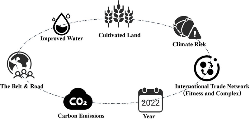
FIGURE 1. Data description. Each piece of data contains 8 features.

FIGURE 2

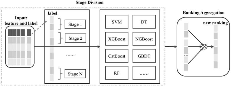
FIGURE 2. Overview of the CR framework.

4.3 Results on Classification Task

To explore the most effective machine learning algorithm for classification, we divide the status of the country into three stages based on the ranking of the FSI: fragile, warning, and stable, with a ratio of 3:4:3. Specifically, the countries ranked from 1 to 37 are fragile, the countries ranked from 38 to 86 are warning, and the countries ranked from 87 to 122 countries are stable. Then, we use 7 features as input, the country’s status as label, and ACC and PCCs as evaluation metrics. We use traditional machine learning and neural network methods to make predictions. The results are shown in Table 1.

TABLE 1

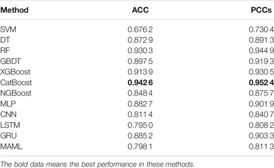
TABLE 1. Results of status classification. The data in bold represent the best performances in these methods.

Taking the results in Table 1, we have the following observations. On the whole, nearly half of the methods have ACC and PCCs above 0.9. It is demonstrated that the CatBoost method performance is the best; its ACC is achieved as high as 0.9426 and PCC as high as 0.9524. In terms of methods, traditional machine learning methods perform more prominently, especially CatBoost and RF methods based on ensemble learning (two of the best performances in all evaluation metrics). In the neural network methods, only MLP and GRU reach the general level, while LSTM and MAML do not perform well. The performance of each method is shown in Figure 3.

FIGURE 3

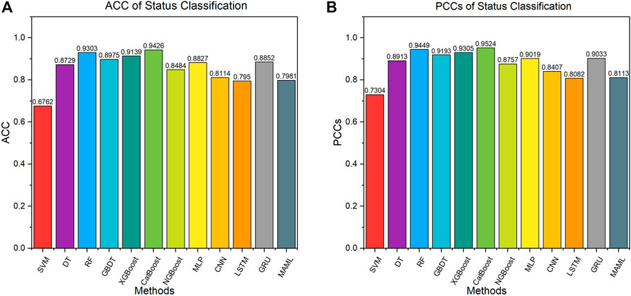
FIGURE 3. Result of status classifications. (A) ACC of status classification. (B) PCCs of status classification

4.4 Results on Ranking Task

Based on the result of status classification, we found that using classification methods can achieve good prediction performance. Thus, we propose an idea—ranking by classification. It uses classification methods to solve the ranking problem. We can continue to explore the prediction accuracy of each model under the label for FSI ranking. In addition, we can also observe the pros and cons of different methods in different countries’ status.

From the results given in Table 2, we have the following observations: In general, the ACC and PCCs of different methods at different stages are inconsistent, which means that different methods have different preferences for data fitting. For example, in the fragile stage, the ACC and PCCs of RF are not as good as CatBoost, but the RF’s performance in the stable stage is indeed much higher than the performance of other methods. This shows that in our task, RF predicts the lower ranked (stable) countries more accurately. In terms of methods, CatBoost and RF are still the best performing methods. In the fragile stage, the highest performing method for ACC and PCCs is CatBoost. In the warning stage, the best performance of ACC is achieved using CatBoost, and the best performance of PCCs is with RF. In the stable stage, the best performance is achieved using RF. Besides, both ACC and PCCs of the neural network–based MAML show that the performance is better than other neural network methods. This demonstrates that in our small data sample, MAML can also have its own advantages in small sample learning. However, compared with methods based on ensemble learning, neural networks appear a serious overfitting phenomenon in our task, which may be caused by too little data. It also demonstrates that traditional machine learning methods can still perform well in small datasets. We compared the top three methods of evaluation metrics at each stage and drew scatter charts to more intuitively indicate the similarity between the rankings. The results are shown in Figures 4A–F; Figure 5.

TABLE 2

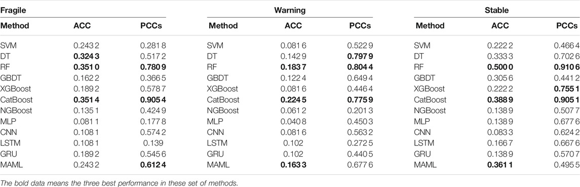
TABLE 2. Results of methods under different stages: fragile, warning, and stable. The data in bold represent the top three performances in these methods.

FIGURE 4

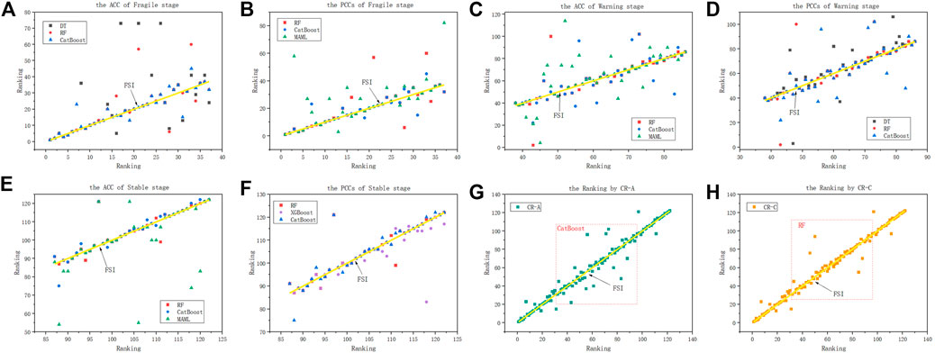
FIGURE 4. (A–F) Ranking of different methods in different stages. (G) Ranking obtained by the ACC-based CR method. (H) Ranking obtained by the PCC-based CR method.

FIGURE 5

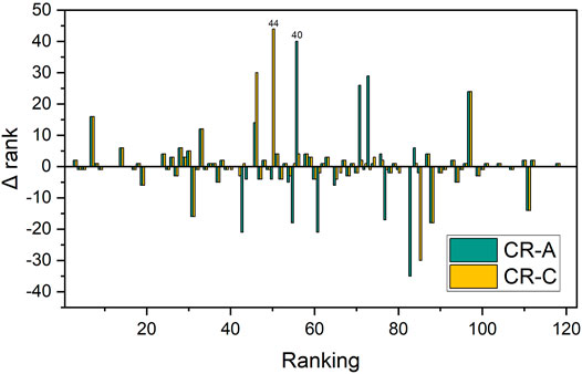
FIGURE 5. Difference between CR ranking and FSI ranking. The Δ rank represents the error value between CR ranking and FSI ranking. The error value is obtained by subtracting the FSI ranking from the CR ranking.

Based on the aforementioned observation, we utilized the idea of ensemble learning to aggregate the optimal methods at each stage, which will be an effective ranking method. We choose the method with the highest evaluation metrics for each stage. According to different metrics, we can get one method based on ACC, named CR-A, and another method based on PCCs, named CR-C. The CR-A method is composed of CatBoost-CatBoost-RF, which is the method that achieved highest ACC in each stage, and the CR-C method is composed of CatBoost-RF-RF, which is the method that achieved the highest PCCs in each stage.

For comparison, we used the FSI ranking as label and then utilized traditional machine learning and neural network methods for modeling and comparison with the CR method. The results are given in Table 3.

TABLE 3

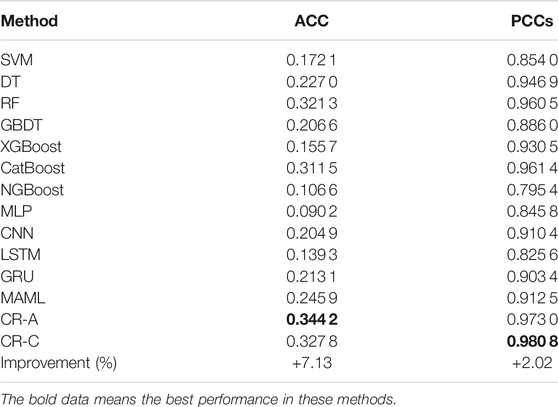
TABLE 3. Results of ranking comparison. The data in bold represent the best performances in these methods.

Taking the results in Table 3, it is demonstrated that our method consistently outperforms baseline in terms of ACC and PCCs. Specifically, CR-A outperforms the baseline methods for ACC (7.13% improvement), while CR-C outperforms the baseline methods for PCCs (2.02% improvement). This illustrates the effectiveness of our method based on the idea of ensemble learning. It is probably because it utilizes the idea of ensemble learning to aggregate the best learning methods at each stage that can deeply fit the data, which improves the prediction accuracy and correlation coefficient.

Next, we explore the difference between CR-A and CR-C methods. In order to observe more intuitively, we use scatterplots to show the ranking obtained by two methods, and the result is shown in Figures 4G,H. In addition, we use Δ rank to represent the ranking error value. The expression formula is as follows:

$\mathrm{\Delta }ran{k}_i=rank{\left(A\right)}_i-rank{\left(B\right)}_i,(4)$

where i represents an item, A and B represent different ranking methods, rank(A)_i is the ranking of item i under method A, and rank(B)_i is the ranking of item i under method B.

Considering the results in Figures 4G,H, we observe that the difference between the two methods is mainly due to the slightly larger difference in rankings in the middle segment. The CR-A method has a small error value (use Δ rank to indicate) in ranking fluctuations, but the number of error rankings is large. While the CR-C method gets a larger Δ rank in the fluctuation of a ranking, but the number of error rankings is small.

In order to understand the difference between the two methods more clearly, we calculate the Δ rank between the CR ranking and FSI ranking. As shown in 5, the maximum Δ rank of CR-A is 40, but there are 13 error rankings with Δ rank greater than 10, and 6 error rankings with Δ rank greater than 20. The CR-C has a maximum Δ rank of 44, but there are only 9 error rankings with Δ rank greater than 10, and 4 error rankings with Δ rank greater than 20. We found that the rankings obtained by the two methods are highly convergent with FSI ranking, and they all have their own advantages. The results of ranking by CR-A and CR-C are shown in Supplemental Data.

5 Discussion

This work mainly focuses on quantitative data to obtain a new ranking that is similar to the FSI ranking. In this study, we propose a new method—CR, based on the idea of ensemble learning. We examined stage division for labels, which utilizes some classifiers to extract complex patterns from features in each stage and aggregates the best performing ranking from each stage. Compared with the FSI, our method pays more attention to the quantification of ways, reducing the impact of abstract factors and expert qualitative indicators, which makes the new ranking more quantitative and interpretable. The experimental results show that our method is able to improve both accuracy and coefficient compared to the state-of-the-art methods.

In our experiment, we compared few traditional machine learning and neural network methods, but the results show that the prediction effect of the neural network is not as good as traditional machine learning, especially methods based on ensemble learning. The possible reason is that for the small sample data, the neural network is prone to overfitting so that it cannot perform excellent generalization performance. In addition, the experimental results also demonstrate that ensemble learning methods such as CatBoost and RF are more suitable for our work. One interesting future direction of this work is to adopt brain drain and electrical energy, which improve the method from balancing robust and accuracy.

Data Availability Statement

The original contributions presented in the study are included in the article/Supplementary Material; further inquiries can be directed to the corresponding authors.

Author Contributions

XL and HL contributed to conceptualization, methodology, and writing—original draft preparation. XL helped with data generating and collection. XL and HL assisted with experiments and discussions. XL, AV, HL, and KL involved in writing—reviewing and editing.

Funding

We acknowledge the financial support from the National Natural Science Foundation of China (Grant Nos. 61 803 266 and 71 874 172), Guangdong Province Natural Science Foundation (Grant Nos. 2019A1515011173 and 2019A1515011064), and Shenzhen Fundamental Research-general project (Grant No. JCYJ20190808162601658).

Conflict of Interest

The authors declare that the research was conducted in the absence of any commercial or financial relationships that could be construed as a potential conflict of interest.

Publisher’s Note

All claims expressed in this article are solely those of the authors and do not necessarily represent those of their affiliated organizations, or those of the publisher, the editors, and the reviewers. Any product that may be evaluated in this article, or claim that may be made by its manufacturer, is not guaranteed or endorsed by the publisher.

Supplementary Material

The Supplementary Material for this article can be found online at: https://www.frontiersin.org/articles/10.3389/fphy.2022.830774/full#supplementary-material

Footnotes

¹https://data.worldbank.org

²https://germanwatch.org

³https://fundforpeace.org

⁴https://www.wto.org

⁵http://belt.china.org.cn/

References

1. Perrings C. Environmental Management in Sub-Saharan Africa In Sustainable Development and Poverty Alleviation in Sub-Saharan Africa (1996)29–43. doi:10.1007/978-1-349-24352-5_3

CrossRef Full Text | Google Scholar

2. Busby JW, Busby J Climate Change and National Security: An Agenda for Action, 32. Council on Foreign Relations Press (2007).

Google Scholar

3. Wang L, Wu JT. Characterizing the Dynamics Underlying Global Spread of Epidemics. Nat Commun (2018) 9:218–1. doi:10.1038/s41467-017-02344-z

PubMed Abstract | CrossRef Full Text | Google Scholar

4. Du Z, Wang L, Yang B, Ali ST, Tsang TK, Shan S, et al. Risk for International Importations of Variant Sars-Cov-2 Originating in the united kingdom. Emerg Infect Dis (2021) 27:1527–9. doi:10.3201/eid2705.210050

PubMed Abstract | CrossRef Full Text | Google Scholar

5. Vörösmarty CJ, Green P, Salisbury J, Lammers RB. Global Water Resources: Vulnerability from Climate Change and Population Growth. science (2000) 289:284–8. doi:10.1126/science.289.5477.284

PubMed Abstract | CrossRef Full Text | Google Scholar

6. Görg C, Brand U, Haberl H, Hummel D, Jahn T, Liehr S. Challenges for Social-Ecological Transformations: Contributions from Social and Political Ecology. Sustainability (2017) 9:1045. doi:10.3390/su9071045

CrossRef Full Text | Google Scholar

7. Portes A, Sensenbrenner J. Embeddedness and Immigration: Notes on the Social Determinants of Economic Action. Am J Sociol (1993) 98:1320–50. doi:10.1086/230191

CrossRef Full Text | Google Scholar

8. Hechter M. The Modern World-System: Capitalist Agriculture and the Origins of the European World-Economy in the Sixteenth century (1975).

Google Scholar

9. Sassen S. Cities in a World Economy. Thousand Oaks, CA: Sage Publications (2018).

Google Scholar

10. Gao C, Zhong L, Li X, Zhang Z, Shi N. Combination Methods for Identifying Influential Nodes in Networks. Int J Mod Phys C (2015) 26:1550067. doi:10.1142/s0129183115500679

CrossRef Full Text | Google Scholar

11. Carment D, Samy Y State Fragility: Country Indicators for Foreign Policy Assessment, 94. Amsterdam, Netherlands: The Development (2012).

Google Scholar

12. Backer DA, Huth PK. The Peace and Conflict Instability Ledger: Ranking States on Future Risks. In: Peace and Conflict 2016. Oxfordshire, England: Routledge (2016). p. 128–43. doi:10.4324/9781003076186-2

CrossRef Full Text | Google Scholar

13. Carlsen L, Bruggemann R. Fragile State index: Trends and Developments. A Partial Order Data Analysis. Soc Indic Res (2017) 133:1–14. doi:10.1007/s11205-016-1353-y

CrossRef Full Text | Google Scholar

14. Dietterich TG. Ensemble Methods in Machine Learning. In: International Workshop on Multiple Classifier Systems. Springer (2000). p. 1–15. doi:10.1007/3-540-45014-9_1

CrossRef Full Text | Google Scholar

15. Zhu P, Lv R, Guo Y, Si S. Optimal Design of Redundant Structures by Incorporating Various Costs. IEEE Trans Rel (2018) 67:1084–95. doi:10.1109/tr.2018.2843181

CrossRef Full Text | Google Scholar

16. Kreft S, Eckstein D, Melchior I. Global Climate Risk index 2014. Who Suffers Most from Extreme Weather Events 1. Bonn, Germany: Germanwatch (2013).

Google Scholar

17. Tacchella A, Cristelli M, Caldarelli G, Gabrielli A, Pietronero L. A New Metrics for Countries' Fitness and Products' Complexity. Sci Rep (2012) 2:723–7. doi:10.1038/srep00723

PubMed Abstract | CrossRef Full Text | Google Scholar

18. Huang Y. Understanding China's Belt & Road Initiative: Motivation, Framework and Assessment. China Econ Rev (2016) 40:314–21. doi:10.1016/j.chieco.2016.07.007

CrossRef Full Text | Google Scholar

19. Baker P. The Conflict Assessment System Tool (Cast): An Analytical Model for Early Warning and Risk Assessment of Weak and Failing States. Washington: The fund for Peace (2006).

Google Scholar

20. Sekhar CSC. Fragile States. J Developing Societies (2010) 26:263–93. doi:10.1177/0169796x1002600301

CrossRef Full Text | Google Scholar

21. Steinwart I, Christmann A. Support Vector Machines. Springer Science & Business Media (2008).

Google Scholar

22. Safavian SR, Landgrebe D. A Survey of Decision Tree Classifier Methodology. IEEE Trans Syst Man Cybern (1991) 21:660–74. doi:10.1109/21.97458

CrossRef Full Text | Google Scholar

23. Kuncheva LI. Combining Pattern Classifiers: Methods and Algorithms[M]. John Wiley & Sons (2014). doi:10.1198/tech.2005.s320

CrossRef Full Text | Google Scholar

24. Chen T, Guestrin C. Xgboost: A Scalable Tree Boosting System. In: Proceedings of the 22nd ACM SIGKDD International Conference on Knowledge Discovery and Data Mining; August 2016 (2016). p. 785–94.

Google Scholar

25. Prokhorenkova L, Gusev G, Vorobev A, Dorogush AV, Gulin A. Catboost: Unbiased Boosting with Categorical Features. Adv Neural Inf Process Syst (2018) 31:6639–49.

Google Scholar

26. Duan T, Anand A, Ding DY, Thai KK, Basu S, Ng A, et al. Ngboost: Natural Gradient Boosting for Probabilistic Prediction. In: International Conference on Machine Learning. Online: PMLR (2020). p. 2690–700.

Google Scholar

27. Mitra S, Pal SK. Fuzzy Multi-Layer Perceptron, Inferencing and Rule Generation. IEEE Trans Neural Netw (1995) 6:51–63. doi:10.1109/72.363450

PubMed Abstract | CrossRef Full Text | Google Scholar

28. Krizhevsky A, Sutskever I, Hinton GE. Imagenet Classification with Deep Convolutional Neural Networks. Adv Neural Inf Process Syst (2012) 25:1097–105.

Google Scholar

29. Hochreiter S, Schmidhuber J. Long Short-Term Memory. Neural Comput (1997) 9:1735–80. doi:10.1162/neco.1997.9.8.1735

PubMed Abstract | CrossRef Full Text | Google Scholar

30. Cho K, van Merrienboer B, Gülçehre Ç, Bahdanau D, Bougares F, Schwenk H, et al. Learning Phrase Representations Using Rnn Encoder-Decoder for Statistical Machine Translation. In: Proceedings of the 2014 Conference on Empirical Methods in Natural Language Processing (EMNLP) (2014). doi:10.3115/v1/d14-1179

CrossRef Full Text | Google Scholar

31. Finn C, Abbeel P, Levine S. Model-agnostic Meta-Learning for Fast Adaptation of Deep Networks. In: Proceeding of the International Conference on Machine Learning (PMLR); August 2017 (2017). p. 1126–35.

Google Scholar

32. Emerson P. The Original Borda Count and Partial Voting. Soc Choice Welf (2013) 40:353–8. doi:10.1007/s00355-011-0603-9

CrossRef Full Text | Google Scholar

33. Benesty J, Chen J, Huang Y, Cohen I. Pearson Correlation Coefficient. In: Noise Reduction in Speech Processing. Springer (2009). p. 1–4. doi:10.1007/978-3-642-00296-0_5

CrossRef Full Text | Google Scholar

34. Diebold FX, Mariano RS. Comparing Predictive Accuracy. J Business Econ Stat (2002) 20:134–44. doi:10.1198/073500102753410444

CrossRef Full Text | Google Scholar

35. Xing J, Huang X, Cao Y, Liao L, Liao H. Data-Driven Correlation Analysis Between Environmental Change and Regional Economic Growth[J]. Journal of Nanjing University of Information Science and Technology(Natural Science Edition) (2019) 11 (03):326–331. doi:10.13878/j.cnki.jnuist.2019.03.011

CrossRef Full Text | Google Scholar